www.nat-hazards-earth-syst-sci.net/16/1859/2016/ doi:10.5194/nhess-16-1859-2016
© Author(s) 2016. CC Attribution 3.0 License.
Geosphere coupling and hydrothermal anomalies before the
2009 M
w
6.3 L’Aquila earthquake in Italy
Lixin Wu1,5, Shuo Zheng2, Angelo De Santis3, Kai Qin1, Rosa Di Mauro4, Shanjun Liu5, and Mario Luigi Rainone4
1School of Environment Science and Spatial Informatics, China University of Mining and Technology, Xuzhou, China 2School of Resources and Environmental Engineering, Anhui University, Hefei, China
3Istituto Nazionale di Geofisica e Vulcanologia, Sezione Roma 2, Rome, Italy
4Dipartimento di Ingegneria e Geologia, Chieti University, V. Vestini 31, 66013 Chieti Scalo, Italy 5Northeast University, Shenyang, China
Correspondence to:Lixin Wu ([email protected], [email protected])
Received: 23 December 2015 – Published in Nat. Hazards Earth Syst. Sci. Discuss.: 8 February 2016 Revised: 7 June 2016 – Accepted: 1 July 2016 – Published: 12 August 2016
Abstract. The earthquake anomalies associated with the 6 April 2009 Mw6.3 L’Aquila earthquake have been widely
reported. Nevertheless, the reported anomalies have not been so far synergically analyzed to interpret or prove the poten-tial lithosphere–coversphere–atmosphere coupling (LCAC) process. Previous studies on b value (a seismicity parame-ter from Gutenberg–Richparame-ter law) are also insufficient. In this work, the spatiotemporal evolution of several hydrothermal parameters related to the coversphere and atmosphere, in-cluding soil moisture, soil temperature, near-surface air tem-perature, and precipitable water, was comprehensively in-vestigated. Air temperature and atmospheric aerosol were also statistically analyzed in time series with ground obser-vations. An abnormal enhancement of aerosol occurred on 30 March 2009 and thus proved quasi-synchronous anoma-lies among the hydrothermal parameters from 29 to 31 March in particular places geo-related to tectonic thrusts and local topography. The three-dimensional (3-D) visualization anal-ysis of b value revealed that regional stress accumulated to a high level, particularly in the L’Aquila basin and around regional large thrusts. Finally, the coupling effects of geo-spheres were discussed, and a conceptual LCAC mode was proposed to interpret the possible mechanisms of the multiple quasi-synchronous anomalies preceding the L’Aquila earth-quake. Results indicate that CO2-rich fluids in deep crust
might have played a significant role in the local LCAC pro-cess.
1 Introduction
The thermal anomalies occurring before large and hazardous earthquakes have been extensively observed from satellites or on the Earth’s surface. In particular, several thermal pa-rameters, including thermal infrared radiation (TIR) (Tronin et al., 2002; Saraf and Choudhury, 2004), surface temper-ature (Qin et al., 2012a), surface latent heat flux (Dey and Singh, 2003; Qin et al., 2012b, 2014a), and outgoing long-wave radiation (Ouzounov et al., 2007; Jing et al., 2012), have been proven to be related to tectonic seismic activities. With the development of Earth observation technologies and anomaly recognition methods (e.g., Wu et al., 2012; Qin et al., 2013), non-thermal anomalous variations in geochemi-cal and electromagnetic signals from different spheres of the planet Earth may indicate complex geosphere coupling ef-fects during the slow preparation phase of earthquakes. Dur-ing the past decades, several mechanisms or hypotheses for interpreting thermal anomalies have been proposed; exam-ples include the positive hole (P-hole) effect (Freund, 2011), transient electric field (Liperovsky et al., 2008a), frictional heat of faults (Geng et al., 1998; Wu et al., 2006), and the greenhouse effect caused by Earth degassing (Tronin et al., 2002). A unified lithosphere–atmosphere–ionosphere cou-pling (LAIC) model was proposed to explain the inherent links among different parameters (Liperovsky et al., 2008b; Pulinets and Ouzounov, 2011; Pulinets, 2012). This model has been verified by several case studies on the spatiotem-poral features of the anomalies of multiple parameters
(Pu-linets et al., 2006; Zheng et al., 2014). Wu et al. (2012) em-phasized not only the effect of the coversphere (including water bodies, soil/sand layers, deserts, and vegetation on the Earth’s surface) on pre-earthquake anomalies but also the im-portance of this transition layer from the lithosphere to the atmosphere. The coversphere performs the vital functions of producing observable signals and enlarging or reducing the transmission of electric, magnetic, electromagnetic, and thermal signals from the lithosphere to the atmosphere, and even to satellite sensors. However, the existence of many di-agnostic precursors – such as crustal strain, seismic veloc-ity, hydrological change, gas emission, and electromagnetic signals – and their usefulness for earthquake forecasting is still controversial (Cicerone et al., 2009; Jordan et al., 2011). With the abundant data provided by Global Earth Observa-tion System of System (GEOSS), multiple parameters from the integrated Earth observation should be encouraged to test for earthquake anomaly recognition and advance knowledge of precursor signals. The 2009 Mw6.3 L’Aquila earthquake
may provide an ideal opportunity for us to further cognize various change of observational signals in the geosphere sys-tem and understand their coupling process and possible link with geophysical survey.
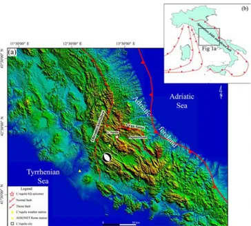
A Mw 6.3 earthquake struck the Abruzzo region in
cen-tral Italy on 6 April 2009 (01:32 UTC), and its epicenter was located at 42.34◦N, 13.38◦E (depth of 9.5 km), which is near the city of L’Aquila (Fig. 1). According to the Isti-tuto Nazionale di Geofisica e Vulcanologia (INGV), many strong foreshocks had been occurring since December 2008, and more than 10 000 aftershocks had been recorded until September 2010. Previous geological studies stated that the present-day geologic setting along the Italian peninsula re-lated to the N–S convergence zone between the African and the Eurasian plates is particularly complex because differ-ent processes occur simultaneously and in close proximity to one another (Montone et al., 2004; Galadini and Galli, 2000). Central Italy experiences active NE–SW extensional tectonics approximately perpendicular to the Apenninic fold and thrust belt (Montone et al., 2012); a city in this region is L’Aquila, which is bounded by the Olevano–Antrodoco and Gran Sasso thrusts at the west and north sides, respectively. In 2009, the L’Aquila mainshock occurred as a result of nor-mal faulting (Paganica fault, PF) and as a primary response to the Tyrrhenian basin opening faster than the compression between the Eurasian and African plates (USGS, 2009).
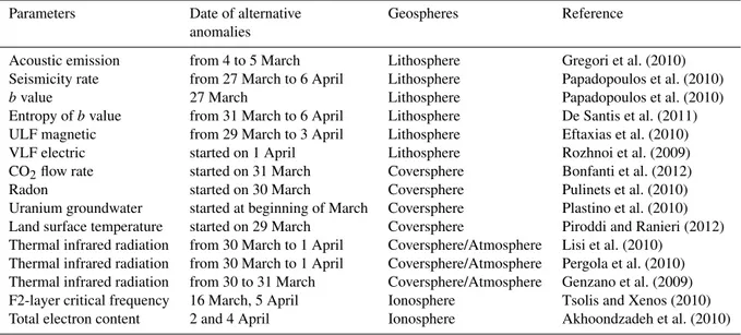
A large number of the precursory anomalies of the 2009 L’Aquila earthquake were reported after the main-shock. These anomalous parameters included thermal prop-erties, electric and magnetic fields, ionospheric parameters, underground water, gas emission, crust stress, and seismic-ity (Akhoondzadeh et al., 2010; Bonfanti et al., 2012; Cian-chini et al., 2012; De Santis et al., 2011; Eftaxias et al., 2009; Genzano et al., 2009; Gregori et al., 2010; Lisi et al., 2010; Papadopoulos et al., 2010; Pergola et al., 2010; Piroddi and Ranieri, 2012; Plastino et al., 2010; Pulinets et al., 2010;
Figure 1. Simplified tectonic and topographic map of central Italy. (a) Digital elevation model from the Shuttle Radar Topography Mis-sion (SRTM) data showing the epicenter of the 2009 L’Aquila earth-quake (white star) along with its focal mechanism solution (FMS). The FMS was obtained from the U.S. Geological Survey’s National Earthquake Information Center (Di Luccio et al., 2010; Piroddi et al., 2014). (b) The main thrusts in Italy, with the black solid line box showing the geographical location of (a) (Benoit et al., 2011).
Rozhnoi et al., 2009; Tsolis and Xenos, 2010). Many of the existing reports revealed the existence of temporal quasi-synchronism among the several anomalies of different pa-rameters related to different geospheres (Table 1). We be-lieve that the geosphere coupling effects could support or in-terpret the occurrence of the various precursory anomalies of the 2009 L’Aquila earthquake. Moreover, we hypothesize the possible role of the coversphere in the process of LCAC, in which the radiation transmission caused anomalous thermal infrared signals in satellite sensors.
Air ionization and ion hydration are generally known as critical physical processes that result in different types of earthquake precursors between the ground surface and the lower atmosphere (Pulinets and Ouzounov, 2011; Freund, 2011). However, a corresponding observation of complemen-tary parameters related to the coversphere, such as soil hu-midity, water vapor, heart flux, and atmospheric aerosol, is not comprehensive enough to obtain a plain validation.
The seismic b value describes the fundamental relation-ship between the frequency and the magnitude of earth-quakes, which is known as the Gutenberg–Richter law (Gutenberg and Richter, 1944), and is widely applied in tec-tonic seismicity studies. The b value represents the size dis-tribution of abundant seismic events of small to moderate magnitudes; it is associated with several physical properties, such as regional stress, material homogeneity, and tempera-ture gradient (Gulia and Wiemer, 2010; Mogi, 1962;
Schor-Table 1. Reported multiple-parameter anomalies associated with the Mw6.3 2009 L’Aquila earthquake.
Parameters Date of alternative Geospheres Reference anomalies
Acoustic emission from 4 to 5 March Lithosphere Gregori et al. (2010) Seismicity rate from 27 March to 6 April Lithosphere Papadopoulos et al. (2010) bvalue 27 March Lithosphere Papadopoulos et al. (2010) Entropy of b value from 31 March to 6 April Lithosphere De Santis et al. (2011) ULF magnetic from 29 March to 3 April Lithosphere Eftaxias et al. (2010) VLF electric started on 1 April Lithosphere Rozhnoi et al. (2009) CO2flow rate started on 31 March Coversphere Bonfanti et al. (2012)
Radon started on 30 March Coversphere Pulinets et al. (2010) Uranium groundwater started at beginning of March Coversphere Plastino et al. (2010) Land surface temperature started on 29 March Coversphere Piroddi and Ranieri (2012) Thermal infrared radiation from 30 March to 1 April Coversphere/Atmosphere Lisi et al. (2010)
Thermal infrared radiation from 30 March to 1 April Coversphere/Atmosphere Pergola et al. (2010) Thermal infrared radiation from 30 to 31 March Coversphere/Atmosphere Genzano et al. (2009) F2-layer critical frequency 16 March, 5 April Ionosphere Tsolis and Xenos (2010) Total electron content 2 and 4 April Ionosphere Akhoondzadeh et al. (2010)
lemmer et al., 2005; Schorlemmer and Wiemer, 2004, 2005; Tormann et al., 2015; Urbancic et al., 1992; Warren and Latham, 1970; Wiemer and Wyss, 2002; Wyss and Wiemer, 2000). Hence, the b value is possibly a proxy of crust stress conditions and could therefore act as a crude stress meter for seismicity observed in the lithosphere (Tormann et al., 2014). Although the time sequence of the b value based on microseismicity data before and after the 2009 L’Aquila earthquake has been analyzed and has revealed the quasi-synchronous features of the b value relative to other pa-rameters (De Santis et al., 2011), the correlations of var-ious anomalies in the coversphere and lithosphere remain unclear because of the absence of essential geospatial anal-ysis. Moreover, various factors directly influence the ther-mal radiation signals observed by satellite sensors; these factors include atmosphere properties (absorption, scatter-ing, and emission of water vapor, as well as aerosol par-ticles), thermal condition of the Earth’s surface (meteoro-logical condition, soil moisture and components, vegetation cover, and surface roughness), and the complex thermal pro-cess of geo-objects. In view of remote sensing physics and the LCAC effect, we have reason to believe that other pa-rameters characterized by the above-mentioned factors in re-lation to the coversphere and atmosphere should have pre-sented temporal quasi-synchronism and spatial consistency with the reported thermal anomalies before the mainshock of the 2009 L’Aquila earthquake.
Several hydrothermal parameters related to the cover-sphere and atmocover-sphere, including soil water and temperature, precipitable water, air temperature, and atmospheric aerosol, are comprehensively analyzed in this study to explore the possible LCAC effects preceding the 2009 Mw6.3 L’Aquila
earthquake. The 3-D dynamic evolution of the b value is also analyzed to further investigate the potential correlations of
multiple-parameter anomalies related to the coversphere and the dynamics of the lithosphere. Furthermore, the variation of some parameters after the mainshock is analyzed for compar-ison. From retrospective analyses of data collected prior to this earthquake, we finally attempt to discuss the geosphere coupling process and propose a model for interpreting the LCAC effects with the support of previous geophysical re-searches.
2 Analysis of hydrothermal parameters 2.1 Data and method
Four parameters related to the coversphere and atmo-sphere, namely, volumetric soil moisture level 1 (SML1) at 0–7 cm b.g.l. (below ground level), soil temperature level 1 (STL1) at 0–7 cm b.g.l., near-surface air tempera-ture at a height of 2 m (TMP2m), and precipitable water of the entire atmosphere column (PWATclm), were analyzed in long-term intervals and within 2 months before and after the mainshock. The six-hourly values of the SML1 and STL1 parameters were 00:00, 06:00, 12:00, and 18:00 UTC ev-ery day according to ERA-Interim reanalysis dataset, which is a series of the latest global atmosphere reanalysis prod-ucts produced by the European Centre for Medium-Range Weather Forecasts (ECMWF) to replace the 40. ERA-Interim covers the data-rich period since 1979 and con-tinues to present time. The gridded data were transformed into a regular N128 Gaussian grid (512 lines of longitude and 256 lines of latitude) with 0.71◦×0.71◦spatial resolu-tion (http://apps.ecmwf.int/datasets/data). The TMP2m and PWATclm datasets also comprised six-hourly values based on the Final (FNL) Operational Global Analysis system of the National Center for Environmental Prediction (NCEP),
which was produced with the same NCEP model as that used for the Global Forecast System (http://rda.ucar.edu/datasets). The NCEP-FNL data were also represented in a Gaussian grid with 1◦×1◦spatial resolution (360◦longitude by 180◦ latitude). All the data from March and April 2000–2009 were investigated. The datasets containing information on the air temperature and aerosol optical depth (AOD) from ground-based observations were considered and compared with the results from the assimilation data to verify the key coupling process of the anomalies. The air tempera-ture data were obtained from the L’Aquila weather station (42.22◦N, 13.21◦E; elevation of 680 m, shown as yellow cir-cle in Fig. 1), whereas the AOD data were obtained from the Rome station (41.84◦N, 12.65◦E; elevation of 130 m, shown as yellow triangle in Fig. 1) of the Aerosol Robotic Networks (AERONET, http://aeronet.gsfc.nasa.gov/). With respect to the epicenter, the Rome station, which uses the Cimel Elec-tronique CE318 sun photometer to measure aerosol optical properties, is the only nearby station with available data.
First, we analyzed the long time series of the SML1, STL1, TMP2m, and PWATclm data on the epicenter pixel (42.34◦N, 13.38◦E; shown as black rectangular boxes in Figs. 3–6). To compare the data in 2009 with historical data, the mean (µ) and standard deviation (σ ) were calculated using data from multiple years (2000–2008). Here a devi-ation with overquantity more than 1.5σ , being a threshold, was defined as a probable anomaly for each parameter on the epicenter pixel. For confutation analysis, we also com-pared the 2009 data with the data from 2006 (green line in Fig. 2), which is regarded as a silent year for its seismic-ity rate (≤ 10 earthquakes with M3+ according to the INGV catalog for this area). After processing the preliminary data and checking for errors, we found that the anomalies of mul-tiple parameters were more remarkable at 06:00 UTC than in other moments. Thus, all the ERA-Interim and NCEP-FNL data at 06:00 UTC were selected uniformly for informa-tion extracinforma-tion and anomaly recogniinforma-tion. The daily averages and the maximum and minimum values based on the data from the ground-based stations were analyzed subsequently. In addition, we used the 5th and 95th percentile box plots of AOD532 nm each day to effectively express the variations in
the daily averages and maximum and minimum values as a result of the differences in the daily data records (Che et al., 2014).
Second, the spatial distributions of the SML1, STL1, TMP2m, and PWATclm data were analyzed. Considering the complex influences and possible uncertainties with regard to seasons, terrain, weather, and latitude, we obtained the differ-ential images of the changed parameters (1P ) by subtracting the 2009 daily value from the means of multiple years. The result reflected the current deviation of the parameter value referring to a normal background, i.e.,
1Pt=Pt−µt=Pt− 1 n n X i=1 P_i, (1)
where Pt is the daily value of a parameter in 2009 and µt is
the corresponding daily mean estimated over the years 2000– 2008. The 1Pt images on the same day in 2006 were
ap-plied for comparison, and the Pifor 2006 was adjusted to the
means of 2000–2008, except 2006.
2.2 Spatiotemporal features of hydrothermal parameters
2.2.1 SML1, STL1, PWATclm, and TMP2m from assimilation datasets
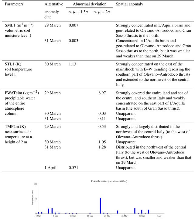
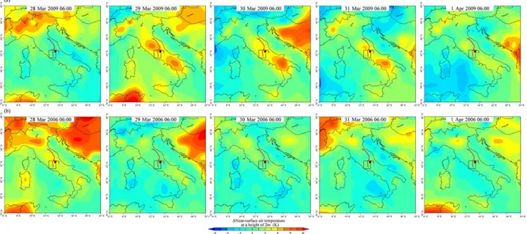
In the coversphere, the soil is an important layer for the trans-mission of mass and energy from the lithosphere to the at-mosphere. The hydrologic conditions and thermal proper-ties of surface soil could be disturbed in the seismogenic process. Our intuitive analysis showed that the variation curve of the SML1 parameter of the epicenter pixel ap-peared to decrease from March to April in 2009 and 2006 (Fig. 2a). However, five anomalies exceeded µ + 1.5σ before the 2009 L’Aquila mainshock, with the maximum anomaly occurring on 5 March. In the context of the gradual seasonal increase of STL1, its anomalous variation became obvious on 30 March, with the value being the maximum for that month (Fig. 2b). Although the variation amplitudes of SML1 on 29 and 31 March were less than those of the former two peaks, these dates were quasi-synchronous with STL1 (Fig. 2b). Hence, the water content and temperature in the surface soil significantly changed at the end of March 2009. Comparing the PWATclm behavior in 2009 with its relatively stable fluctuation in 2006, which acts as the normal back-ground, the PWATclm parameter exhibited evident peaks on 29–31 March; the highest value reached 27.8 kg m−2, which significantly exceeded µ + 2σ (Fig. 2c). PWATclm repre-sents the total water vapor content of the atmosphere col-umn; in this work, this parameter indicated that the mois-ture budgets on the surface and atmosphere layer were dis-turbed by something abnormal. Air temperature is a di-rect parameter related to the thermal variation in the cov-ersphere. We also found continuous anomalous peaks of TMP2m from 29 March to 1 April 2009. The values in this time window exceeded µ + 2σ , except on 1 April (Fig. 2d). Considering the reported anomalies in Table 1, we propose that the quasi-synchronous period characterized by multiple-parameter anomalies preceding the L’Aquila earthquake is likely the time window from 29 March to 1 April 2009. The details of the abnormal deviation of the parameters during this time window are shown in Table 2.
We mapped the image series of each 1Pt as the
differ-ence between the daily value and the historical mean (µ) to investigate the spatiotemporal evolution of the investi-gated parameters. Figure 3a shows that the area with an
ab-Figure 2. Time series of four hydrothermal parameters: volumetric soil moisture level 1 (a), soil temperature level 1 (b), precipitable water of the entire atmosphere column (c), and near-surface air temperature at a height of 2 m (d), on the epicenter pixel from March to April 2009, and its comparison with historical data over the same period. The red and orange lines show the value of (µ + 2σ ) and (µ + 1.5σ ), respectively; the green and black lines show the value in 2006 (as a normal background) and 2009, respectively.
normal increment of 1SML1 was located in the L’Aquila basin on 29 and 31 March 2009 and that the local 1SML1 reached 19.5 to 21 K in the epicenter grid. By contrast, the spatial pattern in 2006 was characterized as normal with clear homogeneity for the land in central Italy (Fig. 3b).
This result implied that the moisture on the upper surface soil layer of the seismogenic zone abruptly increased before the mainshock. Although significantly anomalous 1SML1 occurred in northern Italy, such an anomaly was attributed to regional weather conditions and to be unrelated to the
Figure 3. Spatial distributions of deviated volumetric soil moisture level 1 (1SML1) at 06:00 UTC from 28 March to 1 April 2009 (a) and 2006 (b), respectively. The black spot indicates the epicenter of the mainshock, the black rectangular box indicates the epicenter pixel, and the red line indicates the related main fault system.
Figure 4. Spatial distributions of deviated soil temperature level 1 (1STL1) at 06:00 UTC from 28 March to 1 April 2009 (a) and 2006 (b), respectively. The black spot indicates the epicenter of the mainshock, the black rectangular box indicates the epicenter pixel, and the red line indicates the related main fault system.
L’Aquila earthquake because of its large area and remote distance. Different from that of 1SML1, the spatial anoma-lous field of 1STL1 initiated on 29 March and appeared distinguishably northwest of the epicenter of the mainshock on 30 March 2009 (Fig. 4a), especially along the southern segment of the Olevano–Antrodoco thrust (Fig. 1). This ab-normal pattern did not appear in 2006 (Fig. 4b). According
to the local meteorological data (Fig. 5), the particular spa-tiotemporal evolution of 1SML1 and 1STL1 did not result from precipitation. As changes in soil water stimulate ther-mal change, a short delay in the change in soil temperature relative to soil moisture is possible. In this work, we revealed a 1-day delay between the increases in soil temperature and soil moisture.
Table 2. Hydrothermal parameter anomalies from 29 March to 1 April 2009 (quasi-synchronous period). Parameters Alternative Abnormal deviation Spatial anomaly
anomaly > µ +1.5σ > µ +2σ date
SML1 (m3m−3) 29 March 0.007 Strongly concentrated in L’Aquila basin and volumetric soil geo-related to Olevano–Antrodoco and Gran moisture level 1 Sasso thrusts to the north.
31 March 0.003 Concentrated in L’Aquila basin and geo-related to Olevano–Antrodoco and Gran Sasso thrusts to the north, but it was smaller and weaker than that on 29 March. STL1 (K) 30 March 1.13 Strongly concentrated on the east of the soil temperature mainshock with E–W trending (crossing the level 1 southern part of Olevano–Antrodoco thrust) and extended to the northwest of the central Italy.
PWATclm (kg m−2) 29 March 8.97 Strongly covered the entire land and sea of precipitable water the central and southern Italy and weakly of the entire concentrated on the east part of L’Aquila atmosphere basin (the south of Gran Sasso thrust). column 30 March 0.03 Unapparent
31 March 0.11 Unapparent
TMP2m (K) 29 March 0.53 Strongly and largely distributed in the near-surface air northwest of the central Italy (to the west of temperature at a Olevano–Antrodoco thrust).
height of 2 m 30 March 1.05 Unapparent
31 March 1.28 Distributed in the northwest of the central Italy (to the west of Olevano–Antrodoco thrust), but was smaller and weaker than that on 29 March.
1 April 0.571 Unapparent
Figure 5. Daily precipitation at L’Aquila station from 1 March to 5 April 2009.
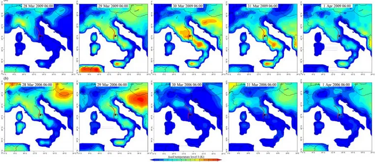
In the case of an abnormal variation in temperature and moisture in the surface soil layer, hydrothermal conversion becomes increasingly significant on the surface and in the at-mosphere because of the wide, open space. Compared with PWATclm in almost all the Italian territories and surround-ing seas dursurround-ing the silent period, 1PWATclm showed a sud-den increase on 29 March 2009; it then quickly dropped to a relatively normal level on 31 March, similar to the case in 2006 (Fig. 6). Although the abnormal area of 1PWATclm covered the entire Italy, a weaker abnormal area appeared
in the L’Aquila basin on 29–31 March and extended to the southeast (Fig. 6a), where it equaled 1SML1 on 29– 31 March (Fig. 4a). We considered the possibility of the re-gional anomalous signal related to the seismogenic process being masked by an intensive air–sea interaction in a large area on those days. Obviously, both the spatial anomalies of 1SML1 and 1PWATclm were not controlled by topo-graphic conditions. Particularly, the normal spatial pattern of 1TMP2m in central Italy on 28 March to 1 April 2006 was slightly higher than that over the sea and notably lower than
Figure 6. Spatial distributions of deviated precipitable water of the entire atmosphere column (1PWATclm) at 06:00 UTC from 28 March to 1 April 2009 (a) and 2006 (b), respectively. The black spot indicates the epicenter of the mainshock, the black rectangular box indicates the epicenter pixel, and the red line indicates the related main fault system.
Figure 7. Spatial distribution of deviated near-surface air temperature at a height of 2 m (1TMP2m) at 06:00 UTC from 28 March to 1 April 2009 (a) and 2006 (b), respectively. The black spot indicates the epicenter of the mainshock, the black rectangular box indicates the epicenter pixel, and the red line indicates the related main fault system.
that at the northern border of the Italian territory (Fig. 7b). However, an anomalous spatial distribution of 1TMP2m oc-curred on 28 and 30 March 2009, mainly in the intermoun-tain area northwest of the mainshock epicenter (Fig. 7a). The anomalies of the four investigated parameters were dis-tributed mainly in the L’Aquila basin or in the
intermoun-tain area to the northeast of the mainshock epicenter on 29–31 March. Thus, we inferred that the regional topog-raphy (Apennine range and L’Aquila basin) and tectonics (Olevano–Antrodoco and Gran Sasso thrusts) in central Italy could have induced the spatial correlations of these anoma-lies.
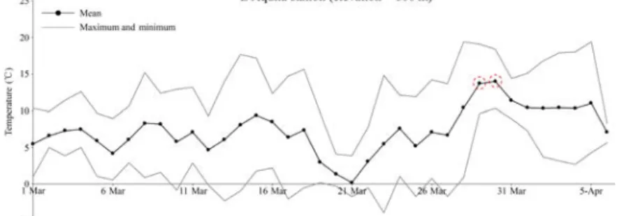
Figure 8. Daily average and maximum and minimum values of air temperature at the L’Aquila station from 1 March to 5 April 2009.
Figure 9. Time series of AOD at the Rome station of AERONET from 3 March to 6 April 2009. (a) AOD at 440, 532, and 675 nm; (b) daily average and maximum and minimum values of AOD532 nm, as well as the 5th and 95th percentile box plots.
2.2.2 Air temperature and AOD from ground-based stations
To investigate possible thermal fluctuations in situ and to sup-port the potential coupling effects of such fluctuations on the ground surface, we collected air temperature and AOD data from ground-based stations. Figure 8 shows that both the daily averages and the maximum and minimum values of air temperature at the L’Aquila weather station reached their peaks on 29 and 30 March 2009 (Fig. 8). Figure 9 shows the AOD variations had fluctuated in three time windows with the abrupt AOD increase on 16 March, 30 March, and 3– 6 April 2009, respectively. The dates in which the anomalous values of air temperature and AOD were observed were con-sistent with those for SML1, STL1, PWATclm, and TMP2m. In particular, the general AOD values were less than 0.3 (Fig. 9a); however, the maximum AOD532 nm reached 0.37,
0.3, and 0.46 in the three time windows, whereas the rest of the AOD532 nm varied around 0.07–0.26, which is the same
as those on clear days (Fig. 9b). Although the Rome station
of AERONET is far from the epicenter and the increase in AOD was weak, the observed AOD data somehow served as the reference value for L’Aquila. The secondary organic aerosol (SOA) in the atmosphere is generated from the pho-tochemical reaction of gas phase precursors, such as sul-fur (SO2) and nitrogen (NO2) volatiles, as well as ozone (O3)
(Janson et al., 2001; Rickard et al., 2010), whereas the photo-chemical production of O3is a result of the photo-oxidation
of methane (CH4) and carbon monoxide (CO) (Dentener et
al., 2006; Crutzen, 1974). The increased CH4degassing soon
after the L’Aquila earthquake (Voltattorni et al., 2012; Quat-trocchi et al., 2011) could be hints of O3precursors. Hence,
the anomalous increments of aerosol might have been caused by the formation of SOA particulates as a result of the photo-chemical production of O3from degassed CH4. In addition,
the low precipitation in March 2009 (Fig. 5) indicated that the weather condition during this period was acceptable and that the anomalous PWATclm increment in the epicenter pixel on 29 March 2009 was not caused by rainfall.
2.3 Summary of the hydrothermal parameter analysis The following seismic anomalies were determined to be pos-sible according to the quasi-synchronism analysis of the ab-normal changes of six hydrologic and thermal parameters re-lated to the coversphere and atmosphere and according to the spatial evolution analysis of the images of the changed val-ues. (1) The anomalies were observed mainly in the L’Aquila basin to the southeast of the mainshock epicenter (1SML1 and 1PWATclm) or in the Apennines range northwest of the mainshock epicenter (1STL1 and 1TMP2m). (2) The spatial migration of the hydrologic and thermal changes in the upper surface soil layer (1SML1 and 1STL1) could have indicated the reformation and redistribution of mass and energy transmitted from the lithosphere to the coversphere. (3) The spatial distribution of the increased air temperature near the surface was consistent with that of the soil tem-perature. Hence, the thermal transmission process was sta-ble from the coversphere to the atmosphere and was con-trolled by regional tectonics in central Italy. (4) Although the improvement in the precipitable water content in the atmo-sphere on 29 March 2009 was masked by its high values in the surrounding large area, the anomalous weak values in the L’Aquila basin suggested something particularly related with the seismogenic zone, such as the water in gaseous or liquid state was influenced by local soil structure (aquifers) and sur-face topography. Considering these findings, we propose that the anomalies be interpreted as the geosphere coupling ef-fects preceding the 2009 L’Aquila earthquake.
3 Seismic b value 3.1 Data and method
The earthquake catalog for computing the b value in this work was obtained from INGV (ISIDE: http://iside.rm.ingv. it). This catalog covers all of Italy and its surrounding re-gions. We analyzed the seismic data covering the periods from 16 April 2005 to 19 December 2012, during which 94 953 events were recorded. Considering data quality and tectonic regimes related to the 2009 L’Aquila earthquake, we excluded in the analysis the events that occurred at a depth of over 40 km and limited the study area to the region within the 80 km radius of the epicenter of the L’Aquila mainshock. Referring to the changes in the slope of the plot of the cu-mulative number of events, we identified three-staged phases of different recording qualities, with P1-1 and P1-2 denoting the conditions before the 2009 L’Aquila earthquake and P2 denoting the conditions after the 2009 L’Aquila earthquake. The details are as follows:
– Phase P1-1: 3552 events from 18 April 2005 to 15 Au-gust 2007;
– Phase P1-2: 2742 events from 16 August 2007 to 5 April 2009;
– Phase P2: 19 782 events from 6 April 2009 to 30 November 2009.
In seismology, the classical Gutenberg–Richter law (Guten-berg and Richter, 1944) is introduced as follows:
log N (M) = a − bM, (2)
where N is the number of earthquakes with magnitudes greater than or equal to M in a given region and in a time interval; a and b are constants that describe the productivity and relative size distribution of the area of concern, respec-tively. The study of the b value has been widely performed (Mogi, 1962; Urbancic et al., 1992; Warren and Latham, 1970), and its variations have been found to be caused by re-gional stress, rock properties, and temperature gradient. Us-ing the software package ZMAP (Wiemer, 2001), we com-puted the maximum-likelihood b values with the following Eq. (3):
b = log e M − Mo+1M2
, (3)
where M is the mean magnitude and Mois the minimal
mag-nitude of the given samples; 1M is the uncertainty in magni-tude estimation and is usually set to 0.1. The sample was con-sidered complete down to the minimal magnitude Mc≤Mo,
which also referred to as the magnitude of completeness (Mc,
Schorlemmer and Wiemer, 2004).
To detect the dynamic features of the b values, we esti-mated the b values with Eq. (3) in moving (partly overlap-ping) time windows. Generally, the sampling window con-tains 200 seismic events, 10 % of which comprise the slid-ing/overlapping window (i.e., 20 events), and the b value ac-tually is estimated from part samples before and after each time node. To visualize the spatial distribution of the b val-ues, all events in the study area were projected onto a coor-dinate plane with a gridded space of 0.1◦longitude by 0.1◦ latitude. At each grid node, we sampled all the events within a radius of 20 km and determined their b values if at least Nmin=30 events were available. Following the work of De
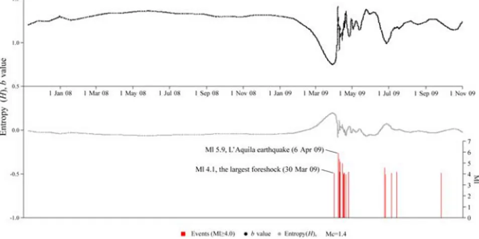
Santis et al. (2011), we also calculated the corresponding Shannon entropy of the earthquake related to the b value, i.e.,
H (t ) = k −log b(t ) (k ≈ 0.072). (4) This entropic quantity allows the measurement of the level of disorder of the seismic system and the missing informa-tion or uncertainty because it is universally considered a fun-damental macroscopic physical quantity that describes the properties of complex geosystemic evolutions, such as that of the seismogenic system in the lithosphere (De Santis et al., 2011).
3.2 Spatiotemporal features
To compare the results of De Santis et al. (2011), we also reduced the catalog by Mc=1.4 for the time series analysis
Figure 10. Time series of b value (above plot), Shannon entropy (H ; intermediate plot), and seismic events (Ml ≥ 4.0; bottom plot) during phases P1-2 and P2.
of the b values from phase P1-2 to phase P2. Following the preceding stable phase P1-1 and the fore part of P1-2 before the January in 2008, the b value drastically decreased as the mainshock approached. Figure 10 shows that the curve drops to the lowest point of b = 0.747 about 27 March 2009, i.e., ∼10 days before the mainshock or a few days before the oc-currence of various thermal anomalies (Piroddi and Ranieri, 2012; Piroddi et al., 2014). Meanwhile, the entropy gradu-ally increased to reach the peak (almost 0.2, Fig. 10) dur-ing the same period after a long (almost) stable period and then dropped 1 week before the mainshock. Note that the exact time when the peaks were reached (minimal b value and maximal entropy) could not be detected properly be-cause ZMAP applies a moving sliding window containing 200 events for computation. Hence, each curve was slightly affected by what was preceding and what was following the given moment of estimation. Moreover, the b value (or the entropy) appeared to have moved rapidly to the minimum (or the maximum) on the day of the mainshock. This con-dition indicated that the regional stress was rapidly released and that faults ruptured quickly close to the mainshock. Both the b value and entropy were unstable after the mainshock because of the aftershocks. Although we used a moving win-dow with ZMAP to calculate the b value, and, in turn, the entropy, the minimum value of b value and the maximum value of the entropy just around the time of the mainshock is real and not an artefact. Figure 11 shows a smaller inter-val of time where the entropy has been estimated in subse-quent non-overlapping intervals of 30 seismic events each: it is clear from the observed estimates (triangles) that the begin-ning of the increase of the entropy was well before the main-shock (when the entropy exceeds two times the standard de-viation, sigma, estimated over the whole interval), with max-imum at around the moment of it (when the entropy exceeds even 10 times the standard deviation). For a better visual-ization of the observed general behavior of the entropy, we also draw the gray curve that defines a reasonable smoothing
Figure 11. Shannon entropy for L’Aquila seismic sequence from around 1.5 year before the mainshock to around 1 year after, calcu-lated for a circular area of 80 km around the mainshock epicenter. The gray curve defines a reasonable smoothing of the entropy val-ues: 15-point FFT before the mainshock and 50-point FFT smooth-ing after the mainshock. Sigma is the standard deviation estimated over the whole interval (w.r.t means with respect to).
of the entropy values: 15-point FFT (fast Fourier transform) before the mainshock and 50-point FFT smoothing after the mainshock. The different kind of smoothing is related to the different rate of seismicity before and after the mainshock.
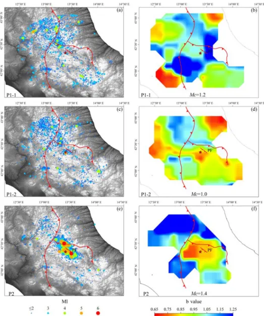
Then we split the catalog into two subsets in terms of their magnitudes, which were lower than the estimated complete-ness values, i.e., Mc=1.2 and Mc=1.0. The spatial
distri-butions of the b values clearly differed in the two phases be-fore the L’Aquila earthquake (Fig. 12b and d). In phase P1-1, the b values in the L’Aquila basin and its surroundings were about 1.0, which indicated a normal regional stress level because b = 1.0 is a universal constant for earthquakes in general (Schorlemmer et al., 2005; Kagan, 1999). The
Figure 12. Spatial distributions of epicenters (a, c, e) and b value (b, d, f) before and after the mainshock of the L’Aquila earthquake at three-staged phases (the red star and the red lines represent the mainshock and main fault system, respectively).
areas of high b values (b ≥ 1.2) were located in the south and east of the impending L’Aquila hypocenter, which in-dicates less seismicity in these areas. By contrast, some far external areas with low b values were not relevant to the seismic sequence because of existing rare seismic events in these areas (Fig. 12a). However, most of the relatively high b values in phase P1-1 changed to extremely low b values (b ≤ 0.8) in phase P1-2. In particular, a relatively homoge-neous strip of low b values extended westward from the im-pending hypocenter and crossed the southern segment of the Olevano–Antrodoco thrust. This effect indicated the devel-opment of rock mass fracturing, i.e., seismicity, in the east-to-west direction, especially in the south of the impending hypocenter. Coincidentally, this strip representing a fractured area was consistent with the location of the strongest varia-tion in soil temperature on 30 March (Fig. 4a). Most of the
other parts along the Olevano–Antrodoco and Gran Sasso thrusts retained relatively low seismicity. The changed spa-tial patterns of the b values from P1-1 to P1-2 indicated more and more rock fractures and energy releases were develop-ing in the seismogenic zone before the L’Aquila earthquake. These conditions clearly reflected the intensive seismicity and significantly rapid accumulation of rock fractures occur-ring near the approaching L’Aquila mainshock hypocenter relative to other places. Figure 12f shows the spatial distribu-tion of the b values after the L’Aquila earthquake. Different from what happened before the mainshock, the low b values occurred in the L’Aquila basin and its surroundings because of the Paganica fault rupture and the subsequent aftershocks (Fig. 12e). We also notice that the extremely low b values (red and orange area) covered the entire Gran Sasso thrust and the footwall of the Olevano–Antrodoco thrust. This
ob-servation indicated that the developed cracks and ruptured rocks, which resulted from the normal faulting of the Pa-ganica fault, passed through the entire Gran Sasso thrust but stopped at the footwall of the Olevano–Antrodoco thrust.
We also selected the geological section (section 1 in Fig. 13a) used by Piroddi et al. (2014) to show the variations in the b values with depth before the L’Aquila earthquake. Another section of equal length (section 2 in Fig. 13a), which was perpendicular to section 1 crossing the epicenter, was analyzed to identify further the differences in the stress dis-tribution and rock failure between section 1 and 2. Events above depth = 20 km were sampled to calculate the b values in a buffer of 20 km from the two section lines (Fig. 13a). In Fig. 13b, the spatial distribution of the low b value ap-peared around the hypocenter and extended about 25 km to SWW of the hanging wall of the Paganica fault along sec-tion 1. This distribusec-tion illustrated the stress accumulasec-tion at a depth of 10 km, which is shown as an orange low-b-value stripe in Fig. 12d. A relatively low b low-b-value zone was also observed between the Paganica fault and the Gran Sasso thrust. In addition to the area of the impending hypocenter, the spatial image of the b value along section 2 confirmed that the low b value zone was near the Gran Sasso thrust and about 20 km from NNW of the Olevano–Antrodoco thrust (Fig. 13). According to this result, the geo-zones of stress concentration and rock failure were related not only to the normal seismogenic fault (Paganica fault) but also to the two large thrusts (Olevano–Antrodoco and Gran Sasso thrusts) long before the L’Aquila earthquake. The lowest b values centered on the hanging wall of the Paganica fault at depths of 5–15 km (Fig. 13b and c). As shown in the vertical imag-ing section, the low b values partly connected the Paganica fault to the Gran Sasso thrust.
Moreover, the relations between the b values and the geo-logical depth in the whole study area were mapped to inves-tigate the change in the stress environment of the deep earth at different phases (Fig. 14). We observed a similar varia-tion trend of the b values spatially related to depth before (phase P1-2) and after (phase P2) the mainshock. The general bvalue curves at both phases initially increased from 20 km to about 12.5 km, rapidly dropped to the minimum at 9.5 km, and finally increased to high values at 5 km, which is the low-est depth indicated in the hypocenter records. Hence, the re-gional crust stress accumulated at a depth of about 9.5 km, whereas the stress dropped at the deep and low crusts. The stress change was stable at a depth of more than 20 km in the study area. Obvious curve reversals appeared twice at depths of 8–12.5 km before the mainshock (Fig. 14a). Hence, het-erogeneous lithostratigraphic properties affected rock fail-ure and led to different stress states in the study area. Ac-cording to CROP 11 (“CROsta Profonda,” literally “Deep Crust”) studies on the near-vertical seismic reflection profiles crossing central Italy, which were supported by the CROP Project and were initiated in the mid-1980s with joint fund-ing from the National Research Council, AGIP Oil Company,
and ENEL (National Electric Company) (Di Luzio et al., 2009; Patacca et al., 2008; Tozer et al., 2002), the anomalous curve reversals resulted from the lithostratigraphic difference among the Mesozoic Gran Sasso–Genzana unit, Queglia unit, Morrone–Porrara unit, and even the western Marsica– Meta unit. These carbonate units mainly contain shallow-platform dolomite and limestone, which were overlaid dis-conformably by Miocene carbonate deposits and siliciclastic flysch deposits. In addition, the Queglia unit and the deeper Maiella unit contain Messinian evaporite and marl. Thus, the anomalous reversal of the b value with depth could be the re-sult of the unconformable Mesozoic–Cenozoic contact; the mixed flysch, evaporate, and marl might have also affected the counter-regulation of stress accumulation. Hence, we in-fer that 10 ± 5 km was the main depth range of the seismic stress variation associated with the L’Aquila earthquake. 3.3 Summary of the seismic analysis
The time series analysis of the b values in phases P1-2 and P2 shows that, after late December 2008, the b value (or the entropy) rapidly went to the minimum (or the maximum), specifically on 27 March 2009 (10 days before the main-shock), and then wildly fluctuated closely before and af-ter the mainshock. The date of occurrence of the anoma-lously low b value coincided with that of the reported thermal anomalies, which indicated the rapid release of crust stress and fracturing of rock mass and/or faults. Compared with that in phase P1-1, the image of the b value in the latter phase P1-2 showed abnormally low b values near the im-pending L’Aquila hypocenter, as well as a homogeneous strip of low b values extending toward the east-to-east di-rection and crossing the southern segment of the Olevano– Antrodoco thrust. After the mainshock, the anomalous zone of low b values emerged in the L’Aquila basin and its sur-roundings because of rupturing and subsequent aftershocks. The 3-D spatial variation of the b value showed that the zone of low b values obviously appeared around the hanging wall of the Paganica fault at a depth of 5–15 km and extended to 20 km SWW. Similar anomalies of low b values closely related to two large thrusts were also observed in NNW of the impending hypocenter. In particular, anomalous reversals of the b values occurred twice at a depth of 8–12.5 km be-fore the mainshock, thus implying that unstable stress state did relate to heterogeneous lithostratigraphic properties. The revealed 3-D spatial pattern of the b values indicated that the space evolution characteristics of the stress accumulation prior to and immediately after the L’Aquila earthquake re-flect the spatial correlations among the L’Aquila earthquake and seismic faults in the central Apennines.
Figure 13. Spatial distribution of epicenters/hypocenters and b values from P1-1 to P1-2. (a) The outcrops of seismic faults and thrust, as well as all the epicenters of the foreshocks and the mainshock; (b) b values along section 1 crossing the mainshock epicenter and seismic faults and thrust (the black dots represent hypocenters); (c) b values along section 2 crossing the mainshock epicenter and seismic faults and thrust (the black dots represent hypocenters). OAt: Olevano–Antrodoco thrust, GSt: Gran Sasso thrust, Pf: Paganica fault.
Figure 14. The relation between the b values and hypocenter depths in phase P1-2 (a) and phase P2 (b). The dots indicate the average bvalues related to depth, the horizontal bars indicate the uncertainty in the b values, and the vertical bars indicate the depth range of the sampled hypocenters.
4 Discussions
As mentioned above, SML1, STL1, TMP2m, PWATclm, b value, and even AOD have quasi-synchronous time win-dow of anomalies. Obviously, this characteristic is not a sim-ple coincidence in time, and these anomalies are part of the general process of the development of the latest stage of the seismic cycle as well as the interaction of the complex open systems (Pulinets, 2011). Referring to the propagation of observed anomalies from ground up to the ionosphere, Pulinets et al. (2015) presented a physical background of ionization-induced geophysical processes in the lithosphere– atmosphere–ionosphere–magnetosphere system. However, the geophysical mechanism of the observed anomalies, es-pecially those related to the coversphere, necessitates further survey. Here, we attempt to provide a possible explanation of geophysical mechanism of the anomalies before L’Aquila earthquake in view of LCAC of the complex geo-systems. 4.1 Lithosphere: deep fluid and stress
The central Apennines are affected by a NE–SW-striking extension and uplift. This extension was responsible for the formation of intra-mountain basins, i.e., L’Aquila basin, bounded by the Gran Sasso and Mt. d’Ocre ranges. During the L’Aquila seismic sequence, the seismic events were fo-cused on the upper parts of the crust with a depth < 15 km; three main faults were activated by dip-slip movements in response to the NE–SW extension (Di Luccio et al., 2010). The ultimate cause of an earthquake is undoubtedly the crust stress exceeding the elastic limits of faults or rock mass. Crust stress is indeed affected by particular geo-environmental conditions, including faults, cracks, rock, and fluids, inside the lithosphere. Some studies based on the mea-surements of the ratio of compressional velocity to shear velocity and of seismic anisotropy have provided evidence that high-pressure fluid contributed to the rupturing of the 2009 L’Aquila earthquake (Di Luccio et al., 2010; Terakawa et al., 2010; Lucente et al., 2010). The contribution of flu-ids to the L’Aquila seismic sequence evolution was indepen-dently confirmed by Cianchini et al. (2012) through mag-netic measurements from the L’Aquila geomagmag-netic obser-vatory. As a result of the eastward migration of the compres-sive front since the early Miocene, the back-arc extension af-fected the Apennines chain, which was previously controlled by compressive tectonics (Di Luccio et al., 2010). Normal faults formed the L’Aquila basin and affected the Apennines chain in the Pleistocene period (Doglioni, 1995); moreover, several works have increasingly implicated fluids and their movement in the generation of the L’Aquila earthquake (Di Luccio et al., 2010; Terakawa et al., 2010; Lucente et al., 2010). Both the eastward compressive and NE–SW exten-sive stresses could have contributed to the deep fluid mi-gration to the potential epicenter area. Subsequently, seis-mogenic faults became weak as a result of the high
pres-sure of pore fluid and consequently reduced the stress level needed to break the rocks (Hubbert and Rubey, 1959). In particular, a proposed scenario suggested that the Paganica fault plane initially acted as a barrier to fluid flow (Lucente et al., 2010); hence, the fluid pressures at both sides of the fault were unbalanced. The foreshock sequence, especially the Ml 4.0 foreshock on 30 March, broke the barrier, thereby allowing fluids to migrate from north to south across the fault and change the Vp/ Vs ratios (Lucente et al., 2010). The
mi-grating fluids would have dilated the rock mass of the hang-ing wall and facilitated fault movement, leadhang-ing to earth-quake nucleation. The images of the b values in phase P1-2 (Fig. 12d) and along the two orthogonal sections (Fig. 13) clearly show the spatial distribution of rock failure develop-ment around the impending hypocenter and the large thrust at a depth of 10 ± 5 km in the crust, which correspond to fluid migration and high pore pressure, respectively.
At this point, we clarify basic issues on fluids. First, we discuss the composition of fluids and their sources. The Apennines located at the plate boundary are characterized by high heat flow and large-scale vertical expulsion, volcanoes, gas vents, mud pools, geysers, and thermal springs, which are typical surface features of fluid expulsion (Chiodini et al., 2004, 2011; Minissale, 2004). Two of the largest aquifers covering the Abruzzo region are the Velino and Gran Sasso aquifers (Fig. 15b), which consist of Meso-Cenozoic car-bonate formations (limestone and dolomite) of the Latium– Abruzzo platform and of platform-to-basin transitional do-mains (Chiodini et al., 2011). For the fluid solution, the rich groundwater breeds an ideal geo-zone for gas–water–rock re-actions. Fluids with CO2-rich gases are known to be involved
in the earthquake preparation process (Di Luccio et al., 2010; Terakawa et al., 2010; Lucente et al., 2010; Chiodini et al., 2011). Both the numerous CO2-rich gas emissions mainly
from the Tyrrhenian region and the large amounts of deeply derived CO2 dissolved by the groundwater of the aquifers
of the Apennines have been supported by geochemical and isotopic data (Chiodini et al., 2000, 2004, 2011; Minissale, 2004). The melting of the crust sediments of the subducted Adriatic–Ionian slab is a regional CO2source, and the
subse-quent upwelling of the mantle and the carbonate-rich melts would have induced the massive degassing of CO2 on the
Earth’s surface (Frezzotti et al., 2009). Thus, we conclude that the large quantities of CO2gas in the two aquifers not
only comprise a large portion of the dissolved inorganic car-bon derived from the Tyrrhenian mantle wedge and/or Adri-atic subducted slab in the deep Earth, but they also involve the progressive decarbonation of minerals of the carbonate formations in the shallow crust.
Second, we explain how fluids migrate. On the one hand, Chiodini et al. (2011) compared the geochemical composi-tion of Abruzzo gas of 40 large gas emission sites located in central Italy and found that the former becomes progres-sively rich in radiogenic elements (4He and 40Ar) and N2
Figure 15. An integrated representation of the geographical (coversphere) and geological (lithosphere) environments associated with the 2009 L’Aquila earthquake. (a) Zones of NTG anomalies from LST (land surface temperature) data overlapped by land covers (Piroddi and Ranieri, 2012); (b) the spatial distribution of tectonic faults, geological rocks, hydrogeological aquifers, and groundwater flows in the epicenter area and its surroundings (Chiodini et al., 2011).
in the east, thereby indicating the increasing residence time of the gas in the crust moving from west to east. On the other hand, Minissale (2004) performed a systematic analy-sis of published geochemical and isotopic data (together with new data) from the Apennines, including thermal and cold springs, gas vents (mostly CO2), and active and fossil
traver-tine deposits, and found that meteoric water precipitating in the high eastern Apennine ranges mixes with ascending east-ward magmatic, metamorphic, and geothermal fluids in the highly permeable Mesozoic limestone.
4.2 From lithosphere to coversphere: Earth degassing Before the mainshock, CO2-rich gases from different sources
would have been injected into the regional groundwater sys-tem (i.e., Velino and Gran Sasso aquifers) and moved up to the surface. Hence, the influx of CO2-rich gases can increase
pore pressure and flow rate. During the foreshock sequence, the development of fractures and cracks of rock mass would have facilitated the flow of fluids outside the aquifers in the shallow crust, which is bordered by the Olevano–Antrodoco and Gran Sasso thrusts. Meanwhile, electronic charge carri-ers of crustal rocks in the form of peroxy defects known as P-holes (Freund, 2011) could have been activated when the rock was stressed. Overpressured fluid could further reduce the friction of fault planes and reactivate faults. As a result of the widespread aquifers and the high permeability of car-bonate formations, underground fluids with CO2-rich gases
easily migrated upward to the coversphere under the acceler-ated stress condition. The rising of shallow underground fluid alters soil physical properties (i.e., soil moisture and temper-ature) and thereby affects different components of surface energy balance. A gas geochemical monitoring conducted in a natural vent close to the L’Aquila basin observed anoma-lous CO2gas flow variations in March and April 2009
(Bon-fanti et al., 2012). The intensive CO2degassing from ground
measurements confirms the emission of deeply originating gaseous fluids to the coversphere. The increase in greenhouse gas emission (i.e., CO2)is also an important mechanism of
pre-earthquake thermal anomalies. In addition, as radon gas might cause air ionization and variations in humidity and latent heat exchange, the anomalous Rn emanation before
the L’Aquila earthquake was recorded (Pulinets et al., 2010). Soil gas surveys (Voltattorni et al., 2012; Quattrocchi et al., 2011) revealed CO2and certain amounts of CH4and Rn as
released gas phases. Hence, we propose that the degassing of CO2, even CH4 and Rn, from the lithosphere to the
cover-sphere before the mainshock could have resulted in the com-plex lithosphere–coversphere coupling effect, which finally increased surface soil temperature and near-surface air tem-perature, and generated heavy TIR emissions.
4.3 From coversphere to atmosphere: air ionization As a transition layer from the lithosphere to the atmosphere, the coversphere affects the flow and exchanges of mass and
energy from the deep crust to the surface and atmosphere. As revealed by the ESA global land cover data produced from the Medium Resolution Imaging Spectrometer sensor aboard the Envisat satellite, the thermal anomalous zone based on the night thermal gradient (NTG) algorithm (Fig. 15a) was mainly covered by high vegetation, i.e., broadleaved decidu-ous forest, with strong water retention and developed root traits. Generally, high vegetation coverage represents high moisture in deep soil and improves the active characteris-tics of surface soil, including organic matter contents, which promote fluid concentration and movement through prefer-ential flow and root absorption (Chai et al., 2008; Millikin and Bledsoe, 1999). Hence, we propose that high vegeta-tion in central Italy facilitated the upward migravegeta-tion of CO2
-rich fluids inside the coversphere before the 2009 L’Aquila earthquake. We also suggest that this upward migration of CO2-rich fluids generated heavy thermal radiations because
of surface temperature rise from possible greenhouse effects together with latent heat release stimulated by the decay of radon and/or the activation of P-holes.
Air ionization is a fundamental factor of energy balance in the lower atmosphere. When underground gases are released on the surface, the air composition of the lower atmosphere must change. The leaked CO2and CH4gases on the surface
can serve as radon carriers, and α-particles emitted by a cer-tain amount of decayed radon can further motivate the air ionization process (Pulinets and Ouzounov, 2011). In addi-tion, the activated P-hole outflow leads to air ionization at the ground–air interface (Freund, 2011). Hence, both radon emanation and P-hole activation processes could have con-tributed to the air ionization and led to ion hydration before the 2009 L’Aquila earthquake. The direct results of ion hy-dration are humidity change and latent heat release. In turn, increased latent heat changes the content of water vapor. In this work, the local greenhouse effect and latent heat release jointly resulted in the increase in air temperature, and TIR anomalies (i.e., NTG) were observed by satellite sensors be-fore the 2009 L’Aquila earthquake. Ion hydration in the air requires particulate matter as water condensation nucleus af-ter air ionization; hence, aerosol particle injection (AOD in-crease) is theoretically necessary (Qin et al., 2014b).
Although rock failure developed mainly in the hypocenter area and related to normal faulting, the b value features of the thrusts in the wing of the Paganica fault indicate that NTG thermal anomalies are indeed related to compressive stress. The hypocenter area is bounded by two intersecting thrusts, with the Olevano–Antrodoco thrust being the main one. The experimental TIR observations on the fracturing of loaded intersected faults revealed the close relationship between the changed TIR radiation and the geometrical structure of in-tersected faults, with abnormal TIR spots usually occurring along the main fault (Wu et al., 2004, 2006). In addition, two separate zones of surface NTG anomalies (Fig. 15a) could have different modes from deeper thermal sources.
Therefore, a particular LCAC mode is proposed to inter-pret the comprehensive geophysical mechanisms of multi-parameter anomalies associated with the 2009 L’Aquila earthquake (Fig. 16). Before the mainshock, the deep CO2
-rich fluids changed the geo-environment in the lithosphere, including the geophysical properties of rock mass, the chem-ical composition of groundwater, and fault activity. Thus, the resulting intensive crust stress varied in the specific area, par-ticularly in the southern segment of the Olevano–Antrodoco thrust. Forced by the resulting intensive stress and driven by high-pressure fluids, abnormal gas matter (including CO2,
CH4, and Rn) and heat energy moved up to the coversphere
and altered the water content and temperature in the soil layer (i.e., SML1 and STL1). Furthermore, soil and vegetation fa-cilitated the upward migration of CO2-rich fluids to the
at-mosphere. In general, a chain of LCAC effects related to the L’Aquila earthquake occurred as (1) the upwelling of un-derground fluids increased the soil temperature (STL1) and moisture (SML1); (2) the decay of radon and the activation of P-holes led to air ionization; (3) the triggering of air ioniza-tion and subsequent ion hydraioniza-tion were promoted by aerosol particle injection; (4) a series variation occurred in water and heat, including a drop in atmospheric relative humidity, la-tent heat release, and change in water vapor (i.e., PWATclm); (5) air temperature increased (i.e., TMP2m); and (6) TIR anomalies (i.e., NTG) were observed from the satellite sen-sors.
5 Conclusions
The anomalies of hydrothermal parameters in the cover-sphere and atmocover-sphere before the 2009 L’Aquila earthquake appeared in significant quasi-synchronous time windows on 29–31 March 2009 (3 days). The spatial patterns of these anomalies were controlled by the seismogenic tectonics and local topography. The temperature variation of the soil and the near-surface atmosphere, which was mainly distributed in the intermountain area to the northwest of the main-shock epicenter, indicated that the thermal anomalies were geo-related to the large thrusts outside the rupturing zone. Moreover, the zones of the most intensive soil and air tem-perature anomalies were consistent with that of NTG from the satellite and with the increased b value in phase P1-2. The results related to the hydrographic and thermal anoma-lies in the coversphere and atmosphere compensate for the deficiency in current interpretations on the LCAC of the 2009 L’Aquila earthquake. The supplemental temporal anal-ysis of ground-observed air temperature and AOD further proved the dates of thermal anomalies and supported the coversphere–atmosphere coupling effects.
As a parameter of stress meter, the b value should be ap-plied to earthquake anomaly recognition and the analysis of geosphere coupling effects to logically and spatially link multiple observations on the coversphere and atmosphere
Figure 16. Mechanism of hydrothermal anomalies and conceptual mode of LCAC associated with the 2009 Mw6.3 L’Aquila earthquake
in Italy (referring to Chiarabba et al., 2010; Chiodini et al., 2004; Di Luccio et al., 2010; Lucente et al., 2010; Terakawa et al., 2010). OAt: Olevano–Antrodoco thrust, GSt: Gran Sasso thrust, Pf: Paganica fault.
with that on the lithosphere. In this study, we deduced from the dynamic variation of the b values that the regional stress and fracturing had started to rapidly accumulate in late De-cember 2008 and soon entered the nucleation stage. The end of March 2009 was possibly a critical moment of stress tran-sition. The 3-D variation features of the b values revealed that the regional crust stress and seismic activities accumu-lated to a relatively high level from phase 1 to phase P1-2 in the hypocenter area before the mainshock. The b val-ues notably decreased after the mainshock because of the aftershock sequence. Furthermore, the relation between the b values and the hypocenter depth indicated that the shal-low crust with a depth of less than 10 km was the main geo-layer characterized by a high stress level, especially near the Paganica fault and the southern segment of the Olevano– Antrodoco thrust. The depth of 10 ± 5 km was considered as the main depth range of the crustal stress transition related to the 2009 L’Aquila earthquake.
Regional/local tectonics, lithology, hydrogeology, geo-chemistry, and land cover have great impact and/or control on the generation and spatiotemporal evolution of multi-ple anomalies before a tectonic earthquake. CO2-rich
under-ground fluids played a vital role in the coupling processes
from the lithosphere to the coversphere in the 2009 L’Aquila earthquake because their characteristics benefitted the migra-tion of mass and energy from the lithosphere to the cov-ersphere. Hence, to clearly understand the phenomena and mechanisms of anomalous signals related to tectonic earth-quakes, we need to pay close attention to local geological, hydrogeological, and geographical environments. The cover-sphere is a key part of geocover-spheres and has a major effect on the production and transmission of seismic signals as well as anomalies. Knowledge of the coversphere is extremely important in studying the mechanism and physical process of LCAC or LCAIC (lithosphere–coversphere–atmosphere– ionosphere coupling) before tectonic earthquakes. Moreover, certain particular matter in the deep Earth, such as deep-originated fluid, including water and gases, should be investi-gated to analyze and understand the observed pre-earthquake anomalies.
Acknowledgements. This work is supported by the National Basic Research Program of China (973 Program) (grant no. 2011CB707102) of the China Ministry of Science and the Tech-nology, National Natural Science Foundation of China (41401495), and the international team ISSI-BJ. Some parts of this work were performed under the auspices of the ESA-funded project SAFE
(Swarm for Earthquake study) and the INGV-funded project LAIC-U, although the interpretation of the results is responsibility of the authors only. The hydrothermal parameters were obtained freely from ERA-Interim (http://apps.ecmwf.int/datasets/data) and NCEP-FNL (http://rda.ucar.edu/datasets). The AOD data were ob-tained freely from NASA AORNET (http://aeronet.gsfc.nasa.gov/). The b value data were generated by Italy seismic catalog and obtained from INGV (ISIDE: http://iside.rm.ingv.it). The seismic and weather data about L’Aquila were downloaded from two open-access (upon free registration) websites: the seismic data from seismic catalog ISIDe (http://iside.rm.ingv.it/), maintained by the Istituto Nazionale di Geofisica e Vulcanologia (INGV), Italy, while the weather data were taken from http://cetemps.aquila.infn.it/, maintained by CETEMPS, Italy.
Edited by: T. Glade
Reviewed by: S. Pulinets and one anonymous referee
References
Akhoondzadeh, M., Parrot, M., and Saradjian, M. R.: Electron and ion density variations before strong earthquakes (M > 6.0) using DEMETER and GPS data, Nat. Hazards Earth Syst. Sci., 10, 7– 18, doi:10.5194/nhess-10-7-2010, 2010.
Benoit, M. H., Torpey, M., Liszewski, K., Levin, V., and Park, J.: P and S wave upper mantle seismic velocity struc-ture beneath the northern Apennines: New evidence for the end of subduction, Geochem. Geophy. Geosy., 12, 1–19, doi:10.1029/2010GC003428, 2011.
Bonfanti, P., Genzano, N., Heinicke, J., Italiano, F., Martinelli, G., Pergola, N., Telesca, L., and Tramutoli, V.: Evidence of CO2
-gas emission variations in the central Apennines (Italy) during the L’Aquila seismic sequence (March–April 2009), Boll. Geof. Teor. Appl., 53, 147–168, doi:10.4430/bgta0043, 2012. Chai, W., Wang, G. X., Li, Y. S., and Hu, H. C.: Response of soil
moisture under different vegetation coverage to precipitation in the headwaters of the Yangtze river, J. Glaciol. Geocryol., 30, 329–337, 2008.
Che, H., Xia, X., Zhu, J., Li, Z., Dubovik, O., Holben, B., Goloub, P., Chen, H., Estelles, V., Cuevas-Agulló, E., Blarel, L., Wang, H., Zhao, H., Zhang, X., Wang, Y., Sun, J., Tao, R., Zhang, X., and Shi, G.: Column aerosol optical properties and aerosol radia-tive forcing during a serious haze-fog month over North China Plain in 2013 based on ground-based sunphotometer measure-ments, Atmos. Chem. Phys., 14, 2125–2138, doi:10.5194/acp-14-2125-2014, 2014.
Chiarabba, C., Bagh, S., Bianchi, I., De Gori, P., and Barchi, M.: Deep structural heterogeneities and the tectonic evolu-tion of the Abruzzi region (Central Apennines, Italy) re-vealed by microseismicity, seismic tomography, and teleseis-mic receiver functions, Earth Planet. Sc. Lett., 295, 462–476, doi:10.1016/j.epsl.2010.04.028, 2010.
Chiodini, G., Frondini, F., Cardellini, C., Parello, F., and Pe-ruzzi, L.: Rate of diffuse carbon dioxide Earth degassing es-timated from carbon balance of regional aquifers: The case of central Apennine, Italy, J. Geophys. Res., 105, 8423–8434, doi:10.1029/1999JB900355, 2000.
Chiodini, G., Cardellini, C., Amato, A., Boschi, E., Caliro, S., Fron-dini, F., and Ventura, G.: Carbon dioxide Earth degassing and seismogenesis in central and southern Italy, Geophys. Res. Lett., 31, L07615, doi:10.1029/2004GL019480, 2004.
Chiodini, G., Caliro, S., Cardellini, C., Frondini, F., Inguaggiato, S., and Matteucci, F.: Geochemical evidence for and character-ization of CO2 rich gas sources in the epicentral area of the
Abruzzo 2009 earthquakes, Earth Planet. Sc. Lett., 304, 389–398, doi:10.1016/j.epsl.2011.02.016, 2011.
Cianchini, G., De Santis, A., Barraclough, D. R., Wu, L. X., and Qin, K.: Magnetic transfer function entropy and the 2009 Mw=6.3 L’Aquila earthquake (Central Italy), Nonlin. Processes
Geophys., 19, 401–409, doi:10.5194/npg-19-401-2012, 2012. Cicerone, R. D., Ebel, J. E., and Britton, J.: A systematic
compi-lation of earthquake precursors, Tectonophysics, 476, 371–396, doi:10.1016/j.tecto.2009.06.008, 2009.
Crutzen, P. J.: Photochemical reactions initiated by and influenc-ing ozone in unpolluted tropospheric air, Tellus, 26, 47–57, doi:10.1111/j.2153-3490.1974.tb01951.x, 1974.
Dentener, F., Kinne, S., Bond, T., Boucher, O., Cofala, J., Generoso, S., Ginoux, P., Gong, S., Hoelzemann, J. J., Ito, A., Marelli, L., Penner, J. E., Putaud, J.-P., Textor, C., Schulz, M., van der Werf, G. R., and Wilson, J.: Emissions of primary aerosol and precur-sor gases in the years 2000 and 1750 prescribed data-sets for Ae-roCom, Atmos. Chem. Phys., 6, 4321–4344, doi:10.5194/acp-6-4321-2006, 2006.
De Santis, A., Cianchini, R., Favali, P., Beranzoli, L., and Boschi, E.: The Gutenberg–Richter Law and Entropy of Earthquakes: Two Case Studies in Central Italy, B. Seismol. Soc. Am., 101, 1386–1395, doi:10.1785/0120090390, 2011.
Dey, S. and Singh, R. P.: Surface latent heat flux as an earth-quake precursor, Nat. Hazards Earth Syst. Sci., 3, 749–755, doi:10.5194/nhess-3-749-2003, 2003.
Di Luccio, F., Ventura, G., Di Giovambattista, R., Piscini, A., and Cinti, F. R.: Normal faults and thrusts reactivated by deep fluids: The 6 April 2009 Mw6.3 L’Aquila earthquake, central Italy, J.
Geophys. Res., 115, B06315, doi:10.1029/2009JB007190, 2010. Di Luzio, E., Mele, G., Tiberti, M. M., Cavinato, G. P., and Parotto, M.: Moho deepening and shallow upper crustal delamination be-neath the central Apennines, Earth Planet. Sc. Lett., 280, 1–12, doi:10.1016/j.epsl.2008.09.018, 2009.
Doglioni, C.: Geological remarks on the relationships between extension and 562 convergent geodynamic settings, Tectono-physics, 252, 253–268, doi:10.1016/0040-1951(95)00087-9, 1995.
Eftaxias, K., Balasis, G., Contoyiannis, Y., Papadimitriou, C., Kalimeri, M., Athanasopoulou, L., Nikolopoulos, S., Kopanas, J., Antonopoulos, G., and Nomicos, C.: Unfolding the procedure of characterizing recorded ultra low frequency, kHZ and MHz electromagnetic anomalies prior to the L’Aquila earthquake as pre-seismic ones – Part 2, Nat. Hazards Earth Syst. Sci., 10, 275– 294, doi:10.5194/nhess-10-275-2010, 2010.
Freund, F.: Pre-earthquake signals: Underlying phys-ical processes, J. Asian Earth Sci., 41, 383–400, doi:10.1016/j.jseaes.2010.03.009, 2011.
Frezzotti, M. L., Peccerillo, A., and Panza, G.: Carbonate metaso-matism and CO2 lithosphere–asthenosphere degassing beneath