Universit`
a della Calabria
Dipartimento di Matematica e Informatica
Dottorato di Ricerca in Matematica e Informatica
con il contributo del
Fondo Sociale Europeo - POR Calabria FSE 2007/2013
XXVII ciclo
Computational Tasks in
Answer Set Programming:
Algorithms and Implementation
Settore Disciplinare INF/01 – INFORMATICA
Coordinatore: Chia.mo Prof. Nicola Leone
Supervisori:
Prof. Francesco Ricca
Prof. Mario Alviano
Ringraziamenti
La presente tesi è cofinanziata con il sostegno della Commissione Europea, Fondo Sociale Europeo e della Regione Calabria. L’autore è il solo responsa-bile di questa tesi e la Commissione Europea e la Regione Calabria declinano ogni responsabilità sull’uso che potrà essere fatto delle informazioni in essa contenute.
Sors salutis et virtutis mihi nunc contraria, est affectus et defectus semper in angaria. Hac in hora sine mora corde pulsum tangite; quod per sortem sternit fortem, mecum omnes plangite!
Acknowledgements
I want to say thanks:
• To Prof. Francesco Ricca and To Prof. Mario Alviano, for their attention and their patience during these years. The time spent with you was a great pleasure.
• To Prof. Nicola Leone, for his interest in my work and his precious suggestions.
• To Prof. Joao Marques-Silva and his research group, for their ho-spitality and their advices when I was in Dublin.
• To the anonymous reviewers for their suggestions. • To all of my friends and colleagues.
• To my parents Mario and Tina, my sisters Giulia e Rita and my grandmother Rita, for their support in my life.
• Last but not least to Susanna, for being the milestone of my life. Carmine
Sommario
L’Answer Set Programming (ASP) è un paradigma di programmazione di-chiarativa basato sulla semantica dei modelli stabili. L’idea alla base di ASP è di codificare un problema computazionale in un programma logico i cui modelli stabili, anche detti answer set, corrispondono alle soluzioni del pro-blema. L’espressività di ASP ed il numero crescente delle sue applicazioni hanno reso lo sviluppo di nuovi sistemi ASP un tema di ricerca attuale ed importante.
La realizzazione di un sistema ASP richiede di implementare soluzioni efficienti per vari task computazionali. Questa tesi si occupa delle problema-tiche relative alla valutazione di programmi proposizionali, ed in particolare affronta i task di model generation, answer set checking, optimum answer set search e cautious reasoning. La combinazione dei primi due task corrispon-de alla computazione corrispon-degli answer set. Infatti, il task di mocorrispon-del generation consiste nel generare dei modelli del programma in input, mentre il task di answer set checking ha il compito di verificare che siano effettivamente mo-delli stabili. Il primo task è correlato alla risoluzione di formule SAT, ed è implementato -nelle soluzioni moderne- con un algoritmo di backtracking simile al Conflict-Driven Clause Learning (CDCL); il secondo è risolto appli-cando una riduzione al problema dell’insoddisfacibilità di una formula SAT. In presenza di costrutti di ottimizzazione l’obiettivo di un sistema ASP è l’optimum answer set search, che corrisponde a calcolare un answer set che minimizza il numero di violazioni dei cosiddetti weak constraint presenti nel programma. Il cautious reasoning è il task principale nelle applicazioni data-oriented di ASP, e corrisponde a calcolare un sottoinsieme degli atomi che appartengono a tutti gli answer set di un programma. Si noti che tutti questi task presentano una elevata complessità computazionale.
I contributi di questa tesi sono riassunti di seguito:
(I) è stato studiato il task di model generation ed è stata proposta per la sua risoluzione una combinazione di tecniche che sono state originaria-mente utilizzate per risolvere il problema SAT;
(II) è stato proposto un nuovo algoritmo per l’answer set checking che mi-nimizza l’overhead dovuto all’esecuzione di chiamate multiple ad un oracolo co-NP. Tale algoritmo si basa su una strategia di valutazio-ne incrementale ed euristiche progettate specificamente per migliorare l’efficienza della risoluzione di tale problema;
(III) è stata proposta una famiglia di algoritmi per il calcolo di answer set ottimi di programmi con weak constraint. Tali soluzioni sono state ot-tenute adattando algoritmi proposti per risolvere il problema MaxSAT;
(IV) è stato introdotto un nuovo framework di algoritmi anytime per il cau-tious reasoning in ASP che estende le proposte esistenti ed include un nuovo algoritmo ispirato a tecniche per il calcolo di backbone di teorie proposizionali.
Queste tecniche sono state implementate in wasp 2, un nuovo sistema ASP per programmi proposizionali. L’efficacia delle tecniche proposte e l’efficienza del nuovo sistema sono state valutate empiricamente su istan-ze utilizzate nella competizioni per sistemi ASP e messe a disposizione sul Web.
Abstract
Answer Set Programming (ASP) is a declarative programming paradigm based on the stable model semantics. The idea of ASP is to encode a com-putational problem into a logic problem, whose stable models correspond to the solution of the original problem. The high expressivity of ASP, combined with the growing number of applications, made the implementation of new ASP solvers a challenging and crucial research topic.
The implementation of an ASP solver requires to provide solutions for sev-eral computational tasks. This thesis focuses on the ones related to reason-ing with propositional ASP programs, such as model generation, answer set checking, optimum answer set search, and cautious reasoning. The combina-tion of the first two tasks is basically the computacombina-tion of answer sets. Indeed, model generation amounts to generating models of the input program, whose stability is subsequently verified by calling an answer set checker. Model gen-eration is similar to SAT solving, and it is usually addressed by employing a CDCL-like backtracking algorithm. Answer set checking is a co-NP com-plete task in general, and is usually reduced to checking the unsatisfiability of a SAT formula. In presence of optimization constructs the goal of an ASP solver becomes optimum answer set search, and requires to find an answer set that minimizes the violations of the so-called weak constraints. In data-oriented applications of ASP cautious reasoning is often the main task, and amounts to the computation of (a subset of) the certain answers, i.e., those that belong to all answer sets of a program.
These tasks are computationally very hard in general, and this thesis provides algorithms and solutions to solve them efficiently. In particular the contributions of this thesis can be summarized as follows:
1. The task of generating model candidates has been studied, and a combi-nation of techniques, which were originally introduced for SAT solving has been implemented in a new ASP solver.
2. A new algorithm for answer set checking has been proposed that min-imizes the overhead of executing multiple calls to a co-NP oracle by resorting to an incremental evaluation strategy and specific heuristics. 3. A family of algorithms for computing optimum answer sets of programs with weak constraints has been implemented by porting to the ASP setting several algorithms introduced for MaxSAT solving.
4. A new framework of anytime algorithms for computing the cautious consequences of an ASP knowledge base has been introduced, that extends existing proposals and includes a new algorithm inspired by techniques for the computation of backbones of propositional theories. These techniques have been implemented in wasp 2, a new solver for propositional ASP programs. The effectiveness of the proposed techniques and the performance of the new system have been validated empirically on publicly-available benchmarks taken from ASP competitions and other repos-itories of ASP applications.
Contents
1 Introduction 1
2 SAT Solving 5
2.1 The Satisfiability Problem . . . 5
2.2 Davis Putnam Logemann Loveland Algorithm . . . 6
2.3 Conflict-Driven Clause Learning . . . 8
2.3.1 Learning . . . 9
2.3.2 Branching Heuristics . . . 10
2.3.3 Learned Clauses Deletion . . . 12
2.3.4 Restarts . . . 12
2.4 Incremental SAT . . . 13
2.5 Maximum Satisfiability . . . 15
3 Answer Set Programming 17 3.1 Syntax . . . 17
3.2 Semantics . . . 19
3.3 Properties of ASP programs . . . 21
3.4 Knowledge Representation And Reasoning . . . 25
3.5 Architecture of an ASP System . . . 27
4 The ASP Solver wasp 2 28 4.1 The Architecture of wasp 2 . . . 28
4.2 Input Processor . . . 29
4.3 Simplifications of the Input Program . . . 29
4.4 Model Generator . . . 30
4.4.1 Propagation . . . 32
4.4.2 Learning . . . 36
4.5 Answer Set Checker . . . 36
4.5.1 Unfounded-free Check for non-HCF components . . . . 37
4.5.2 Partial Checks . . . 40
4.6.1 Model Generator Evaluation . . . 42
4.6.2 Answer Set Checker Evaluation . . . 45
5 Optimum Answer Set Search 47 5.1 Preliminaries . . . 47 5.2 Algorithm opt . . . 48 5.2.1 Algorithm basic. . . 49 5.3 Algorithm mgd . . . 50 5.4 Algorithm oll . . . 51 5.5 Algorithm pmres . . . 53 5.6 Algorithm bcd . . . 55 5.7 Implementation . . . 57 5.8 Experiments . . . 58 6 Query Answering 62 6.1 Computation of Cautious Consequences . . . 63
6.2 Correctness . . . 65
6.3 Experiments . . . 67
6.3.1 Implementation . . . 67
6.3.2 Benchmark Settings . . . 67
6.3.3 Discussion of the Results . . . 68
7 Related Work 73 7.1 Relations with SAT, MaxSAT and SMT . . . 73
7.2 ASP Solvers . . . 74
7.2.1 Solvers Based on Translations . . . 74
7.2.2 Native Solvers . . . 75
Chapter 1
Introduction
During the recent years the number of computer applications have grown ex-ponentially and most of the computational problems of our lives are handled automatically. However, many of these problems are not easily solvable by a computer, especially those for which a deterministic polynomial time algo-rithm is unknown. The traditional approach for solving this kind of problems is based on the imperative programming paradigm. The major drawback of this approach is that high-level programming skills as well as deep domain knowledge are required in order to find a good algorithm for a hard problem. Moreover, usually small changes in the specification of the problem require a lot of effort for adapting the implementation to the new specifications. An alternative approach to solve these problems is based on declarative program-ming. In this case, the problem and its solutions are stated in the form of an executable specification, i.e. the problem is solved by stating the features of its solution, rather than specifying how a solution has to be obtained.
Answer Set Programming. One of the major declarative programming paradigms based on logic is Answer Set Programming (ASP) [1, 2, 3, 4, 5, 6, 7]. In ASP, knowledge concerning an application domain is encoded by a logic program whose semantics is given by a set of stable models [6], also referred to as answer sets. The core language of ASP, which features disjunc-tion in rule heads and nonmonotonic negadisjunc-tion in rule bodies, can express all problems in the second level of the polynomial hierarchy [2]. Therefore, ASP is strictly more expressive than SAT (unless the polynomial hierarchy collapses). Nonetheless, several extensions to the original language were pro-posed over the years to further improve ASP modeling capabilities, such as aggregates [8] for concise modeling of properties over sets of data, and weak constraints [9] for modeling optimization problems.
Motivations and Contributions. The high expressivity of the original language combined with its extensions made ASP a powerful tool for develop-ing advanced applications in the areas of Artificial Intelligence, Information Integration, and Knowledge Management; for example, ASP has been used in industrial applications [10], team-building [11], semantic-based information extraction [12], linux package configuration [13], bioinformatics [14], assisted living [15] and e-tourism [16]. These applications have confirmed the viabil-ity of the use of ASP, and at the same time outlined the need for efficient ASP implementations. After twenty years of research many efficient ASP systems have been developed [17, 18, 19, 20, 21], and the improvements ob-tained in this respect are witnessed by the results of the ASP Competition series [22, 23]. Nonetheless, ASP applications demand better and better performance in hard-to-solve problems, and thus the development of more effective and faster ASP systems remains a crucial and challenging research topic.
The implementation of an efficient ASP solver requires to provide effective solutions for several computational tasks. In particular, this thesis focuses on those related to reasoning with propositional ASP programs that have great impact in applications, such as model generation, answer set checking, optimum answer set search, and cautious reasoning.
The combination of the first two tasks basically corresponds to the com-putation of answer sets. Indeed, the model generation task has the goal of computing model candidates of the input program, whose stability is subse-quently verified by a co-NP check performed by the answer set checker. The generation of answer set candidates is a hard task performed by applying techniques introduced for SAT solving, such as learning [24], restarts [25] and conflict-driven heuristics [26]. Answer set checking is a co-NP complete task in general, and it is usually reduced to checking the unsatisfiability of a SAT formula [27]. Optimum answer set search is the main task of an ASP solver in presence of optimization constructs, and requires to find an answer set that minimizes the violations of the so-called weak constraints. More-over, cautious reasoning corresponds to the computation of a (subset) of the certain answers, i.e., those that belong to all answer sets of a program. The latter is often the main task in data-oriented applications of ASP [28, 29, 30]. These computational tasks are very hard in general, and this thesis pro-vides algorithms and solutions to solve them efficiently. In particular the contributions of this thesis can be summarized as follows:
• The task of generating model candidates has been studied, and a com-bination of techniques that were originally introduced for SAT solving, such as learning [24], restarts [25] and conflict-driven heuristics [26]
has been implemented in the new ASP solver wasp 2.
• A new algorithm for answer set checking has been proposed that min-imizes the overhead due to multiple calls to an external oracle [27] by resorting to an incremental solving strategy.
• A family of algorithms for computing optimum answer sets of programs with weak constraints [9] has been studied and implemented; these al-gorithms were obtained by porting to the ASP setting several solutions proposed for MaxSAT solving [31, 32, 33].
• A new framework of anytime algorithms for computing the cautious consequences of an ASP knowledge base has been proposed, that ex-tends existing proposals and includes a new algorithm inspired by tech-niques for the computation of backbones of propositional theories [34].
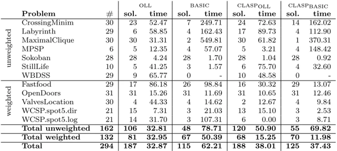
Model Generation. The model generation task is related to SAT solving, and modern ASP solvers are actually based on CDCL-like algorithms [20] properly adapted in order to take into account the properties and the exten-sions of ASP programs. Thus, our system extends the CDCL algorithm by implementing several techniques for handling efficiently specific features of ASP programs, such as minimality of answer sets and inference via aggre-gates. The performances of our implementation have been assessed by an experimental analysis on the instances of the Fourth ASP Competition [23]. The results show that our system is competitive compared with alternative solutions.
Answer Set Checking. The second contribution regards answer set check-ing, which is a co-NP-complete problem for disjunctive logic programs. In fact, a polynomial algorithm for reducing the answer set checking problem into the unsatisfiability problem has been proposed in [27]. However, practi-cal applications have shown the drawbacks of such approach, mostly related to the creation of a new SAT formula for each stability check. We have im-proved the original algorithm by exploiting a strategy based on incremental solving which minimizes the overhead due to multiple calls to an external or-acle. An experimental analysis confirms the viability of our algorithm, which is already comparable with alternative solutions.
Optimum Model Search. Optimum model search is the main task in case of optimization programs in ASP. The task is addressed in this thesis by adapting some of the techniques introduced for MaxSAT solving. In
particular, several algorithms introduced for MaxSAT solving, named mgd [31], optsat [32], pmres [35] and bcd [36] have been properly adapted to the ASP setting. Moreover, the algorithm oll [33] and basic have been also implemented. The former has been introduced for ASP solving and then successfully applied to MaxSAT solving [37], while the latter has been implemented in the ASP solvers smodels [18], dlv [17] and clasp [20].
Cautious Reasoning. Concerning cautious reasoning, we designed and implemented a new framework of anytime algorithms for cautious reasoning in ASP. An algorithm is said to be anytime if it produces valid, intermedi-ate solutions, during its execution, thus it can be safely terminintermedi-ated before the end if the quality of the latest found solution is satisfactory. Our al-gorithms produce certain answers during the computation of the complete solution. The computation can thus be stopped either when a sufficient num-ber of cautious consequences have been produced, or when no new answer is produced after a specified amount of time. Since cautious consequences computation is very hard, anytime property of our algorithms is crucial for real world applications. In fact, we empirically verified that a large number of certain answers can be produced after a few seconds of computation even when the full set of cautious consequences is not computable in reasonable time.
Organization of the Thesis. The remainder of the thesis is organized as follows: In Chapter 2 we describe the techniques originally introduced for SAT solving, which we have been extended to adapt them in a native ASP solver. In Chapter 3 we describe the syntax and semantics of ASP and the use of ASP as a powerful knowledge representation and reasoning tool. In Chapter 4 we describe the solving strategy of new ASP solver and the new algorithm for stable model checking. We also present the results of the exper-iments conducted for assessing the performance of our implementation. In Chapter 5 we compare several strategies for solving ASP optimization prob-lems by introducing several MaxSAT algorithms in the context of ASP. In Chapter 6 we describe algorithms and implementation of cautious reasoning and we show anytime variants of the algorithms reported in literature. In Chapter 7 we describe the work related to this thesis. Finally, Chapter 8 draws the conclusions of the thesis.
Chapter 2
SAT Solving
The Satisfiability (SAT) problem [38] and the Maximum Satisfiability prob-lem are well-known hard probprob-lems. In the recent years effective techniques for solving SAT and MaxSAT have been proposed, and successfully applied to obtain efficient ASP implementations. This chapter provides an overview on the the solving techniques used in modern SAT and MaxSAT solvers. In particular, the classical Davis Putnam Logemann Loveland (DPLL) al-gorithm [39] is presented. After that, its evolution, called Conflict-Driven Clause Learning (CDCL) [40], is described together with some of the tech-niques that are the core of CDCL, such as branching heuristics, learning and restarts. Finally, incremental SAT solving and its usage for solving MaxSAT are recalled.
2.1
The Satisfiability Problem
Let V = {v1, . . . , vn} be a finite set of Boolean variables. A literal ` is a
Boolean variable v or its negation ¬v. Given a literal `, its negation ¬` is ¬v if ` = v and it is v if ` = ¬v. A clause {`1, . . . , `n} is a disjunction of
literals. A SAT instance expressed in Conjunctive Normal Form (CNF) is a conjunction of clauses. A set of literals L is said to be consistent if, for every literal ` ∈ L, ¬` /∈ L holds. An interpretation is a consistent set of literals. Given an interpretation I and a literal `:
• ` is true w.r.t. I if ` ∈ I; • ` is false w.r.t. I if ¬` ∈ I;
A clause {`1, . . . , `n} is said to be satisfied if at least one literal among
`1, . . . , `n is true. A clause is said to be violated if all literals `1, . . . , `n
are false. A clause is undefined if it is neither satisfied nor violated. An interpretation I is a satisfying variable assignment (or model ) for a CNF formula ϕ if all clauses of ϕ are satisfied w.r.t. I. In this case ϕ is said to be satisfiable. Otherwise, if no interpretation is a model of ϕ then ϕ is said to be unsatisfiable. The SAT problem consists of checking whether a given CNF formula ϕ is satisfiable.
Example 1 (Satisfiable CNF formula). Let V = {v1, v2, v3} be a set of
Boolean variables. Consider the following CNF formula ϕ: {v1, v2} {v2, v3}
{v1, v3} {¬v2, v3}
Interpretation I = {v1, ¬v2, v3} is a model for ϕ. C
Example 2 (Unsatisfiable CNF formula). Let V = {v1, v2, v3} be a set of
Boolean variables. Consider the following CNF formula ϕ: {v1, v2} {v2, v3} {v2, ¬v3}
{v1, ¬v2} {¬v2, v3} {¬v2, ¬v3}
The formula ϕ is unsatisfiable because there is no variable assignment that satisfies all the clauses. C
2.2
Davis Putnam Logemann Loveland
Algo-rithm
SAT solving has recently obtained an increasing interest since both indus-trial applications and effective SAT solvers are available. Those results have been obtained as improvements of the Davis Putnam Logemann Lovelang (DPLL) algorithm [39], which is a complete, backtracking-based algorithm for deciding whether a CNF formula is satisfiable or not. DPLL is reported in pseudo-code in Algorithm 1. In a nutshell, the algorithm runs by setting as true an undefined literal `, simplifies the formula accordingly, and then recursively checks whether the simplified formula is satisfiable or not; in the latter case, the same recursive check is done assuming the literal ¬` as true. In more detail, DPLL takes a formula ϕ as input and starts from an assign-ment in which all literals are undefined. Function UnitPropagation (line 2) is invoked in order to satisfy unit clauses. An undefined clause is a unit clause if it contains only one undefined literal. Intuitively, a unit clause can be
Algorithm 1: DPLL
Input : A CNF formula ϕ
Output: True, if ϕ is SAT. False, otherwise.
1 begin
2 ϕ := UnitPropagation(ϕ);
3 ϕ := PureLiteralElimination(ϕ); 4 if all clauses in ϕ are satisfied then 5 return True;
6 if ϕ contains an empty clause then 7 return False;
8 ` = ChooseLiteral();
9 return DPLL(ϕ ∧ `) OR DPLL(ϕ ∧ ¬`);
satisfied only if its unique undefined literal is inferred as true. In practice, unit propagation has a tremendous effect on pruning the search space. Example 3 (Unit clause). Consider the CNF formula ϕ of Example 1 and the interpretation I = {¬v1}. Clause {v1, v2} is unit since there is only one
undefined literal v2. The same consideration holds for clause {v1, v3}. C
After that, function PureLiteralElimination (line 3) is called. This func-tion simplifies clauses containing so-called pure literals. A literal ` is pure if ¬` does not occur in the formula. All clauses in which a pure literal ` appears can be satisfied, and thus deleted, by inferring ` as true. Since ¬` does not appear anyhow in the formula, satisfiability of the remaining clauses is not affected by this operation. However, albeit this optimization is part of the original DPLL algorithm, modern SAT solvers do not implement pure literal checking due to the computational overhead.
Example 4 (Pure literal). Consider the CNF formula ϕ of Example 1. Lit-erals v1 and v3 are pure since ¬v1 and ¬v3 do not occur in ϕ. C
After calling UnitPropagation and PureLiteralElimination, satisfiability of the formula is detected (line 5) if all clauses in ϕ are satisfied; otherwise, if all literals of a clause are false (line 7) then unsatisfiability is detected; finally, if no inferences are possible, an undefined literal `, whose variable is called branching variable, is selected according to a heuristic criterion (line 8), and DPLL is called recursively.
Algorithm 2: Conflict-Driven Clause Learning Input : A CNF formula ϕ
Output: SAT if ϕ is satisfiable, UNSAT otherwise
1 begin
2 while there are undefined clauses in ϕ do 3 ` := ChooseLiteral();
4 ϕ := ϕ ∪ {`};
5 ϕ := UnitPropagation(ϕ);
6 while there are violated clauses in ϕ do 7 ϕ := LearnClause(ϕ);
8 if not RestoreConsistency(ϕ) then 9 return UNSAT;
10 ϕ := UnitPropagation(ϕ); 11 return SAT;
2.3
Conflict-Driven Clause Learning
The original DPLL algorithms described in the previous section has been ex-tended during recent years. In particular, almost all modern SAT solvers are based on a new algorithm, called Conflict-Driven Clause Learning (CDCL) [40]. CDCL is reported in pseudo-code in Algorithm 2. CDCL takes a formula ϕ as input and starts from an assignment in which all literals are undefined. An undefined literal ` is selected according to a branching heuristic criterion. A unit clause {`} is added to the formula ϕ, and UnitPropagation(ϕ) is per-formed as in the standard DPLL. After that, if there are violated clauses in ϕ, function LearnClause(ϕ) is called. This function analyzes violated clauses in order to produce a clause modeling the violation (or conflict) which is added to ϕ (learning). This learned clause is computed in such a way that the variables assignments leading to the violation of the clauses are prohib-ited. Then, the algorithm calls function RestoreConsistency(ϕ) which undoes previous computation until no clauses are violated. If ϕ cannot be consis-tent undoing previous computation, function RestoreConsistency(ϕ) returns false, and the algorithm terminates returning UNSAT. Otherwise, since the learned clause may be unit, function UnitPropagation(ϕ) is invoked, and the learning process is repeated until there are no violated clauses (line 6).
One of the most important features of algorithm CDCL is learning. How-ever, the number of learned clauses can grow exponentially, thus an heuristic for controlling the number of learned clauses is also usually implemented.
Moreover, another important technique usually employed in CDCL is called restarts. Intuitively, some heuristic criteria are used to stop the computation in order to restart the search by taking into account the learned clauses since the first nondeterministic choices.
In the following, we first detail the learning procedure by describing the most used learning scheme. Then, two effective branching heuristics are described in Section 2.3.2. Finally, in Sections 2.3.3 and 2.3.4, some heuristics for deletion of learned clauses and restarts are described, and details are given for those employed by two modern SAT solvers, i.e. minisat [41] and glucose [42].
2.3.1
Learning
Learned clauses forbid literal assignments that are not valid because they lead to a conflict. To perform learning the implication graph is built during unit propagation and a learning scheme is applied [24].
Implication Graph. The implication graph is a directed graph where each node represents a literal that is true with respect to the current assignment. An arc from a node N1 to a node N2 represents that the assignment of N1
participated to the inference of N2, i.e. if N2 is inferred by applying unit
propagation on a clause containing ¬N1. Hence, branching literals have no
incoming edges. When a literal ` is selected by the branching heuristic, a node is added to the implication graph. Each literal ` appearing in the implication graph is associated with a nonnegative integer called decision level, defined as the number of branching literals in the implication graph after literal ` is added. A conflict occurs when the implication graph contains a node for a literal ` and a node for the complementary literal ¬` is added. In this case, literals ` and ¬` are called conflicting literals.
First UIP Learning Scheme. A node N1 with decision level d is said
to dominate a node N2 with the same decision level d if and only if N1 is
contained in all paths connecting the branching literal with decision level d to N2. A Unique Implication Point (UIP) in conflictual implication graph is a
node at the current decision level that dominates both vertices corresponding to the conflicting literals. It is important to note that a UIP represents a unique reason of the current decision level that implies the conflict, and thus, there may be more than one UIP for a certain conflict (e.g. the decision literal is always a UIP). The UIPs are usually ordered starting from the conflict. In the first UIP [26] learning scheme, the learned clause is composed by the
first UIP in the above-mentioned order and by the literals from a smaller decision level that imply the conflict. The first UIP learning scheme usually allows to learn the smallest clauses implying the conflict [26]. The learning algorithm is the following:
1. Let u be the first UIP, and d be its decision level.
2. Let L be the set of literals with decision level d occurring in a path from u to the conflicting literals.
3. Add a literal ` to the learned clause if there is an arc (¬`, `0) in the
implication graph, `0 ∈ L and the decision level of ` is lower than d. 4. Add ¬u to the learned clause.
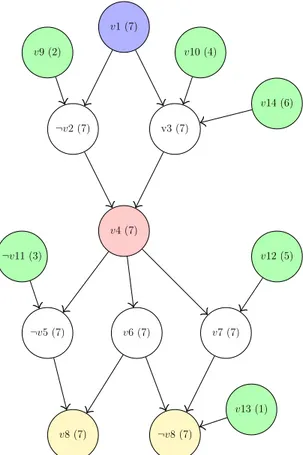
Example 5 (Learning). Consider the following CNF formula ϕ: {¬v1, ¬v9, ¬v2} {¬v1, ¬v10, ¬v14, v3}
{v2, ¬v3, v4} {¬v4, v11, ¬v5} {v6, ¬v4} {¬v4, ¬v12, v7} {v5, ¬v6, v8} {¬v6, ¬v7, ¬v13, ¬v8}
A possible Implication Graph associated to ϕ is shown in Figure 2.1. Decision levels are reported in parentheses. Literal v1 is the branching literal with decision level 7 and leads to the derivation of the literals with decision level 7. The remaining literals v9 to v14 have been assigned as true in a previous decision level. UIPs are v1 and v4, because they are part of all paths from v1 to either v8 or ¬v8. The first UIP is v4, since it is the UIP closest to the conflict. The learned clause is {¬v4, v11, ¬v12, ¬v13}. C
2.3.2
Branching Heuristics
An important role in CDCL, as well as in DPLL, is played by the branching heuristics. In the following we focus on two heuristics that are employed with success in CDCL solvers, namely the Variable State Independent Decaying Sum heuristic and the minisat heuristic.
Variable State Independent Decaying Sum. The Variable State Inde-pendent Decaying Sum (VSIDS) [26] heuristic maintains a counter cl(`) for each literal `. Counters are initialized to 0 and a counter cl(`) is increased when a literal ` appears in a learned clause. Periodically, all counters are divided by a constant. At each decision, the next branching literal is the
v1 (7) ¬v2 (7) v3 (7) v4 (7) ¬v5 (7) v6 (7) v7 (7) v8 (7) ¬v8 (7) v9 (2) v10 (4) ¬v11 (3) v12 (5) v13 (1) v14 (6)
Figure 2.1: Implication Graph (First UIP: v4; Level in parentheses)
undefined literal ` with the highest value of cl(`). If two or more literals have the same highest value of the heuristic counter, the next branching literal is chosen randomly among them.
minisat. The branching heuristic of the SAT solver minisat [41] is an enhancement of the original VSIDS. minisat maintains an activity counter for each variable. The activity counter is initialized to 0. When a variable v is involved in the learning process, i.e. it is responsible of some conflictual assignments, its activity counter of v is increased by an increment value. The increment is initialized to the value 1.0 and it is multiplied by 1.0/0.95 after each conflict. Thus, counters of the variables involved in future conflict will be increased by a higher value. This has the effect to give more importance to variables involved in recent conflicts. At each decision, the variable with the highest activity is chosen as false. Ties are broken randomly.
2.3.3
Learned Clauses Deletion
The number of learned clauses can grow exponentially, and this may cause a performance degradation of propagation. A heuristic is usually employed for deleting some of them. We present the heuristic employed by minisat and glucose, since their effectiveness has been proved in practical applications.
minisat. The SAT solver minisat [41] implements a heuristic that re-moves learned clauses not involved often in recent conflicts. Each learned clause is associated with activity counters measuring the number of times a clause was involved in the derivation of a conflict and are considered locked if binary or when participated to the inference of some literal. Clauses are then deleted performing the following algorithm:
1. Sort all clauses by increasing activity;
2. Remove the first half of the learned clauses that are not locked; 3. Remove all learned clauses that are not locked and have an activity
counter smaller than a threshold.
Glucose. The deletion heuristic of glucose [42] is based on the concept of Literals Blocks Distance (lbd). Given a learned clause c, the lbd of c is the number of different decision levels associated with the literals in c. The lbd is computed when c is learned and it is updated in specific instants of the search. In more detail, the lbd of a clause c is updated when c is involved in the derivation of a new conflict, i.e. when a literal ` ∈ c, inferred by unit propagation through c, is navigated in the implication graph during the computation of a new learned clause.
Clauses are deleted performing the following algorithm: 1. Sort all clauses by increasing lbd.
2. Remove the first half of the learned clauses that are not locked. Thus, clauses with an higher value of lbd are more likely to be deleted in the glucose heuristic.
2.3.4
Restarts
In addition to basic learning, many SAT solvers exploit another technique called restarts, that consists of a halt in the solution process, and a restart of the search. Essentially, the solution process is interrupted, and the search of
Function ChooseLiteral(Set assum∧, Set assum∨) 1 if ∃ an undef ined literal ` ∈ assum∧ then 2 return `;
3 if ∃ a true literal ` ∈ assum∨ then 4 return ChooseLiteral();
5 if ∃ an undef ined literal ` ∈ assum∨ then 6 return `;
7 return ChooseLiteral();
a model is restarted from scratch. We present the restart strategies employed by minisat and glucose.
minisat. The SAT solver minisat performs restarts depending on the number of encountered conflicts and according to a heuristic sequence. In particular, minisat uses the following sequence of conflicts (32, 32, 64, 32, 32, 64, 128, 32, 32, 64, 128, 256, . . . ) which is based on the Luby series introduced in [43].
Glucose. The SAT solver glucose implements a new strategy for restarts considering the lbd scores of learned clauses [44]. In particular, the idea is to restart when learned clauses of recent conflicts are increasing the lbd scores. In more detail, this heuristic has two parameters k and x, which in glucose are set to 0.7 and 100, respectively. The latest x conflicts are considered, and the average of their lbd scores is multiplied by k. A restart occurs when this value is greater than the average lbd of all clauses.
2.4
Incremental SAT
SAT solvers take a CNF formula ϕ as input, then look for a variable assign-ment that satisfies ϕ, and then return SAT if such variable assignassign-ment exists, and UNSAT otherwise. Albeit a single call to a SAT solver is sufficient for many applications, many problems are not efficiently solvable in a unique call. When multiple calls are needed the following naive algorithm can be applied:
1. Create a CNF formula ϕ modeling the problem. 2. Invoke a SAT solver on the CNF formula ϕ.
3. Analyze the results.
4. If a solution to the problem is found then stop.
5. Otherwise create a new CNF formula and go to step 2.
However, this algorithm has shown to be inadequate in many practical cases. The first drawback is that at each iteration the formula is rebuilt. Moreover, the learned clauses cannot be exploited in different iterations. For this reason, modern SAT solvers add an incremental interface for allowing multiple calls. The key idea is to modify the formula ϕ in order to be shared by all calls, and then solve the problem by using a set of literal assumptions [45], which model a particular instance of the problem. In more detail, an incremental variant of Algorithm 2 can be implemented by introducing two sets of assumptions, assum∧ and assum∨. The incremental algorithm checks whether a formula
ϕ is satisfiable under the literal assumptions, that is, if there exists a model of ϕ such that assum∧ and assum∨ are satisfied. Given an interpretation I:
• assum∧ is satisfied if assum∧ ⊆ I, i.e. if each literal ` ∈ assum∧ is
true w.r.t. I;
• assum∨ is satisfied if assum∨ ∩ I 6= ∅, i.e. if at least one literal ` ∈
assum∨ is true w.r.t. I.
The satisfiability test under assumptions can be implemented by modifying the function ChooseLiteral of Algorithm 2 in the following way:
1. If assum∧ is satisfied go to step 2. Otherwise, pick the first undefined
literal among the literals in assum∧.
2. If assum∨ is satisfied go to step 3. Otherwise, pick the first undefined
literal among the literals in assum∨.
3. Pick a branching literal as in the non-incremental algorithm.
The search then runs as in the non-incremental version. If during the search the assumptions assum∧ or the assumptions assum∨ are violated then the
algorithm undoes the computation until the assumptions are not violated anymore.
An important advantage of this incremental strategy is its capability of reusing learned clauses from previous invocations. In a CDCL solver this has a great impact on the performance, since all of the previous computation is used for pruning the search space in future calls. The incremental interface provided by many modern SAT solvers has been used to solve several prob-lems, ranging from MaxSAT to QBF. In the following we show an algorithm for solving the MaxSAT problem based on iterative calls to a SAT solver.
Algorithm 3: Fu&Malik algorithm
Input : A WCNF formula Φ = ϕH ∪ ϕS
Output: An optimum model forΦ
1 begin
2 while true do
3 (res, ϕC, M) := SATSolver(Φ); 4 if res= SAT then return M; 5 S:= ∅;
6 foreach clause c ∈ ϕC ∩ ϕS do 7 let v be a fresh variable; 8 c:= c ∪ {v};
9 S := S ∪ {v};
10 ϕH := ϕH ∪ CN F (#AtM ostOne(S));
2.5
Maximum Satisfiability
The Maximum Satisfiability (MaxSAT) problem is the optimization variant of SAT where clauses are replaced by weighted clauses. A weighted clause is a pair (c, w), where c is a clause and w, called weight, is either a positive integer or >. A weighted clause (c, w) is said to be a hard clause if w = >, otherwise the clause is soft and w represents the cost of violating the clause. A formula in weighted conjunctive normal form (WCNF) Φ = ϕH ∪ ϕS is a
set of weighted clauses, where ϕH is the set of hard clauses, and ϕS is the
set of soft clauses. A model for Φ is a variable assignment I that satisfies all hard clauses. The cost of a model I is the sum of weights of the soft clauses that are violated w.r.t. I. Given a WCNF Φ, the MaxSAT problem is to find a model that minimizes the cost of violated soft clauses in Φ. Several variants of the MaxSAT problem can be obtained by applying constraints to the sets of hard and soft clauses. In particular, given a weighted formula Φ = ϕH ∪ ϕS:
• If ϕH = ∅ and ∀ (c, w) ∈ ϕS, w = 1, the problem is referred to as
(unweighted) MaxSAT.
• If ϕH = ∅ and ∃ (c, w) ∈ ϕS : w > 1, the problem is referred to as
weighted MaxSAT.
• If ϕH 6= ∅ and ∀ (c, w) ∈ ϕS, w = 1, the problem is referred to as
• If ϕH 6= ∅ and ∃ (c, w) ∈ ϕS : w > 1, the problem is referred to as
weighted partial MaxSAT.
During recent years, several algorithms have been proposed for solving the above variants of the MaxSAT problem. Modern and effective MaxSAT solvers implement algorithms that call iteratively a SAT solver and use the incremental interface described in Section 2.4. Many of those algorithms are based on the concept of unsatisfiable core (or simply core) of an un-satisfiable CNF formula ϕ, that is, a subset of ϕ which is still unsatisfi-able. Core-based algorithms have been successfully applied for solving in-dustrial instances as witnessed by the results of the MaxSAT evaluations (see http://maxsat.ia.udl.cat/) and they represent the state-of-the-art of MaxSAT solving. In the following we present the first core-based algo-rithm for partial MaxSAT problems, which has been proposed in [46] and it is called Fu&Malik algorithm. The Fu&Malik algorithm is important for historical reasons since it introduced the concept of unsatisfiable cores for solving the MaxSAT problem. The pseudo code of Fu&Malik algorithm is sketched in Algorithm 3. The algorithm takes as input a WCNF formula Φ = ϕH∪ ϕS and returns as output an optimum model forΦ. The algorithm
uses a modified SAT solver that takes as input a formula Φ and returns as output a triple (res, ϕC, M), where res is a string, ϕC a set of clauses and M
an interpretation. The SAT solver searches for a model ofΦ. If one is found, say M , the function returns (SAT, ∅, M ). Otherwise, the function returns (U N SAT, ϕC, ∅), where ϕC is an unsatisfiable core of ϕC. In the following,
without loss of generality, we assume that ϕH is satisfiable. The Fu&Malik
algorithm algorithm invokes the internal SAT solver on the formula Φ. If a model is found, then the algorithm terminates returning it (line 4). Oth-erwise, an unsatisfiable core ϕC is found. For each soft clause c ∈ ϕC, a
fresh variable v is added to the clause c. The variable v is called relaxation variable, and, intuitively, it can be used for satisfying a soft clause without leading to a conflict. Moreover, the algorithm adds to the formula Φ an ad-ditional set of clauses enforcing that at most one of the relaxation variables is assigned to true (line 10). This set of clauses assures to relax selectively at most one soft clause for each core. The algorithm then iterates until an optimum model is found.
Chapter 3
Answer Set Programming
Answer Set Programming (ASP) [1, 2, 3, 4, 5, 6, 7] is a declarative pro-gramming approach that provides a simple formalism for knowledge repre-sentation. ASP is based on the stable model semantics of logic programs [1] and allows for expressing all problems in the second level of the polynomial hierarchy [2]. In this chapter, we first introduce the syntax and the seman-tics of ASP as background for motivating its applications and to show how it can be used as a powerful knowledge representation and reasoning tool. An architecture of a general system for evaluating ASP programs is then presented.
3.1
Syntax
By convention, strings starting with uppercase letters refer to first-order variables, while strings starting with lower case letters refer to constants. A term is either a variable or a constant. Predicates are strings starting with lowercase letters. An arity (non-negative integer) is associated with each predicate. A standard atom is an expression p(t1, . . .,tn), where p is a
predicate of arity n and t1,. . . ,tn are terms. A standard atom p(t1, . . .,tn) is
ground if t1, . . . , tn are constants.
A set term is either a symbolic set or a ground set. A symbolic set is a pair {T erms : Conj}, where Terms is a list of terms (variables or constants) and Conj is a conjunction of standard atoms, that is, Conj is of the form a1, . . . , an and each ai (1 ≤ i ≤ n) is a standard atom. A ground set is a
set of pairs of the form h¯t : conji, where ¯t is a list of constants and conj is a conjunction of ground atoms. An aggregate function is of the form f(S), where S is a ground set and f ∈ {#count, #sum} is an aggregate function symbol. An aggregate atom is of the form f(S) ≺ T , where f (S) is an
aggregate function, ≺∈ {=, <, ≤, >, ≥} is a predefined comparison operator, and T is a constant referred to as guard.
An atom is either a standard atom, or an aggregate atom. A literal is either an atom a, or its default negation not a. Given a literal ` we will use∼`
for denoting its complement, that is not a if ` = a and a if ` = not a, where a is an atom. This notation extends to sets of literals, i.e., ∼L:= {∼` | ` ∈ L}
for a set of literals L.
Definition 1. A (disjunctive) rule is of the following form:
a1∨ · · · ∨ am ← `1, . . . , `n (3.1)
where a1, . . . , am are standard atoms and `1, . . . , `n are literals, m ≥ 0 and
n ≥ 0.
For a rule r of the form (3.1), disjunction a1∨ · · · ∨ am is called the head of r
and conjunction `1, . . . , `n is named the body of r. The set of head atoms is
denoted by H(r). The set of body literals is denoted by B(r), while the set of positive and negated literals in B(r) are denoted by B+(r) and by B−(r),
respectively. Moreover C(r) := H(r) ∪ ∼B(r) is the clause representation
of r. A rule r is positive if B−(r) = ∅. A normal rule is a rule of the form (3.1) such that m ≤ 1. An integrity constraint, or simply constraint, is a rule of the form (3.1) such that m = 0. A weak constraint is a constraint which is associated with a positive integer by the partial function weight. For a compact representation, the weight will be sometimes indicated near the implication arrow, e.g., ←3 a, not b is a constraint of weight 3. A fact is
a rule of the form (3.1) such that m = 1 and n = 0.
A program ΠR is a set of rules. The set of constraints in ΠR is denoted
constraints(ΠR), while the remaining rules are denoted by rules(ΠR). A
program with weak constraints Π is a pair (ΠR,ΠW), where ΠR is a program
and ΠW is a subset of constraints(ΠR). ΠW is the set of weak constraints,
while constraints(ΠR) \ ΠW is the set of hard constraints. The set of atoms
appearing in ΠR is denoted by atoms(ΠR). A program Π is said to be
dis-junctive if Π contains at least one disjunctive rule. Otherwise, Π is said to be normal. A term, an atom, a literal, a rule, or a program is called ground if no variables appear in it. A local variable of a rule r is a variable ap-pearing only in sets terms of r; a variable of r is global if it is not local. In ASP, rules in programs are required to be safe. A rule r is safe if both the following conditions hold: (i) for each global variable X of r there is a positive standard literal ` ∈ B+(r) such that X appears in `; (ii) each local variable of r appearing in a symbolic set {T erms : Conj} also appears in Conj. A program is safe if each of its rules is safe. In the following, we will only consider safe programs.
Example 6 (Disjunctive logic program). Consider the following disjunctive logic program:
r1 : a(X) ∨ b(X) ← c(X), not d(X)
r2 : ← c(X), f (X)
r3 : c(1) ←
• Rule r1 is a disjunctive rule with H(r1) = {a(X), b(X)}, B+(r1) =
{c(X)}, and B−(r
1) = {d(Y )}.
• Rule r2 is a constraint with B+(r2) = {c(X), f (X)} and B−(r2) = ∅.
• Rule r3 is a fact. Note that every fact must be ground in order to be
safe. C
3.2
Semantics
The answer set semantics is defined on ground programs and it is given by its stable models. Given a programΠ, the Herbrand universe UΠis the set of all
constants appearing in Π. If there are no constants in Π, then UΠ contains
an arbitrary constant c. Given a program Π, the Herbrand base BΠ is the
set of all possible ground atoms which can be constructed from the predicate symbols appearing in Π with the constants of UΠ.
Example 7 (Herbrand universe and Herbrand base). Consider the following program Π0:
r1 : a(X) ∨ b(X) ← c(X)
r2 : d(X) ← b(X), c(X)
r3 : c(1) ←
r4 : c(2) ←
Then, UΠ0 = {1, 2} and BΠ0 = {a(1), a(2), b(1), b(2), c(1), c(2), d(1),
d(2)}.C
For any rule r, Ground(r) denotes the set of rules obtained by replacing each variable in r by constants in UΠ in all possible ways. For any programΠ, its
ground instantiation is the set Ground(Π) = S
r∈ΠGround(r) 1.
Example 8 (Ground instantiation). Consider the programΠ0 in Example 7.
Its ground instantion is the following:
g1 : a(1) ∨ b(1) ← c(1) g2 : a(2) ∨ b(2) ← c(2) g3 : d(1) ← b(1), c(1) g4 : d(2) ← b(2), c(2) g5 : c(1) ← g6 : c(2) ←
Note that the atoms c(1) and c(2) are already ground in Π0, while the rules
g1 and g2 are obtained from r1 and the rules g3 and g4 are obtained from
r2.C
A set L of ground literals is said to be consistent if, for every literal ` ∈ L, its complementary literal ∼` does not belong to L. An interpretation I for
Π is a consistent set of ground literals over atoms in BΠ. A ground literal `
is interpreted as follows: • ` is true w.r.t. I if ` ∈ I. • ` is false w.r.t. I if ∼` ∈ I.
• ` is undefined w.r.t. I if it is neither true nor false w.r.t. I.
A ground conjunction of atoms conj is true w.r.t. I if all atoms appearing in conj are true w.r.t. I. Conversely, conj is false w.r.t. I if there is an atom in conj that is false w.r.t. I. Let I(S) denote the multiset [ t1 | ht1, . . . , tni :
conj ∈ S ∧ conj is true w.r.t. I ]. The valutation I(f (S)) of an aggregate function f(S) w.r.t. I is the result of the application of f on I(S) [8]. Let r be a rule in Ground(Π).
• The head of r is true w.r.t. I if and only if there is an atom a ∈ H(r) such that a is true w.r.t. I.
• The body of r is true w.r.t. I if and only if each literal ` ∈ B(r) is true w.r.t. I.
• The head of r is false w.r.t. I if and only if each atom a ∈ H(r) is false w.r.t. I.
• The body of r is false w.r.t. I if and only if there is a literal ` ∈ B(r) such that ` is false w.r.t. I.
A rule r is satisfied w.r.t. I if and only if H(r) is true w.r.t. I or B(r) is false w.r.t. I. For a rule r, I |= r if r is satisfied w.r.t. I.
An interpretation I is total if and only if for each literal ` ∈ BΠ, ` ∈ I
or ∼` ∈ I, otherwise I is partial. A total interpretation M is a model for
Π if and only if for each rule r ∈ Π, M |= r. Stated differently, a total interpretation M is a model for Π if, for each r ∈ Π, r is satisfied w.r.t. M . A model M is a stable model (or answer set ) for a positive programΠ if it is a minimal set (w.r.t. set inclusion) among the models for Π. The definition of stable models for general programs is based on the FLP-reduct [8]. Definition 2. The FLP-reduct [8] of a ground program Π w.r.t. an inter-pretation I is the ground program ΠI obtained from Π by deleting each rule
r ∈ Π whose body is not satisfied w.r.t. I.
Definition 3. A stable model (or answer set ) [1] of a program Π is a model I of Π such that I is a stable model of ΠI.
Let SM(Π) denote the set of stable models of Π. If SM (Π) 6= ∅ then Π is coherent, otherwise it is incoherent.
Definition 4 (Optimum Stable Model). For a program with weak constraints Π = (ΠR,ΠW), each interpretation I is associated with a cost:
cost(ΠW, I) :=
X
r∈ΠW : I6|= r
weight(r).
A stable model I ofΠR\ΠWis optimum forΠ if there is no J ∈ SM (ΠR\ΠW)
such that cost(ΠW, J) < cost(ΠW, I).
An atom a ∈ atoms(Π) is a cautious consequence of a program Π if a belongs to all stable models ofΠ. More formally, a ∈ atoms(Π) is a cautious consequence of a program Π there is no M ∈ SM (Π) such that a /∈ M . The set of cautious consequences of Π is denoted CC(Π).
3.3
Properties of ASP programs
In this section we recall some properties of answer sets.
Definition 5 (Supportedness Property). Given an interpretation I, a positive literal ` is supported w.r.t. I if and only if there exists a rule r such that for each literal `b is true with respect to I and for each atom `h ∈ H(r) \ {`},
A model M is said to be supported if for each positive literal a ∈ M , a is supported. Answer sets are supported models, while the reverse is not necessarily true.
Definition 6 (Possibly Supporting Rule). Given an interpretation I, a rule r is a possibly supporting rule for an atom a if the following conditions hold:
• a ∈ H(r); and
• no literal in B(r) is false with respect to I; and • (H(r) \ {a}) ∩ I = ∅.
Let supp(a, I) denotes the set of possibly supporting rules for an atom a and an interpretation I.
Definition 7 (Dependency Graph). Let Π be a program. The dependency graph of Π, denoted DGΠ = (N, A), is a directed graph in which (i) each
atom in atoms(Π) is a node in N and (ii) there is an arc in A directed from a node a to a node b if there exists a rule r in Π such that a ∈ H(r) and either b ∈ B+(r) or b occurs in an aggregate atom. It is important to note that negative literals cause no arc in DGΠ. We also safely assume that any
rule r such that H(r) ∩ B+(r) 6= ∅ is removed from Π.
Definition 8 (Component). A strongly connected component (or simply component ) C of DGΠ is a maximal subset of N such that each node in
C is connected by a path to all other nodes in C.
In the following, we assume that for each rule r, and for each pair of atoms (a,b) such that a ∈ H(r) and b appears in aggregate atom of r, a and b are in two different components.
A component C is recursive, or cyclic, if C contains two or more atoms. A component C is head-cycle free (HCF for short) if each rule r ∈ Π is such that |H(r) ∩ C| ≤ 1. Otherwise C is said to be non head-cycle free (non-HCF). Given a program Π, the subprogram sub(Π, C) corresponding to a component C of the dependency graph is defined as the set of rules r ∈ Π such that H(r) ∩ C 6= ∅. The rules of Π can be assigned to one or more components. More specifically, a rule r is assigned to a component C if r ∈ sub(Π, C). Moreover, a rule r ∈ sub(Π, C) is said to be an external rule of C if B+(r) ∩ C = ∅; otherwise, r is an internal rule of C. An atom a
is said to be an external atom of C if a /∈ C; otherwise, the atom is internal. A literal ` = a or ` = ∼a is said to be an external literal if a is an external
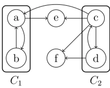
a b e f c d C1 C2
Figure 3.1: Dependency graph of the program Π
Example 9. Consider the following program Π:
r1 : a ← e r5 : c ← a, e
r2 : a ← b r6 : c ← d
r3 : b ← a r7 : d ← c
r4 : e ∨ f ← r8 : c ∨ d ← f
The dependency graph DGΠ of Π is reported in Fig. 3.1, where we also
represented the two recursive components C1 = {a, b} and C2 = {c, d}. The
component C1is HCF; r1is an external rule, while rules r2and r3are internal.
The component C2 is non-HCF; r5 and r8 are external rules, while rules r6
and r7 are internal. C
Definition 9 (Unfounded Set). A set X of atoms is unfounded w.r.t an interpretation I if for each rule r such that H(r) ∩ X 6= ∅, at least one of the following conditions is satisfied:
i) The body of r is false w.r.t I.
ii) The body of r is false w.r.t. (I \ X) ∪∼X.
iii) ((H(r) \ X) ∩ I) 6= ∅, that is, there exists a true atom w.r.t. I in the head of r that does not belong to X.
Theorem 1 (Theorem 4.6 in [48]). Let Π be a program and I a supported model for Π, I is an answer set iff I is unfounded-free, i.e. if there exists no non-empty X ⊆ I such that X is an unfounded set for Π w.r.t. I [48].
The unfounded-free property can be verified independently for each com-ponent C of the program, i.e. an interpretation I is unfounded-free w.r.t. a program Π iff I is unfounded-free w.r.t. each subprogram sub(Π, C). Check-ing whether a set of atoms is unfounded is known to be polynomial for HCF components, while it is a co-NP complete problem for non-HCF compo-nents [2].
Definition 10 (Rule shifting). Let r be a disjunctive rule of the form a1∨
· · · ∨ am ← `1, . . . , `n. The shifting of r consists of replacing r by m normal
rules, one for each atom in the head. The rule for the i-th head atom is as follows:
ai ← `1, . . . , `n, not a1, . . . , not ai−1, not ai+1, . . . , not am. (3.2)
Definition 11 (Clark’s Completion). Given a ground program Π, let auxr
denotes a fresh atom, i.e., an atom not appearing elsewhere, added for a rule r ∈ Π. The Clark’s completion (or completion) of Π, denoted Comp(Π), consists of the following set of rules:
← not a, auxr1
. . .
← not a, auxrn
← a, not auxr1, . . . , not auxrn
for each atom a ∈ atoms(Π), where r1, . . . , rnare the rules in Π whose heads
contain a.
← not auxr, B(r)
for each rule r ∈Π;
← auxr,∼bi
for each rule r ∈Π and for each bi ∈ B(r);
Example 10. Consider the following program Π: r1 : a ∨ b ←
r2 : c ∨ d ← a
The program Π after shifting disjunctive rules is the following: r1 : a ← not b r2 : b ← not a
r3 : c ← a, not d r4 : d ← a, not c
Finally, Comp(Π) consists of the following set of rules: ← not a, auxr1 ← not b, auxr2
← not c, auxr3 ← not d, auxr4
← a, not auxr1 ← b, not auxr2
← c, not auxr3 ← d, not auxr4
← not auxr1, not b ← not auxr2, not a
← not auxr3, a, not d ← not auxr4, a, not c
← auxr1, b ← auxr2, a
← auxr3, not a ← auxr4, not a
Proposition 1. If M is a model of Comp(Π) then M |Π is a supported
model of Π, where M |Π is the restriction of M to the symbols of Π, that is,
M |Π:= M ∩ atoms(Π).
3.4
Knowledge Representation And Reasoning
ASP can be used to encode problems in a simple and declarative way. More-over, ASP is very expressive by allowing to represent problems that belong to the complexity class ΣP
2 (i.e. N PN P). The simplicity of encodings and
the high expressivity of the language are the keys of the success of ASP. In fact, ASP has been used in several domains, such as artificial intelligence, deductive databases, bioinformatics, and also on industrial problems.
In this section, we show the usage of ASP as a tool for knowledge repre-sentation and reasoning by examples. In particular, we present three well-known problems: 3-Colorability, Consistent Query Answering and Maximum Clique. The problem 3-Colorability shows how hard problems can be easily encoded in ASP; Consistent Query Answering shows an application of cau-tious reasoning in ASP; and the problem Maximum Clique shows how ASP can deal with optimization problems by means of weak constraints.
NP-problems are usually encoded in ASP by using the “Guess & Check” methodology originally introduced in [49] and refined in [17]. The idea behind this method can be summarized as follows: a set of facts (input database) is used to specify an instance of the problem, while a set of rules (guessing part), is used to define the search space; solutions are then identified in the search space by another set of rules (checking part), which impose some admissibility constraints. In other words, the guessing part with the input database defines the set of all possible solutions, which are then filtered by the checking part to guarantee that the answer sets of the resulting program represent precisely the admissible solutions for the input instance.
3-Colorability. Given a finite undirected graph G = (V, E) and a set of three colors C, does there exist a color assignment for each vertex such that there are no adjacent vertices sharing the color assignment?
This is a typical NP-complete problem in graph theory. Suppose that the graph G is specified by using facts over predicates vertex and edge. Then, the following program solves the Graph Coloring problem:
r1 : col(X, ”blue”) ∨ col(X, ”red”) ∨ col(X, ”green”) ← vertex(X)
r2 : ← edge(X, Y ), col(X, C), col(Y, C)
This NP-complete problem is encoded in a simple way by using the “Guess & Check” methodology. In the example, the guessing part is composed by
the rule r1 while the rule r2 composes the checking part. In fact, r1 guesses
a color assignment for a vertex v and r2 checks whether the color assignment
is valid assuring that two adjacent vertices have different color assignments.
Consistent Query Answering. Consistent Query Answering (CQA) is a well-known application of ASP [28, 50]. Consider an inconsistent database D where in relation R = {h1, 1, 1i, h1, 2, 1i, h2, 2, 2i, h2, 2, 3i, h3, 2, 2i, h3, 3, 3i} the second argument is required to functionally depend on the first. Given a query q over D, CQA amounts to computing answers of q that are true in all repairs of the original database. Roughly, a repair is a revision of the original database that is maximal and satisfies its integrity constraints. In the example, repairs can be modeled by the following ASP rules:
r1: Rout(X, Y1, Z1) ← R(X, Y1, Z1), R(X, Y2, Z2), Y16= Y2, not Rout(X, Y2, Z2)
r2: Rin(X, Y, Z) ← R(X, Y, Z), not Rout(X, Y, Z)
Rule r1 detects inconsistent pairs of tuples and guesses tuples to remove in
order to restore consistency, while r2 defines the repaired relation as the set
of tuples that have not been removed. The first and third arguments of R can thus be retrieved by means of the following query rule:
q1: Q(X, Z) ← Rin(X, Y, Z)
The consistent answers of q1 are tuples of the form hx, zi such that Q(x, z)
belongs to all stable models. In this case the answer is {h1, 1i, h2, 2i, h2, 3i}.
Maximum Clique. Given a finite undirected graph G = (V, E), a clique C is a subset of its vertices such that for each pair of vertices in C an edge connects the two vertices. The Maximum Clique problem is to find a clique with the greatest cardinality. That is, for each other clique C’ in G, the number of nodes in C should be larger than or equal to the number of nodes in C’.
Suppose that the graph G is specified by using facts over predicates vertex and edge. Then, the following program solves the Maximum Clique problem:
r1: in(X) ∨ out(X) ← vertex(X)
r2: ← in(X), in(Y ), not edge(X, Y ), not edge(Y, X), X < Y
r3: ←1out(X)
This program shows the encoding of optimization problems by means of weak constraints. In the example, rule r1 represents the guessing part while the
rule r2 composes the checking part. In fact, r1 guesses a subset of nodes
candidates to be in a clique and rule r2 checks whether the subset of nodes is
a clique assuring that every vertices in the clique are connected by an edge. Finally, rule r3 minimizes the number of nodes which are not in the clique.
3.5
Architecture of an ASP System
The architecture of an answer set system is usually composed by three mod-ules. The first module is the Grounder, which is responsible of the creation of a ground program equivalent to the input one. After the grounding process, the next module, usually called Model Generator, computes stable model candidates of the program. Stable model candidates are, in turn, checked by the third module, called Answer Set Checker, which verifies that candidates are actually stable models. These three modules are briefly described in this section.
Grounder. Given an input programΠ, the Grounder efficiently generates an intelligent ground instantiation of Π that has the same answer sets of the theoretical instantiation, but is usually much smaller [17]. Note that the size of the instantiation is a crucial aspect for efficiency, since the answer set computation takes exponential time (in the worst case) in the size of the ground program received as input (i.e., produced by the Grounder). In order to generate a small ground program equivalent to Π, the Grounder gener-ates ground instances of rules containing only atoms which can possibly be derived from Π, and thus (if possible) avoiding the combinatorial explosion which can be achieved by naively considering all the atoms in the Herbrand base [51]. This is obtained by taking into account some structural informa-tion of the input program concerning the dependencies among predicates, and applying sophisticated deductive database evaluation techniques. An in-depth description of a Grounder module is out of the scope of this thesis. Therefore, we refer the reader to [17, 47] for an accurate description.
Model Generator. The Model Generator takes as input a propositional ASP program and returns as output answer set candidates. The Model Generator usually implements techniques introduced for SAT solving, such as learning, restarts and conflict-driven heuristics. Those techniques match the working principle of a Model Generator but require quite a lot of adaptation to deal with disjunctive logic programs under the stable model semantics.
Answer Set Checker. The goal of the Answer Set Checker is to verify whether a model is an answer set for an input program Π. This task is very hard in general, because checking the stability of a model is well-known to be co-NP-complete [2] in the worst case. In case of hard problems, this check can be carried out by translating the program into a SAT formula and checking whether it is unsatisfiable.
Chapter 4
The ASP Solver wasp 2
This chapter describes the ASP solver for propositional programs wasp 2 [52]. wasp 2 is inspired by several techniques that were originally introduced for SAT solving, like the CDCL algorithm [40], learning [24], restarts [25] and conflict-driven heuristics [26]. The mentioned SAT solving methods have been adapted and combined with state-of-the-art pruning techniques adopted by modern native ASP solvers [53, 54]. In particular, the role of Boolean Constraint Propagation in SAT solvers is taken by a procedure combining the unit propagation inference rule with inference techniques based on ASP program properties. In fact, support inferences are implemented via Clark’s completion, and the implementation of the polynomial unfounded-free checks is based on source pointers [18]. In wasp 2 stability of answer sets is checked by means of a reduction to the unsatisfiability problem as described in [27]. In this chapter, after introducing the architecture of the new solver, we detail the techniques for addressing the tasks of Model Generation and Answer Set Checking as implemented in wasp 2. Finally, we report on an experimental analysis in which we assess the performance of our solutions compared to the state-of-the-art alternatives.
4.1
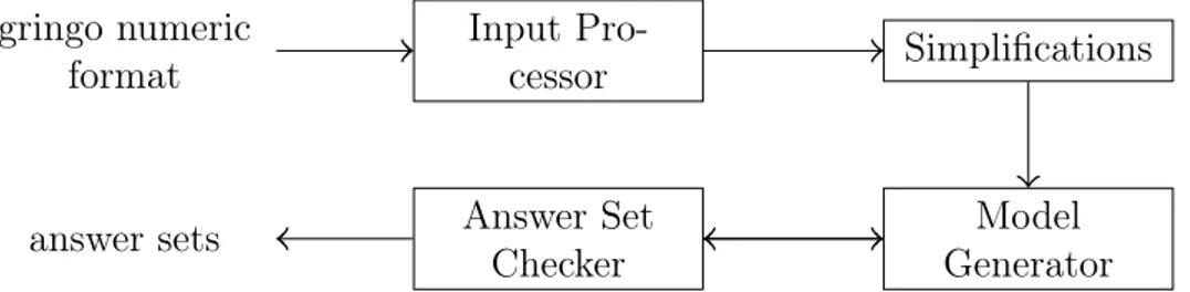
The Architecture of wasp 2
The architecture of wasp 2 is composed by four modules, and it is shown in Figure 4.1. The first module is the Input Processor, which takes as input a ground program encoded in the numeric format of gringo [47]. The Input Processor applies some preliminary program transformations, and creates the data structures that are used by the subsequent modules. The Simplifications step further modifies the input program by removing redundant clauses and variables. The simplified program is fed as input to the Model Generator
Input Pro-cessor Simplifications Model Generator Answer Set Checker gringo numeric format answer sets
Figure 4.1: Architecture of wasp 2
module, which computes answer set candidates. The subsequent Answer Set Checker module implements a stability check to verify that the produced candidates are in fact answer sets.
4.2
Input Processor
The Input Processor takes as input a ground program encoded in the nu-meric format of gringo and creates the data structures that are employed by the subsequent simplification step. In particular, the Input Processor simplifies its input by removing duplicated and trivial rules, determines a splitting of the program in components (or program modules) and, then, ap-plies two transformations, namely program shifting and Clark’s completion as described in Chapter 3.
Program shifting allows to handle disjunctive programs, and Clark’s com-pletion is applied to take into account the supportedness property of answer sets. Indeed, it follows from Proposition 1 that given an input programΠ the models of Comp(Π) are supported models of Π. This is done for simplifying the architecture of wasp 2 as it is explained in the following.
4.3
Simplifications of the Input Program
Program shifting and Clark’s completion may cause a quadratic blow-up in the size of the input program. Thus, reducing the size of the resulting pro-gram can be crucial for the performance of ASP solvers. The simplifications employed by wasp 2 consist of polynomial algorithms for strengthening and for removing redundant rules, and also include atoms elimination by means of rewriting in the style of satelite [55]. Albeit the size of a program is not always related to the easiness of producing answer sets, program simplifica-tions have a great impact in performance as it happens in SAT solving [55].
In the following we detail the simplifications applied by wasp 2.
Subsumption. Given a program Π and the program Comp(Π) represent-ing the Clark’s completion of Π, wasp 2 implements two types of rule sim-plifications: subsumption and self-subsumption.
Definition 12. A rule r1 ∈ Comp(Π) subsumes a rule r2 ∈ Comp(Π) if
C(r1) ⊆ C(r2), where C(r1) and C(r2) denote the clause representation of r1
and r2, respectively.
A subsumed rule in Comp(Π) is redundant and can be safely removed. Definition 13. A rule r1 ∈ Comp(Π) self-subsumes a rule r2 ∈ Comp(Π)
if there is a literal ` such that ` ∈ C(r1), ∼` ∈ C(r2) and C(r1) \ {`} ⊆
C(r2) \ {¬`}.
Stated differently a rule r1 ∈ Comp(Π) self-subsumes a rule r2 ∈ Comp(Π),
if r1 almost subsumes r2 except for one literal ∼` ∈ C(r2) and ` appears in
C(r1). In this case, the rule r2 can be strengthened by removing ∼`.
Thus, wasp 2 removes subsumed rules of Comp(Π) and then applies self-subsumption to the remaining rules. Subsumption and sulf-self-subsumption are then alternated until no other simplifications can be applied.
Literals Elimination. wasp 2 also implements a procedure for eliminat-ing literals through rule distribution. The procedure detects a definition of a literal `, that is ` ⇐⇒ `1∧ . . . ∧ `n. In particular, a literal ` is eliminated
by rule distribution if the following set of rules exists: ←∼`, `1, . . . , `n
← `,∼`1
. . . ← `,∼`n
Each occurrence of ` is substituted by `1∧ . . . ∧ `n, and each occurrence of∼`
is substituted by `1∨ . . . ∨ `n. However, wasp 2 actually eliminates literals
only if the number of rules after the simplification is less than the original number of rules. Moreover, a literal `= a or ` = not a is not eliminated if a is in a cyclic component or a is an aggregate atom.
4.4
Model Generator
The Model Generator implements a CDCL-like algorithm (see Section 2.3). A pseudo-code description of the Model Generator of wasp 2 is shown in