Aggregate structures analysis of bitumen for the production of modified benders in asphalt industry

Contents.

Abstract……….. I

Introduction……… II

1. Bitumen Production, Structure and Composition……….. 1

1.1 Production ……… 1

1.2 Physical and chemical properties of Bitumen……….. 2

1.3 SARA fractions ……….. 4

1.3.1 Saturates ……….. 6

1.3.2 Aromatics……….. 6

1.3.3 Resins……… 6

1.3.4 Asphaltenes……….. 7

1.4 Sol and Gel bitumens and bitumen modeling……….. 8

1.4.1 The homogeneous model……….. 10

1.4.2 The colloidal model………. 10

1.5 Bitumen ageing……….. 14

1.5.1 Effects of bitumen ageing on its mechanical properties……….. 16

References Chapter 1……… 17

2. Rheology, Nuclear Magnetic Resonance and Atomic Force Microscopy………. 21

2.1 Fundamentals Rheology of Viscoelastic Matter……… 21

2.1.2 Shear rheometry………. 26

2.1.3 Former evaluation of bitumen rheology and current empirical tests… 32 2.2 Nuclear Magnetic Resonance……… 35

2.2.1 Basic Concepts……….. 35

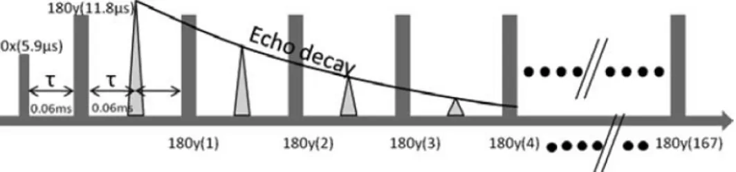
2.2.2 Spin-Spin Relaxation time measurement: Spin Echo Sequences………… 38

2.2.3 Inverse Laplace Transform of the echo decay………. 40

2.3 Atomic Force Microscopy (AFM)………. 42

References Chapter 2……….. 44

3. Additives for Bitumen Recycling and bitumen modifiers……… 47

3.1 Introduction……… 47

3.2 Recycling……….. 48

3.2.1 Recycling methods……… 49

3.2.2 Cold recycling………..50

3.2.3 Hot Recycling………. 51

3.2.4 Warm Mix Asphalt……… 53

3.2.5 Additives……….. 54

3.3 Bitumen Modifiers: Overview……….. 57

3.3.1 Most Used Modifiers……….. 59

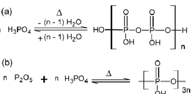
3.3.3 Synthesis, composition and PPA dissociation………. 60 3.3.4 Polyphosphoric acid modified bitumen: proposed mechanisms……….. 62 3.3.5 Crumb rubber modified bitumen……….. 64 References chapter 3……… 65 4. Results part I - Analysis of the effects of bitumen modifiers and additives for

bitumen recycling: Published Data………. 68 5. Results part II - Analysis of the effects of bitumen modifiers and additives for

bitumen recycling: Data to be published……… 70 6. Results part III – Published Papers not related to the doctoral project……… 92

I Abstract

Since antiquity bitumen had been used as a construction material. Nowadays, most of the huge global production of bitumen each year, are functional to the roads paving industry where they are employed as binders for mineral aggregates to produce asphalt mixes. In the paving industry, a suitable bitumen should be fluid enough at to be pumpable and workable for a uniform covering of the mineral aggregates upon amalgamation. Furthermore, once the asphalt has been laid to build the roads, bitumen has to become sufficiently rigid at the highest pavement temperature to oppose rutting, depending on local climate conditions. Conversely, it must stay flexible enough at the lowest pavement temperature to resist cracking. For these purposes, additives such as polymers, acids, etc., are used to calibrate the operative range of bitumen. In addition asphalt industry is interested to reduce the costs of production, the environmental impact of the production and the safety condition for the paving workers. Bitumen is currently modeled as a dispersion of colloidal particles of asphaltenes, surrounded by a layer of stabilizing polar resins in a continuous oil phase (maltene). Although one can write a very simple definition of bitumen, its chemical composition is very complex and still not completely known. However the characterization of the bituminous materials for its convenient application, is still made by empirical standardized tests. This research project aimed to the deeper understanding of the behavior of bituminous systems, in order to correlate the macroscopic properties to the microstructure of the aggregates that constitute the bitumen colloidal network. We explored the possibility of taking advantage from chemical-physics techniques such as NMR, Rheology and AFM. In particular we have investigated the effect and overall the mechanism through which some chemical additives, already in use by paving companies, explicate their action to modulate the bitumen performances. Several samples different in nature and differently modified were analyzed. The rheological analysis, performed by the measurements under kinematic and dynamic control, helped to determine the material properties related to the structure of the system. The parameters thus obtained, being independent of the measurement conditions may be correlated with the microstructure of the sample investigated by the other techniques we used. As for NMR we exploited the spin-spin relaxation time measurement firstly to find the soften point of bituminous materials whether modified or not. As a novel approach to the understanding of the colloidal nature of the bitumen, the Inverse Laplace Transform (ILT) of the NMR spin-echo decay (T2) was applied. The ILT was used to draw the map of the macro-aggregates inside bitumen at different temperatures providing indication on the nature of the interaction between additives and the colloidal network. The efficiency of the ILT method was proved by atomic force microscopy images. As matter of fact collecting the AFM analysis, the ILT and the rheological results, we were able to describe the correlation between the aggregates at supra-molecular level inside fresh and doped bitumen. This research constituted a new inside bitumen chemistry overcoming the limits of the empirical tests to verify the efficiency of the bitumen modifiers.

INTRODUCTION

In the last years, hundreds of new roads were built over the world in order to satisfy the growing traffic load. However many of the existing roads are in use since more than 20 years and the volume of vehicles has noticeably increased. For these two main reasons an increase in roads maintenance is required. In this particular historical moment with one of the worst financial crisis after the second world war, it is not easy to rise adequate funds for roads maintenance leading to a quick deteriorated asphalt pavement. Hence it is essential to innovate and find alternative processes to build up asphalt roads. Recycling aged road pavements is one of this methods. The main points for recycling asphalts are: Reduction of the raw materials; reduction of wasting areas; reduction of pollution; energy saving; economical convenience. Bitumen is the crucial component used for the road constructions in the world, as it is the typical binder adopted for road asphalt conglomerate and, being the only deformable component, it is the main responsible for pavement performance. It is a dark brown to black, cement-like semisolid or solid or viscous liquid produced by the non-destructive distillation of crude oil during petroleum refining. It can also be found in nature as “natural asphalt”. The chemical composition and mechanical properties of bitumen strongly depend on the origin of the crude oil . Indeed bitumen is a complex chemical mixture of molecules that are predominantly hydrocarbons of different molecular sizes with a small amount of structurally analogous heterocyclic species (heteroatoms) and functional groups containing sulphur, nitrogen and hydrogen atoms . Metals like nickel, iron and vanadium are also present. However the elemental analysis is very similar for all the bitumen with a prevalence of hydrocarbons that have a number of carbon atoms higher than 25. Due to this complex chemical composition, bitumen is currently classified for the convenient use by means of empirical standardized tests that were defined since the early 1970s under the USA project SHRP (strategic highway research project). However a more analytical approach is needed to obtain a real improvement of the recycling process and bitumen performance. Hence a better depiction of the molecular and supra-molecular structure of bitumen is essential to understand the action of some additives already in use and to design new ones. Bitumen is currently modeled as a colloidal

dispersion of asphaltene particles, coated with layers of stabilizing polar resins, in a continuous oil phase. Basically it can be viewed as a two phase material with no distinct boundaries between the two fractions. For this reason the mechanical properties of bitumen are the result of the chemical composition and phases arrangement of the molecular structures. This thesis deals with the chemical-physics modification of bitumen binders that produce changes in the supra-molecular arrangement. These changes in turn are reflected on the mechanical properties. In this view we investigated the action of the polyphosphoric acid (PPA) as modifier, that is employed to obtain stiffer binders. However we focused our efforts on the recycling process of bitumen that loses elasticity with aging. This is mainly due to the oxidation of aromatic compounds and resins. Some of the additives already employed by manufacturers to rejuvenate aged bitumen were investigated and their action revealed. To reach this goal we exploited rheology, atomic force microscopy, nuclear magnetic resonance with inverse Laplace transform.

1

1. Bitumen Production, Structure and Composition.

1.1 Production.

In the early 20th century, bitumen was only taken from natural sources [1]. Nowadays, it is basically obtained by the distillation of crude oil [2,3]. Only one tenth of the available crude oil is suitable to yields adequate amounts of bitumen. More or less, the heavier the petroleum, the higher its bitumen amount [2,3]. Native bitumen is poorly used in the paving industry, normally as an additive for other derivated bitumen [4].The distillation (Figure 1.1) is made by separating the light components from the crude oil by atmospheric distillation at about 350 °C. In a successive step, the residue is further refined at a slightly higher temperature (350–425 °C) under vacuum with [5]. The resulting material properties, depend on the crude origin and real operating conditions. Usually, refiners manufacture only a soft and a hard bitumen, and the intermediate are obtained by blending them [2]. When new vacuum distillation columns came with structured packing internals, harder grades can now be obtained by distillation [4].

2 Furthermore another multigrade bitumen, can have a wider operating temperature range than normal bitumen and can be also obtained through acid modification. Other techniques still exist to obtain bitumen from petroleum. Air-blowing was the first process that allowed the manufacture of bitumen from a very fluid crude oil [5,6]. the oil (or soft bitumen) is air-oxidized at 200–275 °C, sometimes in the presence of a catalyst [2]. The properties of the oxidized material, depend on the crude oil origin (or the soft bitumen) and the operating conditions, temperature and time. It still is the best process to make very hard bitumens, especially for waterproofing. However they are not in use for paving applications, because they were too vulnerable to cracking [4]. When a soft bitumen is gently blown to pass paving specifications, the corresponding bitumen is sometimes called semi-blown bitumen.

Another process of minor commercial meaning is the so-called solvent deasphalting, [2]. The heavy fraction of a crude oil (or soft bitumen) is added with 3–10 times its volume of liquid propane and then left to settle [10]. Characteristic conditions are a temperature in the 25–70 °C range and a pressure of 12 bars to maintain propane in the liquid state. The precipitate is bitumen. It still is a good way for recovering lubricants, and the bitumen is a by-product [5,6].

1.2 Physical and chemical properties of Bitumen.

A natural source of heavy crude oil is called bitumen when its density go over 1 g/cm3 at 15.6 °C. However density of bitumen at room temperature is between 1.01 and 1.04 g/cm3, depending on the oil source and paving grade [3]. Normally, the harder it is, the denser the bitumen. Bitumen has a glass transition around −20 °C, although it varies in a range from +5 °C down to −40 °C again depending on the crude origin and somewhat on the process [7,8]. Hence from a thermodynamical point of view, bitumen is a very viscous liquid at room temperature. The complexity of bitumen chemistry lies in the fact that many different chemicals are present. In general the chemical nature of the crude oil is described as paraffinic, naphthenic or aromatic if a majority of saturate, cyclic or aromatic structures, respectively, are present [5]. This classification of the petroleum is sometimes applied to the corresponding bitumen. For example, Venezuelan bitumens are generally known as naphthenic bitumens. The elemental composition of a bitumen depends primarily on its crude source and it is difficult to give geographical generalization [3,9]. For instance materials from the USA or Canada can have quite different compositions. Indeed the first systematic classification of bitumen came with the extraordinary work on bitumen chemistry, structure and properties realized in the USA as part of the Strategic Highway Research Program (SHRP) in the late 1980s [10]. From this data bitumen mainly consists in carbon (typically 80–88 wt.%) and hydrogen atoms (8–12 wt.%). This gives a hydrocarbon

3 content generally superior to 90wt.% with an hydrogen-to-carbon molar ratio H/C around 1.5. This H/C ratio is therefore intermediate between that of aromatic structures (benzene has H/C=1) and that of saturate alkanes (H/C =2) [3,11] . In addition, heteroatoms such as sulphur (0–9 wt.%), nitrogen (0– 2 wt.%) and oxygen (0– 2 wt.%) are generally present. Traces of metals are also found, the most numerous being typically vanadium, and nickel (up to 200 ppm) [3,5,8,11]). Sulfur is generally the most present polar atom. It appears in the form of sulfides, thiols and, to a lesser extent, sulfoxides (Figure 1.2). Oxygen is typically present in the form of ketones, phenols and, to a lesser extent, carboxylic acids (Fig. 2). Nitrogen exists typically in pyrrolic and pyridinic structures and also forms amphoteric species such as 2-quinolones [3,5] (Figure 1.2). Most of the metals form complexes such as metalloporphyrins [5].

Figure 1.2. Classes of chemicals species present in bitumen binder.

Given the concentration of polar atoms, functional groups generally do not amount for more than a few 0.1 mol/l for straight run bitumens [11]. The number-average molecular weight of bitumen falls typically in the range 600–1500 g/mol [11]. Average molecular structures for bitumen have been proposed (Figure 1.3)[12]. Note that bitumen molecules are therefore not macromolecules in the polymeric sense. Hence it is not easy trying to compare the properties of polymers to that of bitumen, particularly when modeling the viscoelastic properties based on a

4 molecular approach. Given these molecular weights and the proportion of

polar

Figure 1.3 Average molecular structures for bitumen as taken from ref. [12].

atoms, only 1–3 polar atoms are present on average in each bitumen molecule. In addition, approaching bitumen chemistry on a global basis is not sufficient when one tries to understand the properties of bitumen. Thus, the molecules are generally separated into different chemical species, depending on their size and solubility in polar, aromatic or non-polar solvents.

1.3 SARA fractions.

As early as 1836, Boussingault separated by distillation two components of a native bitumen : he called petrolene a distillable fraction of about 85 wt.% and the remaining 15 wt.% of a solid fraction, that he called asphaltene [13,14]. Petrolene appeared a yellow liquid of density 0.891 at 21 °C, consisting of a pure hydrocarbon with H/C=1.56. Asphaltene was found to be a solid with H/C=1.58 and contained 14.8 wt.% of oxygen. Asphaltene was a compound very similar in composition and properties to natural asphalt. For their similar H/C ratio, Boussingault suggested that asphaltene originated from the oxidation of petrolene [13]. The soluble part was called the malthenes, because of their resemblance to maltha, a soft kind of native bitumen [15]. The most common spelling is now maltenes. In this view, petrolene would be limited to the distillable fraction of bitumen whereas maltenes would be the bitumen fraction soluble in n-heptane taken as the oily constituent of bitumen as opposed to the asphaltenes. Asphaltenes and maltenes are complex blends of hydrocarbons . Since maltenes are the most numerous components, separating bitumen into only two

5 fractions is not satisfying. Hoiberg and co-workers in 1939 separated the n-hexane maltenes into resins and oils, defining the resins as the pentane precipitate and the oils as the soluble part [16]. The separation of the maltenes into more fractions really improved with the advent of modern chromatographic methods [16]. The reference method is now elution-adsorption liquid chromatography on active alumina with solvents of increasing polarity and aromaticity as proposed by Corbett [17]. His set-up is now the reference method for the separation of the maltenes into saturates, aromatics and resins, according to their elution by, respectively, n-heptane, benzene and a final two-steps elution by first a 50/50 blend of benzene and methanol followed by trichloroethylene. This method allows to give the composition of bitumen in terms of the relative quantity of its so-called SARA fractions for Saturates, Aromatics, Resins and Asphaltenes (Figure 1.4).

Figure 1.4. Scheme for the separation of SARA fractions.

Nowadays, other solvents if not experimental set-ups are preferred for safety reasons and convenience [5]. The reference method is the ASTM D-4124 [18], also in use for crude oil [5]. The first step consists in separating the asphaltenes by n-heptane precipitation. This is done by blending typically 12 g of bitumen in 1.2 L of n-heptane and recovering the insoluble part after stirring 1 h near the boiling point of n-heptane

6 (98 °C). The deasphaltened bitumen is called maltenes as it is the more generally accepted name. In a second step, the maltenes in solution at typically 10 g in 50 ml of n-heptane, are passed through a chromatographic column containing CG-20 chromatographic grade alumina. Saturates are first separated using n-heptane as an eluant. Then, pure toluene followed by a blend 50/50 with methanol, are used to separate the aromatics. In the end, trichloroethylene is used to separate the resins.

1.3.1 Saturates

The 5–15 wt.% of a paving grade bitumen is the Saturates component [17]. They present as a colourless or lightly coloured liquid at room temperature [17] due to a very low glass transition temperature around −70 °C, that is typically 40 °C below the glass transition of their source bitumen. Their H/C ratio is close to 2, with only traces of hetero atoms. They contain a few crystalline linear n-alkanes, typically in amounts of 0– 15 wt.% of the overall fraction [19]. Saturates in bitumen are mainly aliphatic, very few polar atoms or aromatic rings are present [20].

1.3.2 Aromatics

Aromatics, are the most abundant constituents of a bitumen together with the resins, since they amount for 30–45 wt.% of the total bitumen [17]. They present as a yellow to red liquid at room temperature [17]. They are somewhat more viscous than the saturates at the same temperature, because of a higher glass transition temperature around −20 °C, which is similar to that of the parent bitumen [19]. Their carbon skeleton is slightly aliphatic with lightly condensed aromatic rings [20].

1.3.3 Resins.

Resins, or polar aromatics, can be abundant (30–45 wt.%) [17]. Resins form a black solid at room temperature [17] and it is not clear whether they exhibit a glass transition [19]. Koots and Speight showed that their composition is close

7 to that of asphaltenes except for their lower molar mass, of circa 1100 g/mol, a somewhat higher H/C ratio between 1.38 and 1.69 and most of all a less complex aromatic structure [21]. Piéri showed that they can sometimes be more polar than asphaltenes, but again with less condensed aromatic rings [20]. They typically contain fused aromatic rings, with a most probable structure corresponding to 2–4 fused rings . They are believed to play a crucial role in the stability of bitumen, since they act as a stabilizer for the asphaltenes as will be detailed later.

1.3.4 Asphaltenes

Asphaltenes are normally between 5 and 20 wt.% of a paving grade bitumen [17,22] and are the most studied bitumen fraction due to their viscosity building role [11]. They are also of great interest to petroleum chemists for their importance in the processing of crude oil [23]. Asphaltenes are defined as the insoluble part of a bitumen (or a crude oil) in n-heptane (ASTM D3279) but soluble in toluene. In this contest solubility must be viewed as “not generating a precipitate" and not as molecular solubility, since asphaltenes are known to form micelles in toluene. When dealing with high wax content materials, the procedure might generate a co-precipitation of poly-crystalline waxy materials as observed with crude oils [24]. Asphaltenes form a black powder at room temperature [17] and are largely responsible for the black colour of the bitumen. They do not display any thermal transition in the normally investigated temperature range (up to 200 °C [20]). Their number-average molecular weight is estimated to be 800– 3500 g/mol by Vapor Pressure Osmometry ,one of the very few techniques allowing dissociating the micelles [5,22]. Their elemental analysis is stable from one asphalt to the other with a H/C ratio between 0.98 and 1.56 [21]. Ultra-Violet fluorescence [20], FTIR [20,25], X-Ray Raman spectroscopy [56] and Nuclear Magnetic Resonance [25,26] show that they contain fused aromatic rings, with a most probable structure corresponding to 4–10 fused rings. In comparison to other bitumen

8 molecules, asphaltenes contain more condensed aromatic rings and more polar groups [27] but the presence of fused aromatic structures seems to be the fundamental feature differentiating the asphaltenes from the rest of the bitumen molecules. Due to the many condensed aromatic rings, asphaltenes form almost planar molecules that can associate through π–π bonding to form graphite-like stacks [23,25]. Note that multimer formation may be enhanced by the presence of polar interactions between oxygen functional groups as observed on model pyrene compounds [28]. Because of this association behaviour, X-Ray diffraction spectra of solid asphaltenes show an average of 5 unit sheets [29]. Using other experimental techniques, it was deduced that aggregates with more than 8 sheets are improbable [30]. When put in a solvent, the asphaltenes still associate and the aggregation process leads to what is generally called “micelles” [5,31,32]. The aggregation process persists inside the bitumen and it is the basis of the colloidal structure of bitumen.

1.4 Sol and Gel bitumens and bitumen modeling.

The first description of the colloidal structure of bitumen is generally accredited to Nellensteyn in 1923 [33,34], even if Rosinger suggested a colloidal structure for bitumen in 1914 [35]. Nellensteyn supposed that asphaltenes are very similar to free carbon and form a colloidal suspension within the maltene phase. This was supported by the Tyndall effect of asphaltenes solutions, ultramicroscopic observation of the Brownian motion of asphaltenes in such solutions and the absence of diffusion through membranes [34]. Pfeiffer and coworkers successively developed the colloidal model to explain the difference in rheological properties between what they called sol and gel bitumens [36,37]. Sol bitumens exhibited Newtonian behaviour, whereas gel bitumens (generally blown ones) were highly non-Newtonian. Between these two extremes, a majority of bitumens was found to have an intermediate behaviour due to a mixed “sol–gel” structure. In modern terms, the non-Newtonian behaviour would be described as delayed elasticity together with some

9 nonlinearity in the viscoelastic properties [38]. In structural terms, the sol type was thought to occur when the asphaltenes micelles were fully dispersed and non-interacting (Figure 1.5 A ). The non-Newtonian behaviour was thought to originate from a gel structure due to fully interconnecting asphaltenes micelles (Figure 1.5 B). The sol–gel structure consists in the coexistence of sol-type micelles and a gel structure.

Figure 1.5. (A) scheme of Sol type bitumen. (B) scheme of Gel type bitumen.

this interpretation was in line with the well-known result that a soft grade differs from a harder grade from the same crude oil by higher asphaltenes content and lower aromatics content with almost unchanged resin and saturate contents [3].

10

1.4.1 The homogeneous model.

Some researchers, concluded that asphalt is a simple homogeneous fluid and Some of them called this model the Dispersed Polar Fluid (DPF) [39,40]. They discarded the colloidal hypothesis based on a series of arguments, such as the inexistence of a elastic plateau for gel bitumens, the monotonic time dependence and the unimodal relaxation spectrum found for bitumen viscoelasticity, that was believed to be a key argument in favour of an homogeneous model. These arguments discarding the colloidal structure of bitumen can not withstand a critical scientific analysis and the arguments based on the rheological properties of bitumen simply ignores that some heterogeneous materials can still display a monotonic time-dependence, a unimodal relaxation spectrum and thermo-rheological simplicity [41]. Moreover, the proponents of the homogeneous model of bitumen can not explain why direct investigation of bitumen structure using X-ray or neutron scattering, confirm its heterogeneous nature [42-44]. Also, and as many experimental results can not be interpreted without introducing the colloidal hypothesis. For all these reasons, the colloidal model is the only one at the moment that can reasonably explain the peculiar features of bitumen properties.

1.4.2 The colloidal model

Small Angle X-Ray Scattering (SAXS) and Small Angles Neutrons Scattering (SANS) confirm that asphaltenes form micelles in organic solvents [45,46], in crude oil [45, 47] and in bitumen [42,48]. It was also shown that the diffusion pattern observed in SAXS or SANS experiments, disappeared once the asphaltenes were removed from the bitumen [42] or the crude oil [49]. The colloidal model is also consistent with results obtained by thermal analysis. As previously described, bitumen undergoes a glass transition at a temperature very close to that of its aromatics. This strongly suggests that the asphaltenes exist as dispersed solid particles and do not directly participate to the glass

11 transition. All these evidences make it difficult to deny the colloidal nature of bitumen. The most convincing evidence is the one coming for diffusion experiments. In all diffusion studies, the scattering techniques highlighted an elementary structure consisting in diffusive particles of radius 2−8 nm. Such a particle size is reminiscent of the crystal size of asphaltenes [29,48]. Various geometrical shapes were proposed for the asphaltenes micelles: some authors suggested they were spherical [43,44], whereas others proposed they formed flat sheets [46] and others believed they made cylinders [50]. Therefore, it must be kept in mind that the spherical description remains an approximation. The role of the resins in asphaltenes micelles stabilization remains to be fully understood. However many papers showed that asphaltenes precipitate when mixed with only the oily components of their parent bitumen, [51] and that the resins could help disperse asphaltenes in benzene, highlighting their key role in asphaltenes stabilization inside bitumen [51]. More recently, Lian et al. showed that the resins could better stabilize asphaltenes in toluene than a non-ionic surfactant such as ethoxylated nonylphenol [52]. Some other authors quantified that at least 75% of the original resin content were necessary in order to prevent asphaltenes precipitation [21]. Interestingly, they also observed that the resins from one crude oil could not stabilize the asphaltenes from another crude oil.There is therefore some molecular recognition effect that permits the resin to enter the asphaltenes micelles. This helps smother the differences in polarity between the asphaltenes and the maltenes, and therefore creating this surfactant-like behaviour. Asphaltenes micelles and their organization at a higher scale remains quite supposed due to experimental difficulties [53]. A more precise picture of asphaltenes micelles aggregation arises from SAXS or SANS experiments [54]. These results suggest that the aggregation state of

12

asphaltenes in solvents like toluene [31] and in bitumen is consistent with that a

Figure 1.6. Possible molecular arrangement of asphaltene particles.

of fractal aggregates of fractal dimension 2. A possible schematic description of such an asphaltenes aggregate is given in Figure 1.6 C. In parallel, observations of bitumen with Atomic Force Microscopy (AFM), Scanning Electron Microscopy (SEM)have been published.The AFM shows a peculiar “bee” structure that was initially only found for a “gel” bitumen (Figure 1.7 - [55]).

13 Apart from the bee structure, some bitumens displayed a rather flat structure and some others displayed “flake”-like domains [56]. The additional use of AFM in the Phase Detection Microscopy mode (PDM) suggests that at least three phases are present and temperature-dependent . A full interpretation of these features remains to be given. The SEM observation of the same “gel” bitumen that gave “bee” structure in AFM ,showed connecting aggregates of what was believed to be asphaltene particles of diameter around 100 nm (Fig. 1.8 - [55]). Here, it is not clear how the preparation procedure affects the observed morphology and whether it is representative of the structure inside the bitumen.

Figure 1.8. SEM image of a Gel-like bitumen as taken from ref. [55].

As previously cited, resins act as somewhat like a surfactant, creating a so-called solvation layer, and help maintain them in suspension. However, it must be remembered that the asphaltenes themselves also act as their own surfactant. In all cases, it is believed that the extent of the solvation layer is temperature dependent and therefore, modeling bitumen as a colloid necessitates considering that the amount of total solid phase in a bitumen (asphaltenes and adsorbed resins) is temperature dependent. Considered that the amount of resins can be around 50% and that at least the 75% of which is required to stabilize the asphaltenes the amount of solid phase (that is

14 asphaltenes+stabilizing resins) within a given bitumen must be significantly higher than its asphaltene content. In this context, the modern colloidal picture essentially differs from the earlier one in the sense than all bitumens are thought to have the same structure and that the only difference between former sol and gel bitumens would be the amount of solvated asphaltenes, i.e. the volume fraction of dispersed solid phase.

1.5 Bitumen ageing.

From the above picture, bitumen structure is quite complex with slow temperature-dependent evolutions arising from molecular organization processes that are far from being fully understood. In addition to that, the molecules may irreversibly evolve through chemical ageing which is generally thought to be a sum of oxidation reactions and polymerization, and to a lesser extent, lighter components evaporation [3,57]. As a result, chemical ageing leads to a global hardening of the material, which in turns increases the cracking probability. Apart from the manufacturing process, two ageing conditions are generally separated for bitumen. First, there is a rapid chemical ageing upon mixing the hot bitumen in thin film with the hot aggregate. Second, there occurs an in-situ ageing during the service life of the

pavement.The first one, sometimes called short-term ageing, occurs for a short time at a high temperature of typically 160 °C and is well simulated by the Rolling Thin Film Oven Test (RTFOT - ASTM D2872 -EN 12607) which “cooks” the bitumen in 1.25-mm thick moving films at 163 °C for 75 min. In the mean time, the asphaltenes content typically increases by 1–4 wt.%.The second one, sometimes called long-term ageing, occurs for a much longer period of time since service life of the pavement can extend to several decades. It depends of course on the position of the bitumen inside the pavement, the top layers being more exposed than the base course. Mix formulation also comes into play, the bitumen thickness and the mix porosity being important parameters. It finally depends on the local climate and all these involved parameters make

15 it quite complicated to accurately describe in-situ ageing. In chemical terms, ageing leads first to a decrease in aromatic content and subsequent increase in resin content, together with a higher asphaltene content. Therefore, it is generally accepted that the aromatics generate resins which in turn generate asphaltenes [3,58]. The saturates remain essentially unchanged, as

could be assessed from their low chemical reactivity. All these changes result in a slightly higher but almost unchanged glass transition temperature.The rate of asphaltenes production was found to be essentially linear with time in RTFOT laboratory experiments at 163 °C with 6–7 wt.% asphaltenes produced in 340 min [165]. This linear increase was also observed for in-situ aging of bitumen recovered from real pavement sites, with increases between 2 and 10 wt.% in a 90 months period under French southern climate (near Marseilles) [59]. More precisely, ageing was seen to result in the formation of first sulfoxides, and, although at a somewhat slower rate, ketones that finally yields anhydrids and carboxylic acids . Based on oxygen up-take, the ageing kinetics is initially linear and tends to slow down as the reaction proceeds. Bitumen oxidation is generally said to proceed in an auto-catalytic way. Typical antioxidants for lubricating oil or rubber, such as alkylphenylenediamine or phenothiazene at 0.5 wt.%, were observed to be essentially useless to prevent bitumen hardening . Free radical inhibitors such as phenols were also observed to be essentially useless as bitumen antioxidant [11]. In fact, the naturally present phenols seem to regulate bitumen oxidation. Among the few chemicals having a demonstrated antioxidant effect, lime, phenothiazine , amines and phosphate such as zinc dialkyldithiophosphate are generally mentioned. In addition, ultra-violet light is known to increase the oxidation process by activating photo-oxidation reactions [57].Photo oxidation is believed to generate polymerisation reactions, not only for the asphaltenes, but also for the lower fractions down to the saturates .

16

1.5.1 Effects of bitumen ageing on its mechanical properties.

Ageing is highly studied because of its impact on the mechanical properties of the binder (hardening). Therefore, all rheological indicators are used to quantify its importance. In general, viscosity is mostly used as an indicator for ageing, an ageing index being usually defined either directly as the viscosity ratio or as the relative increase in viscosity versus time [57]. Room temperature viscosity was observed to increase linearly versus aging time up to 15 h in thin film (3.2 mm) at 163 °. The viscosity increase rate was observed to be higher for the more structured bitumens (“gel type”). More recently, it was observed that some asphaltenic bitumens displayed a different kinetics at high and low temperature whereas “normal” bitumens only showed a single kinetics and the proposed explanation was that the asphaltenes were believed to strongly aggregate at low temperature (60 °C), thus preventing oxygen to diffuse inside the aggregates which in turn lowered the oxidation rate. At high temperature however (130 °C), the dispersion was better therefore allowing for a better oxygen diffusion and higher oxidation rate. A full characterization of the bitumen structure and rheology at the ageing temperature is still to come.

17 REFERENCES.

[1] Lay MG. Ways of the World. New Brunswick: Rutgers Univ. Press; 1992.

[2] Corbett LW. Manufacture of petroleum asphalt. In: Hoiberg AJ, editor. Bituminous Materials: Asphalts, Tars and Pitches. New York: Interscience Publishers; 1965. p. 81–22. Vol. 2, Part 1.

[3] Read J, Whiteoak D. The Shell Bitumen Handbook. 5th Ed. London: Thomas Telford Publishing; 2003.

[4] PIARC (World Road Association), Use of Modified Bituminous Binders, Special Bitumens and Bitumens with Additives in Road Pavements, Routes/Roads 303 also available from LCPC Eds, Paris (France), 1999.

[5] Speight JG. The Chemistry and Technology of Petroleum. 3rd. Ed. New-York: Marcel Dekker; 1999.

[6] Krchma LC, Gagle DW. A U.S.A. history of asphalt refined from crude oil and its distribution. Proc Assoc Asphalt Paving Techn 1974;43A:25–88.

[7] Schmidt RJ, Santucci LE. A practical method for determining the glass transition temperature of asphalts and calculation of their low temperature viscosities. Proc Assoc Asphalt Paving Techn 1966;35:61–85.

[8] Jiménez-Mateos JM, Quintero LC, Rial C. Characterization of petroleum bitumens and their fractions by thermogravimetric analysis and differential scanning calorimetry. Fuel 1996;75:1691–700.

[9] Mortazavi M, Moulthrop JS. SHRP Materials Reference Library, SHRP report A-646. Washington D. C.: National Research Council; 1993.

[10] Committee for a study for a future strategic highway research program, stategic highway research. Transportation Research Board Special Report 260. Washington D. C.: National Research Council; 2001.

[11] Branthaver JF, Petersen JC, Robertson RE, Duvall JJ, Kim SS, Harnsberger PM, et al. Binder Characterization and Evaluation – vol. 2 Chemistry, SHRP Report A-368. Washington D. C.: National Research Council; 1994.

[12] Jennings PW, Desando MA, Raub MF, Moats R, Mendez TM, Stewart FF, et al. NMR spectroscopy in the characterization of eight selected asphalts. Fuel Sci Techn Int 1992;10:887–907.

[13] Boussingault JB. Extrait d'un mémoire sur la composition des bitumes. C R Acad Sci 1836;3:375–8.

[14] Boussingault JB. Mémoire sur la composition des bitumes. Ann Chim Phys 1837;64:141–51.

[15] Richardson C. The Modern Asphalt Pavement. 2nd Ed. New York: Wiley; 1910. [16] Rostler FS. Fractional composition: Analytical and functional significance. In:

Hoiberg AJ, editor. Bituminous Materials: Asphalts, Tars and Pitches. New York: Interscience Publishers; 1965. p. 151–222. Vol. 2, Part 1.

18 [17] Corbett LW. Composition of asphalt based on generic fractionation, using solvent deasphaltening, elution-adsorption chromatography and densimetric characterization. Anal Chem 1969;41:576–9.

[18] American Society for Testing and Materials. ASTM D-4124: Test Methods for Separation of Asphalt Into Four Fractions. Philadelphia: ASTM; 2001.

[19] Claudy P, Létoffé JM, King GN, Planche JP. Caractérisation des bitumes routiers par analyse calorimétrique différentielle (ACD). Analyse thermo-optique (ATO). Corrélation entre propriétés physiques et résultats ACD. Bull Liaison Lab Ponts Chaussées 1992;177:45–51.

[20] Piéri, N., Etude du Vieillissement Simulé et In-Situ des Bitumes Routiers par IRTF et Fluorescence UV en Excitation-Emission Synchrones, Ph. D. Thesis: Univ. Aix- Marseille St-Joseph (France), 1995.

[21] Koots JA, Speight JG.Relation of petroleumresins to asphaltenes. Fuel 1975;54:179–84.

[22] Speight JG. Petroleum asphaltenes. Part 1. Asphaltenes, resins and the structure of petroleum. Oil Gas Sci Technol 2004;59:467–77.

[23] Becker JR. Crude Oil –Waxes, Emulsiones and Asphaltenes. Tulsa: PennWell; 1997.

[24] Thanh NX, Hsieh M, Philp RP.Waxes and asphaltenes in crude oils. Org Geochem1999;30:119–32

[25] Scotti R, Montanari L. Molecular structure and intermolecular interaction of asphaltenes by FT-IR, NMR, EPR. In: Mullins O, Sheu EY, editors. Structures and Dynamics of Asphaltenes. New-York: Plenum Press; 1998. p. 79–113.

[26] Michon L, Martin D, Planche JP, Hanqueta B. Estimation of average structural parameters of bitumens by 13C nuclear magnetic resonance spectroscopy. Fuel 1997;76:9–15.

[27] Zhao S, Kotlyar LS, Sparks BD, Woods JR, Gao J, Chung KH. Solids contents, properties and molecular structures for various asphaltenes from different oilsands. Fuel 2001;80:1907–14.

[28] Akbarzadeh K, Bressler DC, Wang J, Gawrys KL, Gray MR, Kilpatrick PK, et al. Association behavior of pyrene compounds as models for asphaltenes. Energy Fuels 2005;19:1268–71

[29] Yen TF, Erdman JG, Pollack SS. Investigation of the structure of petroleum asphaltenes by X-ray diffraction. Anal Chem 1961;33:1587–94.

[30] Di Primio R, Horsfield B, Guzman-Vega MA. Determining the temperature of petroleum formation from the kinetic properties of petroleum asphaltenes. Nature 2000;406:173–6.

[31] Roux JN, Broseta D, Demésans B. Study of asphaltene aggregation: concentration and solvent quality effects. Langmuir 2001;17:5085–92.

19 [32] Priyanto S, Mansoori GA, Suwono A. Measurement of property relationships of nano-structure micelles and coacervates of asphaltene in a pure solvent. Chem Eng Sci 2001;56:6933–9.

[33] Nellensteyn, F.J., Bereiding en Constitutie van Asphalt, Ph. D. Thesis: Delft University (Netherland), 1923.

[34] Nellensteyn FJ. The constitution of asphalt. J Inst Pet Technol 1924;10:311–25. [35] Rosinger A. Beiträge zur Kolloidchemie des Asphalts. Kolloid-Z 1914;15:177–9. [36] Pfeiffer JP, Saal RNJ. Asphaltic bitumen as colloid systems. J Phys

Chem1940;44:139–49.

[37] Saal II RNJ. Physical properties of asphaltic bitumen. 1. Rheological properties. In: Pfeiffer JP, editor. The Properties of Asphaltic Bitumen. Amsterdam: Elsevier; 1950. p. 50–76.

[38] Saal RNJ, Labout JWA. Rheological properties of asphaltic bitumens. J Phys Chem1940;44:149–65.

[39] Petersen JC, Robertson RE, Branthaver JF, Harnsberger PM, Duvall JJ, Kim SS, et al. Binder Characterization and Evaluation Volume 1, SHRP report A-367. Washington D. C. : National Research Council; 1994.

[40] Christensen DW, Anderson DA. Rheological evidence concerning the molecular architecture of asphalt cements. Proc.Chemistry of Bitumen 2, Rome; 1991. p. 568–95.

[41] Lesueur D, Gérard JF, Claudy P, Létoffé JM, Planche JP, Martin D. A structure related model to describe asphalt linear viscoelasticity. J Rheol 1996;40:813–36. [42] Bodan AN. Polyquasispherical structure of petroleum asphalts. Chem Technol

Fuels Oils 1982;18:614–8.

[43] Storm DA, Sheu EY, De Tar MM. Macrostructure of asphaltenes in vaccuum residue by small-angle X-Ray scattering. Fuel 1993;72:977–81.

[44] Storm DA, Barresi RJ, Sheu EY. Rheological study of Ratawi vacuum residue in the 298–673 K temperature range. Energy Fuels 1995;9:168–76.

[45] Dwiggins Jr CW. A small angle X-Ray scattering study of the colloidal nature of petroleum. J Phys Chem 1965;69:3500–6.

[46] Ravey JC, Ducouret G, Espinat D. Asphaltene macrostructure by small angle neutron scattering. Fuel 1988;67:1560–7.

[47] Mason TG, Lin MY. Asphaltene nanoparticle aggregation in mixtures of incompatible crude oils. Phys Rev E 2003;67:1–4 050401.

[48] Yen TF. The colloidal aspect of a macrostructure of petroleum asphalt. Fuel Sci Technol Int 1992;10:723–33.

[49] Hénaut I, Barré L, Argillier JF, Brucy F, Bouchard R. Rheological and structural properties of heavy crude oils in relation with their asphaltene content. Proc. Soc. Petrol. Eng. Int. Symposium on Oilfield Chem., Houston; Feb. 2001. Paper SPE 65020

20 [50] Ravey JC, Ducouret G, Espinat D. Asphaltene macrostructure by small angle

neutron scattering. Fuel 1988;67:1560–7.

[51] Swanson JM. A contribution to the physical chemistry of the asphalts. J Phys Chem 1942;46:141–50.

[52] Lian H, Lin JR, Yen TF. Peptization studies of asphaltene and solubility parameter spectra. Fuel 1994;73:423–8.

[53] Gawrys KL, Kilpatrick PK. Asphaltene aggregation: techniques for analysis. J Instr Sci Techn 2004;32:247–53.

[54] Sirota E. Physical structure of asphaltenes. Energy Fuels 2005;19:1290–6.

[55] Loeber L, Sutton O, Morel J, Valleton JM, Muller G. New direct observations of asphalts and asphalt binders by scanning electron microscopy and atomic force microscopy. J Microsc 1996;182:32–9.

[56] Jäger A, Lackner R, Eisenmenger-Sittner C, Blab R. Identification of microstructural components of bitumen by means of atomic force microscopy (AFM). Proc Appl Math Mech 2004;4:400–1.

[57] Bell C. Summary Report on Aging of Asphalt-Aggregate Systems, SHRP Report A-305. Washington D. C.: National Research Council; 1989.

[58] Isaccson, Zeng H. Cracking of asphalt at low temperature as related to bitumen rheology. J Mater Sci 2003;33:2165–70.

[59] Groupe National Bitume, Susceptibilité au vieillissement des bitumes – Expérimentation A08, LCPC Research report CR19, Paris (France): LCPC Ed., 1997.

[60] Wurstner RG, HigginsWA, CraigWG. Laboratory evaluation of factors influencing the performance of paving asphalts — the effect of antioxidants, polymers and methods of processing. Proc Assoc Asphalt Paving Techn 1960;29:253–69.

21

2. Rheology, Nuclear Magnetic Resonance and Atomic Force Microscopy.

2.1 Fundamentals Rheology of Viscoelastic Matter.

Fluids deform irreversibly under shear; in other words, they flow. In contrast, solids deform elastically when subjected to a small shearing force and recover their original shape when the force is removed. The behavior of what is termed soft matter is somewhere in between. Soft matter systems are typically viscoelastic, that is they display a combination of viscous (fluid-like) and elastic (solid-like)behavior. Measuring the flow behavior and the mechanical response to deformation of viscoelastic materials provides us with information that can be interpreted in terms of their small-scale structure and dynamics. The mechanical properties of soft materials depend on the length scale probed by the measurements due to the fact that the materials are structured on length scales intermediate between the atomic and bulk scales [1]. For example, a colloidal suspension has structure on the scale of the spacing between the colloidal particles; a concentrated polymer system, on the scale of the entanglements between large molecules. As a result, their bulk properties can be quite different from properties on length scales smaller than or comparable to the structural scale. Making measurements on both macroscopic and microscopic length scales can help us to develop a better understanding of the relationship between microstructure and bulk properties in soft materials.

Following a brief introduction to viscoelasticity, this chapter will focus on two methods of measuring the viscoelastic properties of soft matter. On the macroscopic scale, rotational shear rheometry provides a well-established set of techniques for determining the mechanical properties of complex fluids. We will summarize the principles of rheology and describe the types of measurements one can perform [2–4]. Typically shear rheometry will be performed using a commercial rheometer, and we will discuss the types of instrument commonly available. We will not discuss extensional rheology or other rheometrical methods; the interested reader is referred to a number of excellent textbooks [2–4]. Techniques for making rheological measurements on the microscopic scale have been developed more recently, and the

22 field of microrheology is still evolving. Several reviews of the field have been published recently [5–9]. We will summarize the theoretical background and describe a frequently used experimental method based on tracking the motion of micron-sized tracer particles as they diffuse through the material of interest [6, 7, 10, 11]. Such experiments are typically home-built, and we will describe one implementation. In both cases, we will provide examples that illustrate how rheological measurements can provide information about the structure and dynamics of soft materials.

Figure 2.1 A small element of material subject to a shear force Fs . The bottom edge of the material is held fixed. The material experiences a shear strain γ = dl/l.

Consider a small solid cube having sides of length l and area A = l2, as shown in Figure 2.1. Suppose that the bottom surface is held in place, and that we apply a shear force Fs parallel to plane of the top surface. The shear stress σ is the shear force divided by the surface area:

σ = Fs/A 2.1

In response to the applied shear force, the solid will deform by an amount dl. The shear strain γ is the relative deformation, given by:

γ = dl/l 2.2

23 elastic solid, Hooke’s Law tells us that stress and strain are linearly proportional, that is:

σ = G’γ 2.3

where the elastic modulus G’ is a measure of the elastic energy stored in the material when it is deformed. Hooke’s Law implies reversibility – the deformation immediately returns to zero when the shear stress is removed. Now imagine applying the same shear stress to a cubic element of a Newtonian fluid. In this case, the material flows continuously – the strain continues to increase for as long as the stress is applied. If the stress is increased, the fluid flows faster. Newton’s law of viscosity states that:

σ = ηγ˙ 2.4

where γ˙ = dγ /dt is the strain rate. Here the strain rate, not the strain, is proportional to the stress. Equation (2.4) can be considered to define the viscosity η, which is related to the dissipation of energy in the flow. η can be thought of as the tendency of a material to resist flow. The discussion above (and throughout this chapter) is very much simplified by our neglect of the fact that stress, strain, and strain rate are all, in general, tensor quantities. For example, the shear stress σ referred to in the above equations is really just one component of a symmetric second-rank stress tensor. Since the focus of this book is on experimental techniques, we will ignore this rather important detail and use a simple scalar description. This implies a neglect of any material anisotropy and, more seriously, of several interesting and important physical phenomena, some of which will be mentioned very briefly below. More mathematically rigorous discussions can be found in textbooks such as references [2, 3, 12]. In general, the response of soft matter systems or complex fluids to an applied deformation or stress is time-dependent, they typically behave as solids on short time scales or at high frequencies and as viscous liquids over long times or at low frequencies. For example, when a viscoelastic material is subjected to a step increase in strain by an amount γ0, the stress σ in the material undergoes a step change followed by, in the simplest case, an exponential relaxation. For small strains, one can define a relaxation modulus G(t ) = σ(t )/γ0, which is independent of γ0, so

dσ = G(t )dγ 2.5

Analogously, in a creep experiment, the stress is suddenly increased from zero to some value σ0. In this case, the strain will initially change rapidly in response, then continue to evolve more slowly as a function of time. The creep compliance J (t )is defined as.

24

J (t ) = γ (t )/σ0 2.6

and is conceptually equivalent to the reciprocal of the relaxation modulus G(t ).

Figure 2.2 The spring-dashpot representation of the Maxwell model for a viscoelastic medium. The viscous and elastic elements are combined in series and stretched by a distance x.

The range of strains in which stress and strain are linearly related is called the linear viscoelastic regime. In this regime, the strain is small enough that it does not seriously disrupt any structure in the material, and one thus probes the response of the material to small perturbations of its equilibrium configuration. At higher strains, the structure is disrupted and the response of the material changes accordingly. In particular, the material properties become functions of strain or strain rate, and often functions of time as well. For example, outside of the linear regime, the viscosity of polymer solutions typically decreases as the strain rate is increased (shear thinning), because the shear stretches out the polymer molecules and allows them to partially disentangle. On the other hand, a concentrated clay suspension, which is a gel at rest, will become liquid when subjected to a large enough strain as the small-scale arrangement of the interacting clay particles is changed. It will then slowly gel again over time [13] as the clay particles rearrange and reorient. The interpretation of rheological measurements in the nonlinear regime is complex, and a subject of substantial current research [14, 15]. The simplest model of a viscoelastic material is originally due to Maxwell [16], and is mechanically equivalent to a spring in series with a viscous damper (a dashpot), as in Figure 2.2. If we stretch this combined system by a displacement x, a force F is developed that obeys the differential equation

25 where k is the spring constant and μ the viscosity of the dashpot. In terms of the viscoelastic properties of a complex fluid, the Maxwell model takes the form

2.8

where the viscosity η is assumed to be constant and ϕ is a time scale for the relaxation of the material. We can derive the integral form of the Maxwell model by imagining that the stress in a material depends on the strain to which it has been subjected over all time, from the distant past to the present [2]. The stress due to an arbitrary deformation can be calculated by integrating over contributions due to a series of small deformations as long as the relaxation modulus G(t ) depends only on time and not on γ . In this case, we can rewrite Equation (2.5) in the form

2.9 Integrating, we have

2.10 where t’ runs from −

∞

2.11

which gives the stress as a sum of infinitesimal contributions weighted by the memory function. Differentiating Equation (2.11) with respect to time recovers Equation (2.8), showing that the two formulations are equivalent. At steady state, dσ/dt = 0 and Equation (2.8) becomes Newton’s law of viscosity, while for rapid changes, dσ/dt>>σ/ϕ and Hooke’s law is recovered.

26

2.1.2 Shear rheometry.

The principle of shear rheometry is straightforward: the material of interest is subjected to shear in a controlled way, and the mechanical response measured. Typically one either applies a controlled shear strain and measures the resulting shear stress, or applies a known shear stress and measures the strain. Commercial rheometers are available that can do either, and many modern instruments do a good job of both. A schematic representation of a layer of fluid subjected to simple shear is shown in Figure 2.3. The fluid to be studied is sandwiched between two parallel plates separated by a gap d. In a strain-controlled experiment (Figure 2.3(a)), one plate say the upper plate, is moved to the right at a constant speed v0, while the other plate is fixed. The no-slip boundary condition ensures that the flow velocity is v = 0 at the bottom plate, while v = v0 at the top plate. As a result, a uniform shear is set up in the fluid, and the strain rate within the fluid layer is γ˙ = ∂v/∂y = v0/d. The horizontal (shear) force required to hold the lower plate fixed in position is measured by a transducer and the corresponding shear stress calculated from the geometry of the experiment. In a stress-controlled measurement, shown in Figure 2.3(b), the lower plate is again fixed. A known force applied to the upper plate causes it to move, and its displacement and velocity are measured.

Most commercial shear rheometers are rotational rheometers, meaning that the rheometer tool has cylindrical symmetry and shear is applied by rotating the tool about its axis. In a strain-controlled shear rheometer, a motor rotates the lower element of the rheometer tool in a precisely controlled manner. Depending on the type of measurements being performed, this can mean rotation at a constant angular velocity, a sinusoidally varying angular velocity, or a rapid jump to a specified angular displacement. The upper element of the tool is connected to a sensitive torque transducer. The rotation of the lower element induces deformation in the fluid, which in turn causes a torque to be exerted on the upper element. This torque is used to calculate the shear stress, as outlined below for three common tool geometries. In the case of a stress-controlled rheometer, the lower element is rigidly fixed. A motor

27 applies a controlled torque to the upper tool, causing it to rotate, and the resulting angular displacement and angular velocity are measured.

Figure 2.3 The distinction between strain- and stress-controlled deformation. (a) In a strain-controlled measurement, a fluid sample sandwiched between two plates is deformed by moving the upper plate at a controlled velocity v0, while the bottom plate is kept stationary. The force required to hold the lower plate fixed is measured by a transducer, indicated by the circle. (b) In a stress-controlled measurement, a controlled shear force is applied to the top plate, and the resulting velocity is measured.

Many rheometers can also measure the normal (upward or downward) force produced in response to the shear. Normal forces are a tensor phenomenon and will not be discussed in detail here, but they are significant in many complex fluids. The normal force or, more correctly, the normal stress difference, is the cause of the well-known rod-climbing (or Weissenberg) effect seen when a rotating rod is immersed in an elastic polymer solution [17]. The difference between stress and strain-controlled measurements is analogous to the difference between voltage and current-controlled measurements in electronics. In many cases, the same information can be obtained with either technique, a resistor has the same resistance no matter whether one measures it using a voltage supply or a current supply. On the other hand, the mode of measurement can make a difference for complex systems. The current–voltage curve for a tunnel diode, which has a negative differential resistance over a range of bias voltages, would look quite different in the two cases. It is thus important to be aware of the mode of operation and limitations of any instrument being used. There is really no “better” or “worse” mode, but some things are more easily measured in one mode than the other. For example, stress relaxation by definition involves measuring a time-dependent stress. This is most straightforwardly measured with a strain-controlled instrument, by applying and maintaining a known strain and measuring the stress. Creep measurements involve applying a fixed stress and measuring the

time-28 dependent strain, and consequently are most easily performed using a stress-controlled rheometer. Extending the analogy with the tunnel diode, stress and strain-controlled measurements will give very different results on materials for which the stress is a decreasing function of strain rate, such as clay suspensions under certain conditions [18, 19]; the negative slope of the stress–strain-rate curve signals the presence of a flow instability, which leads to shear localization. This said, however, many currently available rheometers can effectively perform both stress- and strain-controlled measurements by making use of fast computer control. For example, an instrument might actually function by applying a known torque to the tool, but its control system can continuously adjust the torque so that the net result is a constant strain rate. Given this, the distinction is perhaps not so much whether the instrument is stress- or strain-controlled, but whether the measurement transducer is on the part of the tool that is moved by the motor, or that which is fixed.

There are several high-quality rotational rheometers available commercially. Published specifications for high-end instruments quote minimum torques of a few times 10−9 Nm with a resolution of 10−11 Nm, minimum angular velocities on the order of 10−9 rad/s, and 10−8 rad resolution in angular position. As with any instrument, there is a trade-off between cost and performance, and less expensive instruments will have less impressive specifications. For the most accurate torque measurements, the body or frame of the rheometer should be very stiff, so that the torques applied to or generated by the sample act only on the rheometer tool and do not twist the instrument itself. High sensitivity and low frictional losses are extremely important for accurate measurements, particularly at low stresses or strain rates. Typically an air bearing or, in some commercial instruments, a magnetic thrust bearing, is used to reduce friction and inertial effects to a very low level. Other important features include the available range of applied shear rates or torques, the range of tool geometries, temperature control capabilities, and ease of use. Some rheometers have the capability for in-situ optical visualization of the sample while it is under shear, or even for small angle light scattering, which is useful for studies of structure under shear. All commercial instruments come with control software, which allows for several standard

29 preprogrammed measurement sequences and has some data analysis capability; rheological software packages that perform more detailed data analysis can also be purchased.

Measurements.

There are three primary types of measurements that one can perform with a rotational rheometer oscillatory shear, steady shear, and transient measurements. These are directly analogous to ac, dc, and transient electronic measurements. Small-amplitude oscillatory shear measurements are used primarily to determine the linear viscous and elastic moduli. When a material is subjected to a small sinusoidal strain – small enough that the material remains in the linear viscoelastic regime – the resulting stress oscillates sinusoidally at the same frequency, but in general with a phase shift φ with respect to the strain. Thus, if γ is given by

γ = γ0 sin ωt 2.12

the resulting stress is

σ = σ0 sin (ωt + φ) 2.13

The stress in Equation (2.13) can be decomposed into a component in phase with the strain and another 90◦ out of phase:

σ = σ’ + σ’’ = σ’0 sin ωt + σ0’’ cos ωt 2.14 The in-phase component is the elastic part of the response, with the elastic modulus defined as

2.15

while the out-of-phase component is the viscous part, with the viscous modulus given by

2.16

Note that the viscous response is out of phase with the strain, but in phase with the strain rate γ˙ . It is common to define a complex modulus G∗ as

30 G’ is a measure of the elastic energy stored per unit volume per cycle, while G’’ is a measure of the energy dissipated per unit volume per cycle [2]. Note that G’(ω) and G’’(ω) are not independent quantities, but satisfy the Kramers–Kronig relations [20]. For a Maxwell model with a single relaxation time ϕ, it is straightforward to show that G’ and G’’ depend on the frequency of oscillation as

2.18

and

2.19

Thus at low frequencies, G’ ∝ ω2 and G’’ ∝ ω. This is in agreement with observations for linear polymer melts and micelle solutions [2]. More generally, the frequency dependence of the elastic and viscous moduli reflects the time dependence of the small-scale dynamics within the material. In steady shear experiments, shear is applied at a series of constant strain rates and, once the system has reached a steady state, the stress is measured at each rate. Such experiments are inherently nonlinear, since the strain increases steadily with time for the duration of the experiment. The material typically exhibits a transient stress response as its microscopic structure is driven from its equilibrium state, then settles to a constant stress once the microstructure has reorganized into a new non equilibrium configuration, which depends on the strain rate. The result of such a measurement is a plot of stress versus strain rate, commonly called a flow curve. Since the viscosity η = σ/γ˙ , η(γ˙) is also determined from steady shear experiments. Several different geometries can be used for the rheometer tool, which contains and deforms the sample being studied. Three commonly used tool geometries are illustrated in Figure 2.4. Figure 2.4(a) shows a cone-and-plate tool. One part of the tool, here the lower part, is a horizontal plane, while the other part is a truncated cone. The gap between the cone and plate is set such that the extrapolated tip of the cone would just touch the surface of the plate. The angle between the surface of the cone and the plate is small, typically a few degrees (that is, so that the small-angle approximation is valid). The sample fills the gap between the two parts of the tool, remaining confined by surface tension. A parallel-plate tool is shown in Figure 2.4(b). As the name implies, both parts of the tool are planar, and the sample again fills the gap between them. In this case, the separation between the two parts of the tool can be varied. The Couette geometry, shown in Figure 2.4(c), consists of an outer cup of radius Ro and a coaxial inner cylinder of radius Ri and length L. The sample fluid fills the annular gap between the two cylinders, as well as the volume below the end of the inner cylinder. The shape and depth of this lower volume should be designed to minimize its effects on the measurements.

31

Figure 2.4 Three commonly used rheometer tool geometries. (a) Cone-and-plate; (b) parallel plates; (c) the Couette, or concentric cylinder, geometry. In all cases, one part of the tool is fixed and the other rotates about its axis.

In the parallel-plate geometry of Figure 2.4(b), the strain rate is simply given by

2.20 where h is the spacing between the plates and r the radial coordinate. While h can be varied, it should be small compared to the radius R of the plates and large compared to the scale of any structure in the material (for example, the size of any suspended particles). In this geometry, the deformation is not uniform: Equation (2.20) shows that the strain rate depends on r. The shear stress can be calculated in terms of the torque to be

2.21 where γ˙R is the strain rate the the edge of the plate [2]. Note that in principle the derivative in Equation (2.21) has to be measured to permit an accurate determination of the stress , while rheometer software typically calculates an effective stress based on an approximation to Equation (2.21) which assumes a particular value for d lnM/d ln γ˙R [2]. One should, in general, be aware how the numbers produced by the software are actually determined! Despite this, parallel-plate tools are simple to use, and by making h small can be used for measurements at high strain rates. Measurements at