University of Naples Federico II
Department of Structures for Engineering and Architecture
The effect of vegetation on slope stability of
shallow pyroclastic soil covers
By
Ana Sofia Rodrigues Afonso Dias
Thesis to obtain the degree of Doctor of Philosophy in
Structural, Geotechnical and Seismic Engineering
XXXI CycleSupervisor: Prof. Gianfranco Urciuoli
Co-supervisor: Dr. Alexia Stokes
THÈSE POUR OBTENIR LE GRADE DE DOCTEUR
DE L’UNIVERSITÉ DE MONTPELLIER
En Ecologie Fonctionnelle et Sciences Agronomiques
École doctorale GAIA
Unité de recherche AMAP
En partenariat international avec University of Naples Federico II, Italy
THE EFFECT OF VEGETATION ON SLOPE
STABILITY OF SHALLOW PYROCLASTIC
SOIL COVERS
Présentée par Ana Sofia RODRIGUES AFONSO DIAS
Le 25 Janvier 2019
Sous la direction de Gianfranco URCIUOLI
et Alexia STOKES
Devant le jury composé de
Domenico GALLIPOLI, Prof., UPPA Enrique ROMERO MORALES, Prof., UPC Jan Willem VAN DE KUILEN, Prof., TUM Michele CALVELLO, Prof., UNISA Roberto VASSALO, Prof., UNIBAS Wolfgang GARD, Dr., TU Delft Examinateur Examinateur Examinateur Examinateur Examinateur Examinateur
i
Abstract
The effect of the local vegetation, composed of cultivated Castanea sativa, on slope stability was investigated on a test site in Mount Faito (Campania, Southern Italy). In Campania, shallow pyroclastic soil covers are susceptible to landslides triggered by rainfall. Prolonged rainfall periods followed by heavy short-term rainfall events trigger fast moving and highly destructive landslides in road cuts and pyroclastic scarps on rocky cliffs in the areas surrounding the Vesuvius volcano.
Undisturbed pyroclastic soil samples containing roots of mature C. sativa were used for hydraulic characterization through an extensive set of laboratory experiments. Saturated permeability, evaporation and imbibition response, water content for high suction ranges, and the root dry biomass were determined. The presence of roots increased the hydraulic permeability by one order of magnitude in the most surficial soil (10-7 to 10-6 m s-1) and decreased the air-entry value of the water retention curves (6 to 4 kPa). The variability of soil permeability among soil layers was identified as conditioning of the groundwater flow with regard to the speed of the wetting front movement and generation of positive pore-water pressures within the soil profile. The calibration of hysteretic model to characterize natural pyroclastic soil provided a more approximate manner of modelling in situ hydraulic responses. A good agreement between the model and the field observations was obtained.
Field monitoring was performed with the intent of showing that the distribution of roots of C. sativa is associated to the groundwater regime. The spatial and vertical distribution of root density and traits were quantified for C. sativa roots collected from several boreholes performed in Mount Faito. Minimum suction, minimum water content and minimum gradient (indicative of downward water flow), were monitored throughout the year and related to root distribution and spatial distribution of trees. An increasing root density was found to be associated to lower values of suction and higher gradients of infiltration, which can potentially have a negative influence of the slope stability.
A modelling investigation on the mechanical reinforcement of soil by tree roots allowed us to understand the importance of hydraulic and mechanic components on the stability of a slope. Roots increase greatly the shear strength of soil (up to 25.8 kPa in Mount Faito) through mechanical reinforcement and consequently, the safety factor of the slope increased significantly. Considering the root reinforcement in the estimation of potential failure surfaces safety factor showed that the weakest failure surface was found at 2.2 m, where the root reinforcement was 1.3 kPa, instead of 0.9 m without the root reinforcement of 13.8 kPa. The weakest failure surface found was in agreement with the failure surfaces observed from previous landslides near the test site. The test site did not present the characteristics of a landslide triggering area. The slope angle of the landslide triggering areas (35° to 45°) can easily exceed the soil friction angle (36.5° to 38.5°) and the hydraulic effect (the contribution of suction to the shear strength) would not be enough to
ii
guarantee the stability of the slope during the wet season (0 to 10 kPa). However, the root reinforcement was estimated to be able to sustain the slopes until an angle of 42°.
Therefore, the presence of tree roots was found to affect hydraulically and mechanically stability of pyroclastic soil covers. Such conclusions may be extended to the areas of Campania where C. sativa plantations are present. The hydraulic effect of vegetation was greatly compensated by the mechanical reinforcement of roots.
Key-words: Rainfall-induced landslides, unsaturated pyroclastic soils, roots distribution, slope stability,
iii
Sommario
È stato investigato l'effetto della vegetazione locale, composta da Castanea sativa coltivata, alla stabilità dei versanti mediante un ampio studio sperimentale condotto in un sito di prova sul Monte Faito (Campania, Italia meridionale). In Campania, le coperture piroclastiche superficiali sono soggette a frane innescate da precipitazioni. Lunghi periodi di piogge, seguiti da eventi piovosi intensi e di breve durata, innescano frane rapide altamente distruttive; l’innesco avviene in genere sui tagli stradali e sulle scarpate piroclastiche impostate sul margine di falesie rocciose nelle zone circostanti il Vesuvio.
La caratterizzazione idraulica dei terreni del sito sperimentale è stata una delle attività centrali della tesi; essa è consistita in una vasta serie di prove di laboratorio su campioni indisturbati di terreno piroclastico contenente radici di C. sativa matura. Sono stati determinati la permeabilità saturata, la risposta all'evaporazione e all'imbibizione, il contenuto d'acqua ad alti valori di suzione e la biomassa secca delle radici.
La presenza di radici incrementa la permeabilità idraulica di un ordine di grandezza, soprattutto nel terreno più superficiale (da 10-7 a 10-6 m s-1), e riduce il valore di ingresso dell'aria delle curve di ritenzione idrica (da 6 a 4 kPa). La variazione della permeabilità rilevata fra i vari strati di sottosuolo è responsabile della velocità di flusso delle acque sotterranee e quindi della propagazione del fronte umido da piano campagna verso gli strati più profondi, con possibile generazione di pressioni neutre positive lungo il profilo del terreno. La calibrazione del modello isteretico per caratterizzare il terreno piroclastico naturale fornisce uno strumento efficace per modellare la risposta idraulica in situ. In tal modo è possibile ottenere un buon accordo tra il modello e le osservazioni sul campo.
Il monitoraggio sul campo è stato effettuato con l'intento di investigare l’influenza della distribuzione delle radici di C. sativa sul regime delle acque sotterranee. La distribuzione spaziale e verticale della densità e dei caratteri delle radici è stata quantificata per le radici di C. sativa raccolte da diversi sondaggi eseguiti sul campo sperimentale del monte Faito. La suzione minima, il contenuto minimo d'acqua ed il gradiente (indicativo del flusso d'acqua verso il basso), sono stati monitorati durante tutto l'anno, in relazione alla distribuzione radicale e spaziale degli alberi. L'aumento della densità radicale è stato associato a valori più bassi di suzione e gradienti di infiltrazione più elevati, che possono avere un'influenza negativa sulla stabilità del pendio.
Un'analisi del rinforzo meccanico esercitato dalle radici degli alberi ha permesso di comprendere l'importanza del ruolo meccanico delle radici, oltre che idraulico, sulla stabilità del pendio. Le radici accrescono notevolmente la resistenza al taglio del terreno (fino a 25,8 kPa nel caso esaminato) attraverso il rinforzo meccanico; di conseguenza, il fattore di sicurezza del pendio aumenta significativamente. Considerando il rinforzo delle radici nella stima del fattore di sicurezza lungo le superfici di rottura
iv
potenziale, la superficie critica si trova alla profondità di 2,2 m, dove il rinforzo delle radici è quantificabile in 1,3 kPa, invece che alla profondità di 0,9 m come accadrebbe in assenza del rinforzo, stimabile a quella profondità in 13,8 kPa. La superficie critica trovata è in accordo con le superfici di rottura osservate in frane precedenti a breve distanza dal sito di prova. Il sito di prova non presenta le caratteristiche di un'area suscettibile di frana. L'angolo di acclività delle aree di distacco (da 35° a 45°) può facilmente superare l'angolo di attrito del terreno (da 36,5° a 38,5°) e l'effetto idraulico (il contributo della suzione alla resistenza) non sarebbe sufficiente a garantire la stabilità del pendio durante la stagione umida (da 0 a 10 kPa). Tuttavia, il rinforzo delle radici è, secondo la stima eseguita in questa tesi, in grado di sostenere i pendii fino ad un angolo di 42°.
Pertanto, la presenza delle radici degli alberi è risultata incidere sensibilmente sulla stabilità delle coperture piroclastiche del terreno mediante i suoi effetti idraulico e meccanico. Tali conclusioni possono essere ritenute valide per tutte le aree della Campania dove sono presenti piantagioni di C. sativa. L'effetto idraulico della vegetazione, leggermente negativo, è ampiamente compensato dal rinforzo meccanico delle radici.
Parole chiave: Frane indotte dalle piogge, terreni piroclastici insaturi, distribuzione delle radici, stabilità dei
v
Résumé
L'effet de la végétation locale, composée de Castanea sativa cultivé, sur la stabilité des pentes a été étudié sur un site d'essai au Mont Faito (Campanie, Italie). En Campanie, les sols pyroclastiques peu profonds sont sensibles aux glissements de terrain provoqués par les précipitations. Des périodes de pluies prolongées suivies de précipitations extrêmes à court terme déclenchent des glissements de terrain rapides et destructeurs au niveau des coupes routières et des escarpements pyroclastiques sur les falaises rocheuses dans les régions autour du volcan Vésuve.
Des échantillons de sol pyroclastiques non perturbés contenant des racines de C. sativa matures ont été utilisés pour la caractérisation hydraulique par le biais d'un ensemble d'expériences en laboratoire. La perméabilité saturée, la réponse à l’évaporation et l’imbibition, la teneur en eau pour les fortes valeurs de succion et la biomasse sèche des racines ont été déterminées.
La présence de racines a augmenté la perméabilité d'un ordre de grandeur dans les sols les plus superficiels (10-7 à 10-6 m s-1) et diminué la valeur d'entrée d'air des courbes de rétention (6 à 4 kPa). La variabilité de la perméabilité entre les couches de sol a été identifiée comme conditionnant l'écoulement de l'eau souterraine par rapport à la vitesse du mouvement du front de mouillage et à la génération de pressions positives de l'eau interstitielle dans le profil. L'étalonnage du modèle hystérétique pour caractériser les sols pyroclastiques naturels a fourni une méthode plus approximative de modélisation des réponses hydrauliques. Une bonne concordance entre le modèle et les observations a été obtenue. L’étude sur le terrain a permis de montrer que la distribution des racines de C. sativa est associée au régime des eaux souterraines. Les distributions spatiales et verticales de la densité et des traits des racines ont été quantifiées pour les racines de C. sativa prélevées dans des forages réalisés au Mont Faito. La succion minimale, la teneur minimale en eau et la pente minimale (indiquant un débit d'eau descendant) ont été surveillées tout au long de l'année et confrontées avec la distribution des racines et à la distribution spatiale des arbres. Une densité racinaire croissante était associée à des valeurs de succion plus faibles et à des gradients d'infiltration plus élevés, ce qui peut avoir une influence négative sur la stabilité de la pente.
La modélisation du renforcement mécanique du sol par les racines des arbres a permis de comprendre l'importance des composantes hydrauliques et mécaniques sur la stabilité d'une pente. Les racines augmentent la résistance au cisaillement (jusqu'à 25,8 kPa) grâce à un renforcement mécanique et donc le facteur de sécurité de la pente augmente. L'examen du renforcement dû aux racines dans l'estimation du facteur de sécurité des surfaces de rupture potentielles a montré que la surface de rupture la plus faible a été trouvée à 2,2 m, où le renforcement dû aux racines était de 1,3 kPa, au lieu de 0,9 m sans le renforcement de 13,8 kPa. La surface de rupture la plus faible correspond aux surfaces de rupture
vi
observées lors de glissements de terrain antérieurs. Le site d'essai ne présentait pas les caractéristiques d'une zone de déclenchement d'un glissement de terrain. L'angle de pente des zones de déclenchement des glissements de terrain (35° à 45°) peut dépasser l'angle de frottement du sol (36,5° à 38,5°) et l'effet hydraulique ne serait pas suffisant pour garantir la stabilité de la pente pendant la saison humide (0 à 10 kPa). On estime que le renforcement dû aux racines peut maintenir les pentes jusqu'à un angle de 42°. On a donc constaté que la présence de racines d'arbres affectait la stabilité hydraulique et mécanique des couvertures de sol pyroclastiques. Ces conclusions peuvent être étendues aux autres zones de plantations de C. sativa. L'effet hydraulique de la végétation a été largement compensé par le renforcement mécanique dû aux racines.
Mots-clés: Glissements de terrain induits par les précipitations, sols pyroclastiques insaturés, répartition
vii
Acknowledgements
First and foremost, I would like to thank my supervisors Prof. Urciuoli and Alexia. In particular, I would like to thank Prof. Urciuoli for the discussions on the research and for sharing deep technical knowledge in the subject. I would like to thank Alexia for teaching me good research practices and opening up my mind to other research fields and approaches. The collaboration of both supervisors was essential for a balance in the work and for its success. I would express my appreciation to Marianna Pirone for the supervisor-like contribution to the studies. I am sincerely thankful for accompanying me throughout all the developed research showing understanding and patience in the discussion of the work.
I would like to thank for all the opportunities I have been given to learn and collaborate with other students and researchers in all the institutions in Italy and France: University of Naples Federico II, University of Montpellier, INRA, AMAP and CIRAD. Other researchers and professors had a contribution that was essential for the successful completion of the present thesis. I would like to thank Raffaele Papa for participating in the field instrumentation and for teaching me how to use the direct shear test apparatus in unsaturated conditions. I would like to thank Giovanni and Prof. Santo for sharing insight and expertise in the study of landslides in Campania from a geological engineering perspective. I am especially thankful for all the field trips that allowed me to have a direct look into the problems I am dealing with in my research. I would like to thank Mao for sharing his knowledge on spatial root distribution models. Finally, I would like to thank Prof. Nicotera for the constructive criticism of my work namely in the soil hydraulic characterization. I am thankful to the bachelor and master students that accompanied me in the laboratory and field experimentation, in particular Luca, Natale, Vittorio, Sebastiano, Sara, Brenda, Carmine, Enrica, Nelly and Federico. All them made me improve the communication skills and acquire more in-depth and confidence in theoretical concepts. Indeed, the best way to learn is to teach. I would like to express my appreciation to the dedication of the laboratory technicians Alfredo and Antonio. Thanks to them equipment was repaired, sensors were calibrated, setups were installed and all the experiments were possible. Additionally, a special thank to students and technicians for forcing me to learn Italian.
I would like to thank Prof. Alessandro Tarantino for giving me the opportunity to be part of the TERRE project. It was an amazing opportunity to integrate a multidisciplinary team of experts and brilliant students. I would like to express my appreciation for the feedback coming from the professors and researchers, in particular Romero, David Toll, Thierry, Jan-Willem, Wolfgang, Domenico Gallipoli, Alessio Ferrari, Simon Wheeler, Giacomo Russo and again Alessandro Tarantino. I would like to thank all the early stage researchers that accompanied me throughout the project: Roberta, Elena, Riccardo, Lorenzo, Alessia, Raniero, Jacopo, Alessandro, Gianluca, Javier, Elodie, Pavlina, Sravan and Emmanuel. I would like to express a special appreciation to Abhi for the interesting discussions and for becoming my best friend throughout the three years of PhD. I am thankful to all them for making research fun and joyful.
viii
I would like to thank to my family, in particular my mother, father, brother and grandparents, for the support and patience. I appreciate the fact that father asks my mother to call me and I thank my mother and grandmother for listening to me. I am sorry for all I put my parents through for being far from home. I would like to thank my friends in Portugal, that I missed a lot, for being always positive and kind to me throughout the PhD. They are the Filipas ‘a Figueiredo’ and ‘a Marques’, Rute, Marta, Margarida, Bruno and Joao Nuno. I would like to thank the friends I made in Naples, in particular Akiko, Mariana, Bikash, Farhad, Mohammed and Sara, for standing my sarcasm and humour and for helping through the PhD.
ix
Index
Abstract ... i Sommario ... iii Résumé ... v Acknowledgements ... vii Index ... ix Index of figures ... xvIndex of tables ... xxvii
List of symbols ... xxx
Chapter 1 Introduction and literature review ... 1
1.1 Introduction ... 1
1.1.1 Motivation ... 1
1.1.2 Organization of the document ... 2
1.2 Unsaturated soils ... 3
1.2.1 Water potential ... 3
1.2.2 Water retention curves ... 4
1.2.3 Hysteretic k-S-P models ... 6
1.2.3.1 Hysteretic water retention model ... 7
1.2.3.2 Hysteretic water conductivity model ... 9
1.2.4 Effective stress in unsaturated soil mechanics ... 10
1.3 Pyroclastic slopes in Campania ... 10
1.3.1 Landslides ... 10
1.3.2 Hydraulic behaviour ... 12
1.3.3 Unsaturated pyroclastic soils ... 16
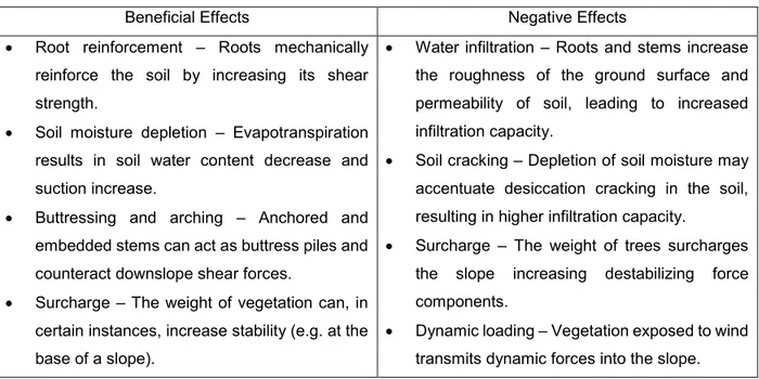
1.4 Vegetation effect on slope stability ... 19
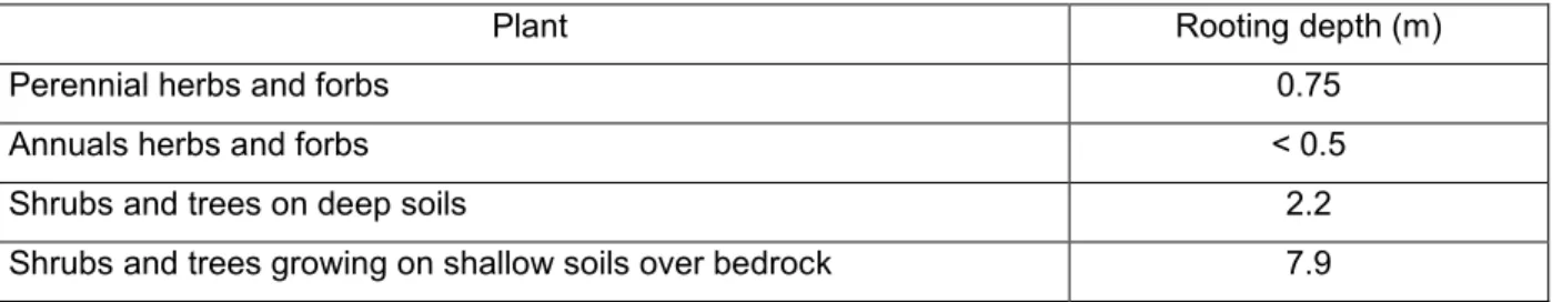
1.4.1 Root systems and root growth ... 21
1.4.2 Useful traits for reinforcing soil on slopes ... 22
x
1.4.3.1 Effect of roots on the soil hydraulic properties ... 23
1.4.3.2 Rainfall partition... 25
1.4.3.3 Effect of vegetation on the groundwater regime ... 26
1.4.4 Mechanical effect of vegetation on slope stability ... 27
1.4.4.1 Roots in a shallow landslide ... 27
1.4.4.2 Root failure modes ... 28
1.4.4.3 Root reinforcement ... 30
1.5 Objectives ... 33
Chapter 2 Test site overview... 37
2.1 Introduction ... 37
2.2 Stratigraphy ... 38
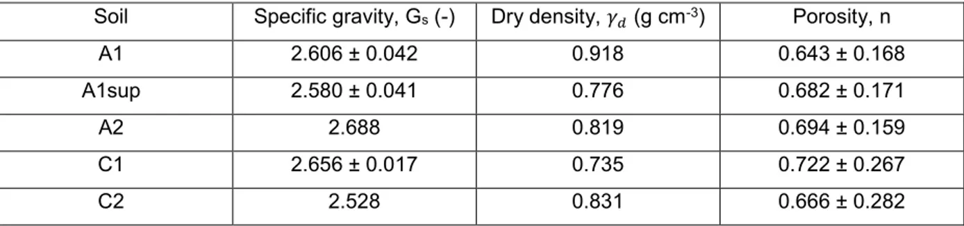
2.3 Soil physical properties ... 41
2.4 Slope topography ... 43
2.5 Vegetation and ground cover ... 44
Chapter 3 Hydraulic characterization of natural unsaturated pyroclastic soils ... 49
3.1 Introduction ... 49
3.2 Methods and materials ... 51
3.2.1 Void ratio of root-permeated soil ... 51
3.2.2 Hydraulic characterization ... 55
3.2.2.1 Saturated permeability ... 56
3.2.2.2 Wetting and drying cycles ... 58
3.2.2.3 High suction range ... 60
3.2.3 Dry biomass ... 61
3.2.4 Experimental data processing and filtering ... 61
3.2.4.1 Saturated permeability ... 61
3.2.4.2 Ku-pf apparatus data filter ... 62
3.2.5 Inverse analysis... 63
3.2.5.1 Objective function ... 63
xi
3.2.5.3 Main drying curve fitting ... 64
3.2.5.4 Hysteretic model calibration ... 68
3.2.6 Water capacity ... 71
3.3 Results and discussion ... 72
3.3.1 Saturated permeability ... 72
3.3.2 Drying and wetting cycles ... 73
3.3.3 High suction range ... 75
3.3.4 Inverse analysis... 76
3.3.4.1 Main drying curve fitting ... 76
3.3.4.2 Main wetting curve fitting ... 80
3.3.4.3 Sensitivity analysis of the hysteretic model ... 80
3.3.4.4 Assessment of the data sets size ... 81
3.3.4.5 Test replication and parameter dependency on porosity ... 83
3.3.5 Soil water capacity ... 89
3.3.6 Effect of roots on the soil hydraulic properties ... 90
3.4 Conclusions ... 93
Chapter 4 Groundwater regime interaction with atmosphere and vegetation ... 95
4.1 Introduction ... 95
4.2 Methods and materials ... 96
4.2.1 Test site characterization ... 96
4.2.2 Climate data ... 97
4.2.3 Meteorological data interpretation ... 99
4.2.3.1 Potential evapotranspiration ... 99
4.2.3.2 Evapotranspiration calculation parameters ... 102
4.2.3.3 Relative humidity estimation ... 103
4.2.4 Field instrumentation: TDR probes and tensiometers ... 103
4.2.5 Equipment calibration ... 107
4.2.5.1 Relation between dielectric constant and volumetric water content ... 107
xii
4.2.6 Root distribution ... 112
4.2.6.1 Roots sampling ... 112
4.2.6.2 Roots scanning and image analysis... 113
4.2.6.3 Root vertical distribution model ... 114
4.2.6.4 Root spatial distribution model ... 115
4.2.7 Water flow in the soil ... 116
4.2.8 Hydraulic response of the soil related to spatial root distribution ... 117
4.3 Results and discussion ... 117
4.3.1 Meteorological monitoring ... 117
4.3.1.1 Previous rainfall records in Moiano and Pimonte ... 117
4.3.1.2 Meteorological monitoring of Mount Faito ... 119
4.3.2 Considerations on vegetation and ground cover ... 126
4.3.3 Root distribution ... 127
4.3.3.1 Measurements of root density ... 127
4.3.3.2 Fitting of the root vertical distribution model ... 132
4.3.3.3 Fitting of the root lateral distribution model ... 134
4.3.4 Equipment calibration ... 137
4.3.4.1 Relation between dielectric constant and volumetric water content ... 137
4.3.4.2 Tensiometers ... 143
4.3.5 Monitored suction and volumetric water content ... 146
4.3.6 Comparison of field data and laboratory water retention curves ... 151
4.3.7 Groundwater vertical flow ... 155
4.3.8 Spatial distribution of water content and suction associated to root density ... 159
4.3.8.1 Fitting of the spatial distribution model to soil hydraulic behaviour observations ... 159
4.3.8.2 Relate root density indicators and soil hydraulic properties indicators ... 161
4.3.8.3 Considerations on the relations between root distribution and hydraulic propertied indicators 165 4.4 Conclusion ... 166
xiii
5.1 Introduction ... 168
5.2 Methods and materials ... 169
5.2.1 Soil strength considering the presence of roots ... 169
5.2.2 Soil hydro-mechanical characterization ... 169
5.2.2.1 Standard direct shear test ... 169
5.2.2.2 Direct shear test in unsaturated conditions ... 171
5.2.3 Quantification of the mechanical reinforcement of the soil by the roots ... 174
5.2.3.1 Root area ratio ... 175
5.2.3.2 Root tensile strength ... 175
5.2.3.3 Wu and Waldron model ... 176
5.2.3.4 Fibre bundle model... 178
5.2.4 Slope stability analysis ... 181
5.3 Results and discussion ... 181
5.3.1 Soil hydro-mechanical properties ... 181
5.3.1.1 Saturated conditions direct shear test ... 181
5.3.1.2 Unsaturated direct shear test ... 186
5.3.2 Mechanical reinforcement of the soil by the roots ... 190
5.3.3 Slope stability ... 191
5.3.3.1 Adopted parameters ... 191
5.3.3.2 Safety factor ... 192
5.3.3.3 Relative contribution of roots, suction and soil shear strength to the stability ... 197
5.4 Conclusion ... 200
Chapter 6 Conclusion and future work ... 202
6.1 Conclusion ... 202
6.2 Future work ... 203
References ... 206
Annexes ... 216 Annex A – List of boreholes for physical, hydraulic and mechanical characterization ... a Annex B – Species identified in Mount Faito ... c
xiv
Annex C – Data sampler for inverse analysis ... f Annex D – Saturated permeability ... r Annex E – Water content in the high suction range ... t Annex F – Fitting of the main drying from inverse analysis ... u Annex G – Fitting of the main wetting with inverse analysis ... y Annex H – Sensitivity analysis examples of the main wetting fitting parameters ... bb Annex I – Examples of simulations using fitting parameters of 1 and 2 cycles ... dd Annex J – Examples of simulations used for ku-pf apparatus test replication. ... ff Annex K – Root dry biomass in the ku-pf samples ... ii Annex L – WinRIZHO analysis procedure ... jj Annex M – Fitting of the vertical root distribution model procedure ... ll Annex N – Fitting of the spatial root distribution model procedure... nn Annex O – Tree survey: DBH and tree-to-vertical distance ... pp Annex P – Root vertical distribution raw characterization ... rr Annex Q – Vertical root distribution model fitting ... tt Annex R – Root lateral distribution model fitting ... vv Annex S – Monitored volumetric water content in Mount Faito ... kkk Annex T – Monitored suction ... ooo Annex U – Field suction and water content in the water retention plan ... sss Annex V – Spatial distribution of hydraulic observations ... uuu Annex W – Spatial distribution of hydraulic (model fitting) ... vvv Annex X – Fitting parameters of the spatial distribution model adapted to hydraulic observations ... kkkk Annex Y – Practical steps for the operation of the unsaturated direct shear testing equipment ... llll Annex Z – Calculation of root cohesion ... pppp Annex AA – Root cohesion calculated using different load distribution criteria in FBM ... tttt
xv
Index of figures
Figure 1 – Number of victims in the Campania region caused by landslides from 1580 to 1998 (Cascini et
al., 2008). ... 1
Figure 2 – Inventory map of the January 1997 landslides in the Sorrento Peninsula, (adapted from Calcaterra and Santo, 2004). ... 2
Figure 3 – Typical water retention curve (adapted from Vanapalli et al., 1999). ... 5
Figure 4 – Illustration of main and scanning water retention curves (adapted from Switala, 2016). ... 5
Figure 5 – Water retention curves of sandy, silty and clayey soils (Fredlund and Xing, 1994). ... 6
Figure 6 – Hysteretic loops in the water retention plan when saturation is (a) actual water saturation and (b) apparent water saturation. ... 8
Figure 7 – Scheme of the events and conditions that lead to landslides in pyroclastic soil covers. ... 11
Figure 8 – Scheme of the main morphology associated to debris flow type of landslide (Di Crescenzo and Santo, 2005). ... 12
Figure 9 – Grain size distribution of the soils present at Monteforte Irpino test site (adapted from Pirone et al., 2015b). ... 13
Figure 10 – Evolution of the matric suction with time in different soil layers (Pirone et al., 2015a). ... 14
Figure 11 – Monitoring data of a test site in Cervinara (adapted from Urciuoli et al., 2016). ... 15
Figure 12 – Evolution of matric suction and degree of saturation with depth for different instants during the wet season in Monteforte Irpino (adapted from Urciuoli et al., 2016). ... 16
Figure 13 – Hourly measurements of total head during a rainfall even in the test site at Cervinara (adapted from Urciuoli et al., 2016). ... 16
Figure 14 – Main drying WRCs and HPFs (Nicotera et al., 2010). ... 17
Figure 15 – Comparison of the main drying WRC and the field measurements of Monteforte Irpino (Pirone et al., 2014). ... 18
Figure 16 – Results of the saturated triaxial tests (Papa et al., 2008), in which f’ represents the critical friction angle. ... 18
Figure 17 – Vegetation-slope interactions (Wilkinson et al., 2002). ... 19
Figure 18 – Different types of root systems (adapted from Switala, 2016). ... 22
Figure 19 – Changes in infiltration rate under alfalfa culture with time (in Angers and Caron, 1998). ... 24
Figure 20 – Drying (a) and wetting (b) branch of the water retention loop of bare soil (B) and vegetated soil with increasing distance between seedlings (60, 120 and 180 mm) presented in Ng et al. (2016b). ... 25
Figure 21 – Weight of each component contributing to the slope stability of different vegetation covers and cultivations in comparison to fallow soil (red line) by Kim et al. (2017). ... 27
Figure 22 – Solicitation of the root reinforcement at different locations along the sliding surface of a shallow landslide: (a) tension, (b) shear and (c) compression (Dias et al., 2017). ... 28
xvi
Figure 24 – Measured critical load compared with the theoretical solutions (adapted from Wu et al., 1988).
... 30
Figure 25 – Scheme of the stresses in the root during shear (Dias et al., 2017a). ... 32
Figure 26 – Comparison of the root-permeated soil reinforcement as a function of displacement of FBM and W&W models (Schwarz et al., 2010). ... 32
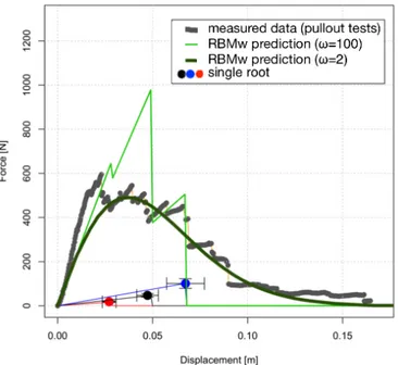
Figure 27 – Measured and simulated force-displacement behaviour of a bundle of roots (adapted from Schwarz et al., 2013). ... 33
Figure 28 – Soil aggregates and pumices hanging from roots in a cultivated area near Sarno (Campania, Italy). ... 34
Figure 29 – Macropores created by roots (Ghestem et al., 2011). ... 35
Figure 30 – Roots that failed by pull out in a previous landslide in the region of Campania. ... 36
Figure 31 – Test site location on satellite images (source: Google Earth). ... 37
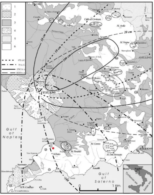
Figure 32 – Areas of pyroclastic deposition of several eruptions of Vesuvius volcano (adapted from Di Crescenzo and Santo, 2005). Approximate location of Mount Faito test site. ... 38
Figure 33 – Boreholes performed in Mount Faito test site and their spatial distribution. ... 40
Figure 34 – Mean soil stratigraphoc profile present at Mount Faito and soil classification according to the USCS. ... 41
Figure 35 – Grain size distribution of Mount Faito Faito soils. ... 42
Figure 36 – Projected longitudinal profile of cell 1 and 2. ... 44
Figure 37 – Photograph of the site on February 17th, 2017. ... 44
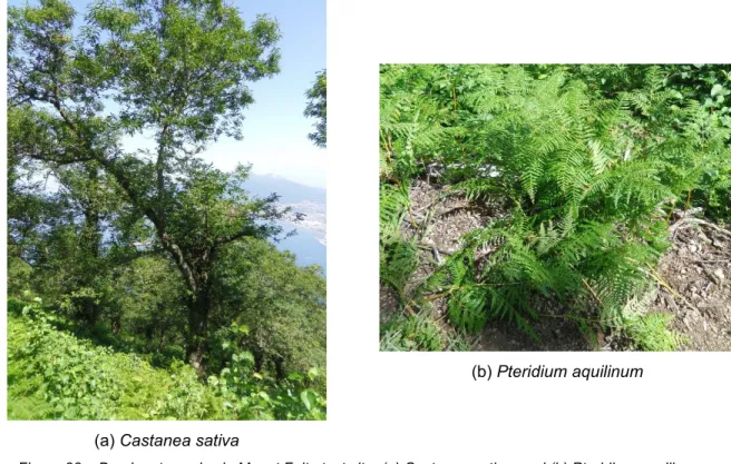
Figure 38 – Dominant species in Mount Faito test site: (a) Castanea sativa, and (b) Pteridium aquilinum. ... 45
Figure 39 – Photos of cell 1 from March to October 2017. ... 46
Figure 40 – Photos of cell 1 from November 2018 to April 2018. ... 47
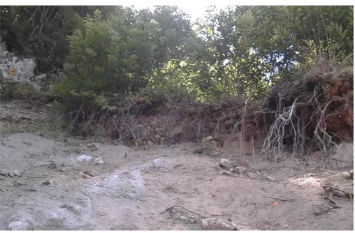
Figure 41 – Soil erosion exposing roots. ... 48
Figure 42 – Formation of a frozen soil layer. ... 48
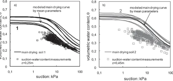
Figure 43 – Comparison of laboratory main drying curves and field measurements (adapted from Papa et al., 2013). ... 50
Figure 44 – Variation of the roots of Castanea sativa specific gravity with depth in Mount Faito: individual measurements and mean and respective standard deviation. ... 52
Figure 45 – Specific gravity of the Castanea sativa roots for different diameter classes. ... 53
Figure 46 – Scheme of the test sequence and summarized description. ... 55
Figure 47 – Soil sample extrusion from the borehole. ... 55
Figure 48 – Soil sample after extrusion. ... 55
Figure 49 – Setup used to determine the saturated permeability at constant head. ... 56
Figure 50 – Scheme of the setup to determine the saturated permeability and indication of basic operation instructions. ... 56
xvii
Figure 51 – Permeameter: soil mould and upper and bottom supports. ... 57
Figure 52 – ku-pf apparatus used in the experimentation. ... 58
Figure 53 – Sample support on the scale of the ku-pf apparatus. ... 58
Figure 54 – Scheme of the sample support (adapted from Nicotera et al., 2010). ... 58
Figure 55 – Tensiometer (do not hold the tensiometer in this manner during the saturation). ... 59
Figure 56 – Setup of the saturation of tensiometers. ... 59
Figure 57 – Setup for the calibration of the tensiometers. ... 59
Figure 58 – ku-pf software on the calibration of tensiometers. ... 59
Figure 59 – Support with guides to make holes in the sample to insert the tensiometers. ... 60
Figure 60 – Equipment used to make the holes for the tensiometers. ... 60
Figure 61 – Full pressure plate system. ... 61
Figure 62 – Position of the samples inside the pressure plate chamber. ... 61
Figure 63 – Measurements of a single test presented as an example of the water flow through the sample with time, where the slope of the linear regression is equal to the saturated permeability of the soil. ... 62
Figure 64 – Soil profile and identified observation points. ... 67
Figure 65 – Interface for the definition of the initial conditions in terms of suction head of HYDRUS-1D. . 67
Figure 66 – Comparison of the water capacity resultant from two different water retention curves with different AEV (Fredlund & Rahardjo, 2012). ... 72
Figure 67 – Comparison of mean saturated permeability and mean porosity of different soil layers with depth. ... 73
Figure 68 – Monitored suction at bottom and top tensiometers and wet soil weight of the sample 1.4.1 (soil A2) by the ku-pf apparatus. ... 74
Figure 69 – Suction at the bottom and top tensiometer, vertical gradient and wet soil weight of a single wetting step monitored at the ku-pf apparatus of sample 1.7.2 (soil A1). ... 75
Figure 70 – Experimental drying-wetting loops obtained for sample 1.7.2 (soil A1), in terms of volumetric water content (vwc). ... 75
Figure 71 – Main drying WRC of sample 1.7.2 (soil A1) with the objective function data sets. ... 76
Figure 72 – HPF of the main drying of sample 1.7.2 (soil A1) with the measured saturated permeability. 76 Figure 73 – Mean main drying WRC obtained from inverse analysis. ... 77
Figure 74 – Mean main drying HPF obtained from inverse analysis. ... 77
Figure 75 – Representation of the mean and standard deviation of the fitting parameters of the main drying curve for each soil type. ... 78
Figure 76 – Sensitivity analysis of the fitting parameters of the main drying performed on sample 1.7.2 (soil A1). ... 79
Figure 77 – Main loop of the WRC with the experimental measurements of sample 1.7.2 (soil A1). ... 80
Figure 78 – Sensitivity analysis of the fitting parameters of the main wetting performed on sample 1.7.2 (soil A1). ... 81
xviii
Figure 79 – Simulation of the full test using the fitting parameters from 1 cycle (left side) and 2 cycles (right
side) and comparison with the experimental data... 82
Figure 80 – Comparison of the fitted parameters of the main wetting curve using 1 or 2 cycles. ... 83
Figure 81 – Main wetting branch fitting parameters comparison with soil porosity per soil type. ... 84
Figure 82 – Relationship between the parameters 𝛼𝑑 and 𝛼𝑖 per soil type and respective standard deviation. ... 85
Figure 83 – Relationship between 𝜃𝑠𝑑 and 𝜃𝑠𝑖 and soil porosity of the tested samples. ... 85
Figure 84 – Simulation of drying-wetting cycles of sample 1.7.2 with the fitting parameters of sample 1.9.2 (soil A1). ... 87
Figure 85 – Differences between suction estimations of the best fitting (case 4) and the fitting cases 1, 2 and 3. ... 88
Figure 86 – Water capacity and hydraulic permeability function of each soil type computed with the mean fitting parameters of the main (a) drying and (b) wetting branch. ... 89
Figure 87 – Mean and standard deviation of the maximum water capacity (Cmax) of each soil type. ... 90
Figure 88 – Saturated permeability, soil porosity and root dry biomass in each soil layer with depth per soil layer. ... 91
Figure 89 – Main water retention loop of soil (a) A1 and (b) A1sup. ... 92
Figure 90 – Water capacity (C) of the main wetting curves of soil A1 and A1sup. ... 92
Figure 91 – Location of the meteorological stations (Google Earth image). ... 97
Figure 92 – Meteorological station at Mount Faito test site. ... 98
Figure 93 – Extra-terrestrial radiation along the year for Mount Faito. ... 103
Figure 94 – Instrumented area: trees location (red numbered circles) relative to the profiles’ location (identified by letters) grouped in cell 1 and cell 2. ... 104
Figure 95 – Location of the instrumentation in each profile. ... 105
Figure 96 – The soil is being removed from the tube and identified with the help of a geologist. ... 106
Figure 97 – The tube is being pushed into the soil using a hammer. ... 106
Figure 98 – Interior and exterior cooper tubes to install tensiometers. ... 106
Figure 99 – Tube and extension used to open a borehole for the installation of TDR probes. ... 106
Figure 100 – Vacuum dial gauge and digital measurement adaptor installed on a Jet Fill tensiometer sided with a tradition SDEC France tensiometer. ... 107
Figure 101 – TDR probe dimensions. ... 109
Figure 102 – Plexiglas base glued to the mould. ... 110
Figure 103 – Cap, weight and latex disc. ... 110
Figure 104 – Pressure regulator and vacuum dial gauge. ... 110
Figure 105 – Vacuum converter. ... 110
Figure 106 – Equipment used to read the dielectric constant (computer, battery, TDR100 and cables). 110 Figure 107 – SDEC France tensiometers with different initial air columns. ... 111
xix
Figure 108 – Borehole extrusion (a), sectioning (b) and root washing (c). ... 112
Figure 109 – Bag storing roots in alcohol 15%. ... 112
Figure 110 – Procedure to scan roots: (a) root washing in a sieve, (b) spreading of roots on the glass board with a film of water, and (c) roots drying with absorbent paper. ... 113
Figure 111 – Example of a scanned roots image. ... 113
Figure 112 – Shadows created by the water meniscus. ... 114
Figure 113 – Root before (a) and after (b) erasing the mycorrhizas... 114
Figure 114 – Total rainfall cumulated along each year in Pimonte and Moiano meteorological stations. 118 Figure 115 – Maximum daily rainfall recorded in each year in Pimonte and Moiano meteorological stations. ... 118
Figure 116 – Mean and standard error of the monthly rainfall in Pimonte and Moiano meteorological stations. ... 118
Figure 117 – Daily rainfall registered by the meteorological stations at Moiano, Pimonte and Mount Mount Faito. ... 119
Figure 118 – Comparison of the daily rainfall recorded in Moiano and Pimonte with Mount Faito. ... 119
Figure 119 – Daily rainfall at Mount Faito from January 2017 to September 2018. ... 120
Figure 120 – Mean and standard error of the monthly rainfall of Moiano and Pimonte meteorological stations and the monthly rainfall recorded in Mount Faito. ... 120
Figure 121 – Small landslide on the side of the road that leads to the study site... 121
Figure 122 – Maximum, mean and minimum temperature recorded in Moiano and Mount Faito along the year. ... 122
Figure 123 – Comparison of the Maximum, mean and minimum temperature recorded in Moiano and Mount Faito. ... 122
Figure 124 – Maximum, mean and minimum temperature at Mount Faito from January 2017 to September 2018. ... 123
Figure 125 – Comparison of the measured and calculated relative humidity (RH). ... 123
Figure 126 – Relative humidity (RH) in Mount Faito from September 2017 to September 2018. ... 124
Figure 127 – Recorded maximum, mean and minimum daily relative humidity at Mount Faito. ... 124
Figure 128 – Recorded mean wind velocity at Mount Faito. ... 125
Figure 129 – Recorded mean soil temperature at the depths of 0. 2m and 0.5 m at Mount Faito. ... 125
Figure 130 – Recorded net radiation at Mount Faito. ... 125
Figure 131 – Reference evapotranspiration (ET0) calculated with the meteorological data of Mount Faito. ... 126
Figure 132 – Comparison of two methods of calculating reference evapotranspiration (ET0). ... 126
Figure 133 – Location of the soil profiles (identified with letters) in the polygons and trees (identified with numbers). ... 127
xx
Figure 134 – Increase in cumulative root dry biomass relative to the total root biomass with depth for all soil cores. ... 128 Figure 135 – Dry roots biomass measured in profiles NT and T per unit volume of soil. ... 128 Figure 136 – Example of grouped root characteristics in four diameter classes for a typical soil core (1S). ... 129 Figure 137 – Mean and standard error of the root length per unit soil volume for four diameter classes with depth. ... 130 Figure 138 – Mean and standard error of the root volume per unit soil volume for four diameter classes with depth. ... 130 Figure 139 – Mean and standard error of the number of root tips per unit soil volume for four diameter classes with depth. ... 130 Figure 140 – Mean and standard error of the root dry biomass per unit soil volume with depth. ... 130 Figure 141 – Relation between root dry biomass and the mean (a) root length, (b) number of root tips, and (c) root volume per unit volume of soil, and (d) the relation between root length and number of root tips. ... 131 Figure 142 – Cumulative relative (a) root length, (b) root volume, (c) number of root tips, and (d) root biomass with depth given by the fitted β-model. ... 133 Figure 143 – Spatial root distribution fitting to the root density in terms of biomass (0.25<z<0.5 m). ... 135 Figure 144 – Determination coefficient (R2) of the root lateral distribution for different root density indicators. ... 136 Figure 145 – Comparison of the grain size distribution of the soil of Mount Faito (A1, A2, C1) and Monteforte (1, 2, 6) (adapted from Dias et al., 2018). ... 138 Figure 146 – Soil dielectric constant and respective volumetric water content (vwc) along the wetting and drying phases of each tested soil. ... 139 Figure 147 – Comparison of the dielectric constants and volumetric water content (vwc) of all tested soils to the universal equations (Topp and Ledie)... 140 Figure 148 – Comparison of the models fitted to Mount Faito data and Monteforte to the experimental data. ... 142 Figure 149 – Comparison between the experimental data of soil B and the soil studied by Papa and Nicotera (2012). ... 143 Figure 150 – Scheme of the setup and reference water pressures. ... 144 Figure 151 – Relation between digital measurement and the real pressure. ... 144 Figure 152 – Evolution of the suction (s) along time for different initial air columns... 145 Figure 153 – Evolution of the air column along time for different initial air columns... 145 Figure 154 – Daily rainfall (a) and mean and standard deviation of the volumetric water content (vwc) measured in cells 1 and 2 in soil A1 and A2 (b), soil B (c) and soil C1 and C2 (d). ... 147
xxi
Figure 155 – Volumetric water content (vwc) in the profiles NT and T comparison with the mean values in soil A1 and A2. ... 148 Figure 156 – Average and standard deviation of the suction (s) in cells 1 and 2 in comparison with the rainfall. ... 149 Figure 157 – Monitored suction (s) in profiles T and NT in comparison with the mean suction in soil A1 and A2. ... 150 Figure 158 – Comparison of the mean water content (vwc) and suction (s) measured in situ and the envelope of the main loop obtained in the laboratory. ... 152 Figure 159 – Mean field measurements of suction (s) and volumetric water content (vwc) of soils A and C. ... 153 Figure 160 – Measurements in profiles NT and T of suction (s) and volumetric water content (vwc). ... 154 Figure 161 – Comparison between field measurements of suction (s) and volumetric water content (vwc) in profiles T and NT and WRC envelops. ... 154 Figure 162 – Mean hydraulic head (h) for cells 1 and 2 per soil layer. ... 156 Figure 163 – Mean vertical gradient in couples of measurements in comparison with rainfall and reference evapotranspiration (ET0). ... 157 Figure 164 – Mean suction (s) and volumetric water content (vwc) along the soil profile before and after the rainfall events of September 2017. ... 158 Figure 165 – Vertical gradient in profiles T and NT in comparison to rainfall and reference evapotranspiration (ET0). ... 159 Figure 166 – Coefficient of determination (R2) of different hydraulic observations in soil A1 and A2 to fit the spatial distribution model for a maximum tree-to-profile distance of (a) 10 m, (b) 8 m, and (c) considering only the nearest tree to the profile. ... 160 Figure 167 – Competition index for each profile fitted for the data of (a) root biomass, and (b) vertical distribution of the number of root tips. ... 162 Figure 168 – Coefficient of determination (R2) for each hydraulic properties’ indicator fixing the competition index of the root density in terms of biomass. ... 163 Figure 169 – Minimum volumetric water content (min vwc), minimum vertical gradient and root biomass for the same competition indexes considering all the trees in a range of up to 10 m from the soil profiles. . 163 Figure 170 – Coefficient of determination (R2) for each hydraulic properties’ indicator fixing the competition index of the vertical root distribution parameter (β-value) in terms of root tips. ... 164 Figure 171 – Minimum suction and β-values (number of root tips) for the same competition indexes considering all the trees in a range of up to 8 m from the profiles. ... 164 Figure 172 – Insert soil sample in the shear box. ... 170 Figure 173 – Traditional direct shear test equipment (Esposito, 2017). ... 170 Figure 174 – Shear box (adapted from Evangelista et al., 2004). ... 171
xxii
Figure 175 – Unsaturated conditions direct shear testing equipment (adapted from Evangelista et al., 2004): A represents the top view and B the transversal view. ... 172 Figure 176 - Scheme of pressure regulation circuits and transducers used in the suction-controlled direct shear test (adapted from Papa and Nicotera, 2011). ... 173 Figure 177 – Assemblage of the unsaturated direct shear test in unsaturated: (a) lower the water level and moist the porous stone; (b) place the lower ring with screws and position the metallic strips; (c) position the upper part and connect it to the loading cell; (d) push the soil sample into the box using an extruder; and (e) position the upper porous stone and the sphere. ... 174 Figure 178 – Tensile strength relation with diameter of different species (Bischetti et al., 2009). ... 176 Figure 179 – Scheme of the response of the roots with different orientations with the shear zone. ... 178 Figure 180 – Flowchart for the FBM computation. ... 179 Figure 181 – Vertical displacements (δv) during the consolidation phase in samples of soil A1. ... 183 Figure 182 – Vertical displacements (dv) during the saturation phase in samples of soil A1. ... 183 Figure 183 – Ratio between shear and confining stress (τ/σ’), and vertical displacement (dv) measured during the shear phase with horizontal displacement (dh) in samples of soil A1. ... 184 Figure 184 – Ratio between shear and confining stress (τ/σ’), and vertical displacement (dv) measured with horizontal displacement (dh) during the shear phase of NC and OC samples of soil C1. ... 185 Figure 185 – Limit shear strength and Mohr-Coulomb failure envelope of soil (a) A1 and (b) C1: confining stress (σ’v) and correspondent shear strength (τ). ... 185 Figure 186 – Measurement of suction (s) after applying the chamber air pressure. ... 186 Figure 187 – Initial (a) void ratio (e) and (b) volumetric water content (vwc) for each measured suction (s) (the mean WRCs from Chapter 3 and an additional point correspondent to saturation). ... 187 Figure 188 – Vertical settlement (dv) during consolidation. ... 187 Figure 189 – Shear stress (τ) and vertical displacement (dv) with horizontal displacement (dh) during the shear phase. ... 188 Figure 190 – Ratio between shear and Bishop stress (t/s’), and vertical displacement (dv) measured with horizontal displacement (dh) during the shear phase. ... 189 Figure 191 – Limit shear strength (τ) and Mohr-Coulomb failure envelopes of soil C1 obtained from direct shear tests in saturated (sat) and unsaturated (unsat) conditions. ... 189 Figure 192 – Mean root cohesion obtained from W&W model when k’’=1 (W&W0) and when k’’=0.56 (W&W) after Bischetti et al. (2009) and FBM with load distribution according with the number of roots, the roots diameter and the roots area class (referred as number, diameter, and area, respectively) with depth. .. 190 Figure 193 – Safety factor (SF) along the monitoring period (a) assuming failure surfaces at different depths and (b) a close up in the most critical depths (2.2 m, 2.5 m and 2.7 m). ... 192 Figure 194 – Variation of the safety factor (SF) with increasing depth of the failure surface in soil A1 and A2. ... 193
xxiii
Figure 195 – Sliding surfaces and geological profiles in the sliding zone of previous landslides (adapted from Di Crescenzo and Santo, 1999). ... 194 Figure 196 – Safety factor (SF) ignoring the root contribution assuming failure surfaces at different depths (a) and a zoom of the lower range of SF (b). ... 195 Figure 197 – Safety factor over time assuming a failure surface in different soil layers in the profile of Monteforte Irpino (adapted from Pirone et al., 2015b). ... 196 Figure 198 – Minimum estimated safety factor (SF) for different slope angles considering and not the presence of roots. ... 197 Figure 199 – Contribution of the soil, roots and suction to the safety factor (SF) in soil (a) A1(z=0.2 m) and (b) A2 (z=0.5 m), and (c) A2 (z=0.9 m) ... 198 Figure 200 – Contribution of the soil, roots and suction to the safety factor (SF) in soil C1 and C2. ... 199 Figure 201 – Excel worksheet SSA to with ku-pf monitoring data to be used as source. ... f Figure 202 – Output worksheet HYDRUS# containing the sampled boundary conditions (INPUT 1), the data sets (INPUT 2), data set size and time information on the top right corner, initial estimation of the input parameters right bellow, and the initial conditions at the bottom right. ... g Figure 203 – Output worksheet ‘hysteresis’ containing the sampled boundary conditions (columns A to D), the data sets (columns F to P), data set size and time information on the top right corner, initial estimation of the input parameters right bellow, the initial conditions, and the fitted parameters of the main drying curve. ... h Figure 204 – Probability density function of the saturated permeability of soil A1sup, A1, A2 and C1. ... s Figure 205 – Main drying WRC of each soil type (a-e) and comparison among their mean (f) obtained from inverse analysis. ... w Figure 206 – Main drying HPF of each soil type (a-e) and comparison among their mean (f) obtained from inverse analysis. ... x Figure 207 – Examples of main drying-wetting loops of different soil types. ... z Figure 208 – Sensitivity analysis of the fitting parameters of the main wetting performed on sample N1 (soil A1sup). ... bb Figure 209 – Sensitivity analysis of the fitting parameters of the main wetting performed on sample 1.4.1 (soil A2). ... bb Figure 210 – Sensitivity analysis of the fitting parameters of the main wetting performed on sample 2.12.2 (soil C1). ... cc Figure 211 – Simulation of the full test using the fitting parameters from 1 cycle (left side) and 2 cycles (right side) and comparison with the experimental data of sample 1.7.2 (soil A1). ... dd Figure 212 – Simulation of the full test using the fitting parameters from 1 cycle (left side) and 2 cycles (right side) and comparison with the experimental data of sample 1.4.1 (soil A2). ... dd Figure 213 – Simulation of the full test using the fitting parameters from 1 cycle (left side) and 2 cycles (right side) and comparison with the experimental data of sample 2.12.2 (soil C1). ... ee
xxiv
Figure 214 – Simulation of the full test using the fitting parameters from 1 cycle (left side) and 2 cycles (right side) and comparison with the experimental data of sample 1.1 (soil C2). ... ee Figure 215 – Simulation of the drying and wetting cycles of sample N2 with the fitting parameters of sample N1 (soil A1sup). ... ff Figure 216 – Simulation of the drying and wetting cycles of sample 1.4.1 with the fitting parameters of sample 1.2.1 (soil A2). ... gg Figure 217 – Simulation of the drying and wetting cycles of sample 2.13.1 with the fitting parameters of sample 2.12.2 (soil C1). ... hh Figure 218 – Sequence of steps followed in the image analysis. ... kk Figure 219 – Root density in terms of root dry biomass per unit volume of soil with depth. ... rr Figure 220 – Cumulative root density in terms of root dry biomass per unit volume of soil with depth. ... rr Figure 221 – Total root length per unit soil volume with depth in cell 1 (a) and cell 2 (b). ... rr Figure 222 – Total root volume per unit soil volume with depth in cell 1 (a) and cell 2 (b). ... ss Figure 223 – Total number of root tips per unit soil volume with depth in cell 1 (a) and cell 2 (b). ... ss Figure 224 –Estimation of root length for verticals with different competition indexes (dmax = 10 m). ... ww Figure 225 –Estimation of root length for verticals with different competition indexes (dmax = 8 m). ... xx Figure 226 –Estimation of root length for verticals with different competition indexes (dmin ). ... yy Figure 227 – Estimation of number of root tips for verticals with different competition indexes (dmax = 10 m). ... zz Figure 228 – Estimation of number of root tips for verticals with different competition indexes (dmax = 8 m). ... aaa Figure 229 – Estimation of number of root tips for verticals with different competition indexes (dmin). ... bbb Figure 230 – Estimation of beta-values for verticals with different competition indexes (d = 10 m, all trees) ... ccc Figure 231 – Estimation of beta-values for verticals with different competition indexes (d = 10 m, uphill) ... ddd Figure 232 – Estimation of beta-values for verticals with different competition indexes (d = 10 m, downhill) ... eee Figure 233 – Estimation of beta-values for verticals with different competition indexes (d = 8 m, all trees). ... fff Figure 234 – Estimation of beta-values for verticals with different competition indexes (d = 8 m, uphill). ggg Figure 235 – Estimation of beta-values for verticals with different competition indexes (d = 8 m, downhill). ... hhh Figure 236 – Estimation of beta-values for verticals with different competition indexes (d = dmin). ... iii Figure 237 – Monitored volumetric water content (vwc) in cell 1 in soil A1 and A2 at Mount Faito. ... kkk Figure 238 – Monitored volumetric water content (vwc) in cell 1 in soil B, C1 and C2 at Mount Faito. ... lll Figure 239 – Monitored volumetric water content (vwc) in cell 2 in soil A1 and A2 at Mount Faito. ... mmm
xxv
Figure 240 – Monitored volumetric water content (vwc) in cell 2 in soil B, C1 and C2 at Mount Faito. .... nnn Figure 241 – Monitored suction (s) in cell 1 in soil A1 and A2. ... ooo Figure 242 – Monitored suction (s) in cell 1 in soil C1 and C2. ... ppp Figure 243 – Monitored suction (s) in cell 2 in soil A1 and A2. ... qqq Figure 244 – Monitored suction (s) in cell 2 in soil C1 and C2. ... rrr Figure 245 – Field measurements in cell 1 of volumetric water content (vwc) and suction (s). ... sss Figure 246 – Field measurements in cell 2 of volumetric water content (vwc) and suction (s). ... ttt Figure 247 – Spatial distribution of the hydraulic gradient considering the effect of all the trees in a range of 8 m from the verticals. ... vvv Figure 248 – Spatial distribution of suction in soil A1 considering the effect of all the trees in a range of 8 m from the verticals. ... www Figure 249 – Spatial distribution of suction in soil A2 considering the effect of all the trees in a range of 8 m from the verticals. ... xxx Figure 250 – Spatial distribution of the volumetric water content in soil A1 considering the effect of all the trees in a range of 8 m from the verticals. ... yyy Figure 251 – Spatial distribution of the volumetric water content in soil A2 considering the effect of all the trees in a range of 8 m from the verticals. ... zzz Figure 252 – Spatial distribution of the hydraulic gradient considering the effect of all the trees in a range of 10 m from the verticals. ... aaaa Figure 253 – Spatial distribution of suction in soil A1 considering the effect of all the trees in a range of 10 m from the verticals. ... bbbb Figure 254 – Spatial distribution of suction in soil A2 considering the effect of all the trees in a range of 10 m from the verticals. ... cccc Figure 255 – Spatial distribution of the volumetric water content in soil A1 considering the effect of all the trees in a range of 10 m from the verticals. ... dddd Figure 256 – Spatial distribution of the volumetric water content in soil A2 considering the effect of all the trees in a range of 10 m from the verticals. ... eeee Figure 257 – Spatial distribution of the hydraulic gradient considering the effect of the closest tree from the vertical. ... ffff Figure 258 – Spatial distribution of suction in soil A1 considering the effect of the closest tree from the vertical. ... gggg Figure 259 – Spatial distribution of suction in soil A2 considering the effect of the closest tree from the vertical. ... hhhh Figure 260 – Spatial distribution of the volumetric water content in soil A1 considering the effect of the closest tree from the vertical. ... iiii Figure 261 – Spatial distribution of the volumetric water content in soil A2 considering the effect of the closest tree from the vertical. ... jjjj
xxvi
Figure 262 – Root cohesion per vertical with depth FBM (load distributed according to the root cross-section area). ... tttt Figure 263 – Root cohesion per vertical with depth FBM (load distributed according to the root diameter). ... tttt Figure 264 – Root cohesion per vertical with depth FBM (equally distributed load by all roots). ... uuuu
xxvii
Index of tables
Table 1 – Common classification of landslides occurring in shallow pyroclastic soil covers according to the updated Varnes classification proposed by Hungr et al. (2014). ... 12 Table 2 – Beneficial and negative effects of vegetation on slope stability (Gray and Sotir, 1996). ... 20 Table 3 – Rooting depth of different types of plants and soil layer thicknesses (Stokes et al., 2009)... 21 Table 4 – Lateral root growth in terms of radius for different plants (Stokes et al., 2009). ... 21 Table 5 – Summarized desirable root traits to be considered in the slope stability analysis (Stokes et al., 2009). ... 23 Table 6 – Detailed description of the geological profile at Mount Faito. ... 39 Table 7 – Thickness of each soil layer found in the boreholes represented in Figure 33. ... 40 Table 8 – Liquid limit, plastic limit, and plasticity index of soil C1 and C2 collected at Mount Faito performed by Mastantuono (personal communication). ... 43 Table 9 – Mean and standard deviation of soil physical properties: specific gravity (Gs), dry density (𝛾𝑑) and soil porosity. ... 43 Table 10 – Summary of the specific gravity (dimensionless) of the root wood to be adopted in the calculation of root volume for each experiment and respective soil and root conditions. ... 54 Table 11 – Scheme of the input table of the initial estimation of the fitting parameters of the main drying curve in HYDRUS-1D (an example). ... 66 Table 12 – Scheme of the input table of the boundary conditions for the main drying curve fitting in HYDRUS-1D. ... 66 Table 13 – Scheme of the input table of the data sets for the main drying curve fitting in HYDRUS-1D. .. 67 Table 14 – Scheme of the input table of the initial estimation of the fitting parameters of the main wetting curve in HYDRUS-1D (an example). ... 70 Table 15 – Scheme of the input table of the boundary conditions for the main wetting curve fitting in HYDRUS-1D. ... 70 Table 16 – Scheme of the input table of the data sets for the main drying curve fitting in HYDRUS-1D. .. 70 Table 17 – Mean and standard deviation of log(Ksat) of each soil type... 72 Table 18 – Coefficient of determination of the logarithm of suction along time in the fitting of 1 or 2 cycles (drying-wetting loops). ... 83 Table 19 – Fitted parameters adopted from the sample ‘Fit’ and ‘Simulate’ for each of the cases (1 to 4). ... 86 Table 20 – Location of the meteorological stations. ... 98 Table 21 – Time resolution of data recording and working period in each meteorological station. ... 99 Table 22 – Constants necessary for the calculation of the psychometric constant. ... 100 Table 23 – List of constants used in the calculation of the reference evapotranspiration. ... 102 Table 24 – Instrumentation depths of TDR probes and tensiometers in profiles... 105
xxviii
Table 25 – Input parameters to PC-TDR. ... 109 Table 26 – Objectives of the calibration tests of the tensiometers. ... 111 Table 27 – Root density indicators (D is root diameter). ... 115 Table 28 – Selected hydraulic property indicators for the fitting of the spatial distribution model. ... 117 Table 29 – Parameter 𝛽 obtained per soil profile. ... 132 Table 30 – Recommended spatial root distribution models. ... 137 Table 31 – Mean soil physical properties of Mount Faito (A1, A2 and C1) and of Monteforte (1, 2 and 6 in Pirone et al., 2015a) (adapted from Dias et al.,2018). ... 137 Table 32 – Properties of the tested samples (adapted from Dias et al.,2018). ... 138 Table 33 – Calibration parameters of the polynomial model. ... 140 Table 34 – Calibration parameters of the logarithmic model. ... 141 Table 35 – Calibration parameters of the Roth model. ... 141 Table 36 – Initial air column of the tests. ... 145 Table 37 – Vertical settlements (dv) and void ratio (e) change along the tests on soil A1. ... 182 Table 38 – Vertical settlements (dv) and void ratio (e) change along the tests on soil C1 in saturated conditions. ... 182 Table 39 – Settlements (dv) and void ratio (e) change along the tests on soil C1 in unsaturated conditions. ... 186 Table 40 – Adopted soil properties in the calculation of slope stability. ... 191 Table 41 – Date, trench, soil type and depth of each borehole collected at Mount Faito for physical and hydraulic characterization. ... a Table 42 – List of samples collected in Mount Faito for mechanical characterization. ... b Table 43 – List of identified species in July and September 2017 at Mount Faito test site (Annalisa Santangelo and Sandro Strumia, personal communication). ... c Table 44 – Saturated permeability of individual tests and average value per sample... r Table 45 – Saturated permeability of several samples performed by Mastantuono (personal communication). ... s Table 46 – Measured and adopted values of volumetric water content (vwc) and suction for the objective function (inverse analysis) in the high suction range. ... t Table 47 – Fitted parameters of the main drying WRC and HPF of each sample and respective R2-index of the fitting. ... u Table 48 – Mean fitted parameters of the main drying WRC and HPF of each soil type. ... u Table 49 – Standard deviation of the fitted parameters of the main drying WRC and HPF of each soil type. ... v Table 50 – Fitted parameters of the main wetting WRC and HPF of each sample and respective R2-index of the fitting using data from 1 cycle, as well as the saturated hydraulic conductivity adopted in the model. ... y
xxix
Table 51 – Mean fitted parameters of the main wetting WRC and HPF of each soil type. ... aa Table 52 – Standard deviation of the fitted parameters of the main wetting WRC and HPF of each soil type. ... aa Table 53 – Roots dry biomass collected in the samples tested in the permeameter and/or the ku-pf apparatus. ... ii Table 54 – Diameter at breast height (DBH) and tree to profile distance. ... pp Table 55 – Tree position relatively to a profile (1 – uphill, 2 – downhill). ... qq Table 56 – 𝛽-value from the calibration of the exponential model (D stands for root diameter in mm). ... tt Table 57 – R2-index relative to the fitting of the 𝛽-value (D stands for root diameter in mm). ... uu Table 58 – Observed root density indicators (D stands for root diameter in mm). ... vv Table 59 – Fitting parameters of the spatial root distribution model for each root density indicator and each tree position and distance tree-to-vertical range. ... jjj Table 60 – Observed parameters for the fitting of the spatial distribution model. ... uuu Table 61 – Constants added to the hydraulic observations of gradient. ... uuu Table 62 – Fitting parameters of the spatial distribution model adapted to hydraulic observations. ... kkkk Table 63 – Mean root cohesion with depth using different models in MPa. ... uuuu Table 64 – Standard deviation of the root cohesion with depth using different models in MPa. ... vvvv Table 65 – Coefficient k’’ variation with depth for each load distribution criteria of FBM. ... vvvv
xxx
List of symbols
Greek letters
𝛼 Calibration constant, fitting parameter 𝛼 Slope angle
𝛼 Fitting parameter of the Roth model 𝛼 Van Genuchten equation fitting parameter
𝛼𝑑 Van Genuchten fitting parameter of the main drying branch 𝛼𝑖 Van Genuchten fitting parameter of the main wetting branch
𝛼𝑤 Van Genuchten equation fitting parameter of the main wetting curve 𝛽 Calibration constant, fitting parameter
𝛽 Fitting parameter vector 𝛾 Soil unit weight
𝛾 Psychometric constant 𝛾𝑑 Soil dry density 𝛾𝑤 Water density
Δ Slope of the vapour pressure curve ∆𝑡 Time interval
∆𝑉 Volume of water that flew through the sample in the time interval ∆𝑡 Δ𝑧 Effective soil depth
𝜀 Ratio of the molecular weight of water vapour/dry air 𝜀𝑎 Dielectric constant of the air
𝜀𝑐 Dielectric constant of the soil
𝜀𝑠 Dielectric constant of the solid particles 𝜀𝑤 Dielectric constant of the water
𝜂𝑤 Water absolute viscosity 𝜃 Shear distortion
𝜃 Volumetric water content 𝜃𝐹𝐶 Water content at field capacity
𝜃𝑟 Residual volumetric water content 𝜃𝑠 Saturated volumetric water content
𝜃𝑠𝑤 Saturated volumetric water content of the main wetting curve 𝜃𝑊𝑃 Water content at wilting point
𝜆 Latent heat of vaporization 𝜌𝑠 Specific gravity of the soil
xxxi 𝜎 Total normal stress
𝜎′ Effective stress
𝜎𝑎𝑤 Air-water interface tension 𝜎𝑟 Normal stress in a root
𝜎𝜀ℎ Standard deviation of the suction measurement error estimated from the tensiometers calibration
𝜏 Soil shear stress
𝜏 Root-soil frictional resistance 𝜏𝑓 Soil shear stress at failure 𝜏𝑟 Shear stress in a root
𝜐𝑗 Weighting coefficient for the squared residuals of the data set 𝑗 𝜙′ Effective friction angle
Φ(𝛽) Objective function
𝜒 Effective stress parameter Ψ Water potential
Ψ𝑔 Gravitational water potential Ψ𝑠 Matric water potential Ψ𝜋 Osmotic water potential Ψ𝑝 Pressure water potential
Latin letters
𝐴 Area of reference
𝐴 Cross-section area of the sample
𝑎, 𝑏, 𝑐, 𝑑 Calibration constants of the models for the relation between dielectric constant and volumetric water content
𝐴𝑟 Area of the roots cross-section
Alpha Van Genuchten equation fitting parameter
AlphaW Van Genuchten equation fitting parameter of the main wetting branch 𝐶 Water capacity; water storage modulus
𝑐′ Effective cohesion
𝑐𝑝 Specific heat at constant pressure 𝑐𝑟 Root cohesion
𝑐𝑠 Soil heat capacity
𝐶𝐷𝑅𝑧 Cumulative value of the root density from the surface to the depth 𝑧 dimensionless by the total root density of a give soil profile
xxxii 𝐶𝑉𝛽𝑙 Coefficient of variation of the parameter 𝛽𝑙
𝑑 Root diameter at the section of breakage
𝐷𝑒,𝑖−1 Cumulative depth of evaporation from the soil surface layer at the end of the previous day 𝑑𝑖 Distance on the horizontal plane between tree 𝑖 and the soil profile
𝑑𝑚𝑎𝑥 Maximum distance from the profile to the tree to be considered 𝑑𝑛 Root diameter of the class 𝑛
𝐷𝑟 Root zone depletion
𝐷𝐵𝐻𝑖 Diameter at breast height of tree 𝑖 𝑑ℎ Horizontal displacement
𝑑𝑦 Vertical displacement 𝑒 Soil void ratio
𝑒0 Saturation vapour pressure 𝑒0 Void ratio before root permeation 𝑒𝑎 Actual vapour pressure
𝑒𝑠 Saturation vapour pressure
𝐸𝑇𝑐 Crop evapotranspiration under non-standard conditions
ETo Reference crop evapotranspiration or reference evapotranspiration 𝐹𝐵 Root tensile resistance
𝑓𝑐 Effective fraction of soil surface covered by vegetation 𝑓𝑒𝑤 Exposed and wetted soil fraction
𝐹𝑃 Force necessary to break the root-soil bond or pull out resistance 𝑓𝑤 Fraction of soil surface wetted by irrigation or precipitation FBM Fibre bundle model
𝐺 Soil heat flux density
𝐺𝑏 Specific gravity for oven-dry and green volume
𝐺𝑏𝑑 Specific gravity for oven-dry and green volume in the diameter class 𝑑 𝐺𝑚 Specific gravity at a given moisture content 𝑚
𝐺𝑠 Solid particles specific gravity GLS Global load sharing
𝐺𝑅 Gross rainfall
ℎ Mean plant height during the mid or late season stage ℎ Capillary head
ℎ𝑖𝑛 Elevation of the bottom of the sample ℎ𝑜𝑢𝑡 Elevation of the top of the sample HPF Hydraulic permeability function