Mode choice models with attribute cutoffs analysis:
the case of freight transport in the Marche region
Edoardo Marcucci*
•and Luisa Scaccia**
* Institute of Economic sciences, University of Urbino, “Carlo Bo”, Italy** Department of Statistics, University of Macerata,, Italy
Abstract
This paper shows that, when modelling freight demand, taking into consideration the presence of attribute cutoffs is important and has relevant repercussions on the estimates of service attributes coefficients. In this paper we focus on mode choice models for freight transport demand in the Marche region in Italy. Specific reference is paid to furniture and metallurgic productive sectors given their relevance for the region and their potential vocation for intermodal transport. Preference elicitation is done using choice based conjoint analysis. The study shows that there is a structural difference among the two sectors and that they have heterogeneous preferences.
Keywords: intermodality, freight transport, non-compensatory choice.
1. Introduction
This paper studies mode choice in freight transport using an extension of the traditional compensatory utility maximisation framework which constitutes the base of most theoretical and statistical research in choice modelling, in general, and in transportation demand estimation, in particular.
The paper is innovative under two different aspects. Methodologically it adopts a new way of modelling choice in discrete situations. In fact, the analysis of attributes cutoffs is directly incorporated in the formulation of the decision problem. The constraint implicit in the idea of a cutoff, separating compensatory from non compensatory choices, proves sometimes to be “soft”, in the sense that it is defined as a constraint ex
ante, but is viewed as violable and compensable ex post (see Swait, 2001). This
methodological innovation makes room for the formulation of penalised utility functions that allow for violation of “soft” cutoffs at the cost of a reduction in the utility perceived. The theoretical innovation is proven to be amply consistent with observed choices using data derived from a series of stated preference exercises.
The paper is also innovative for the research field chosen. In fact, the idea of studying mode choice for freight in territorially concentrated industrial districts in Italy
represents an original application of the methodological tools previously described. In fact, according to recent data (Conto Nazionale dei Trasporti, 2001) a great amount of freight does not travel longer than 150 Km in Italy and predominantly originates from industrial districts. All these aspects, along with the increase in freight frequency, the reduction in volume and weight, and an ever increasing use of roads concentrated in highly populated areas, have attracted a great attention at both local and national level. In accordance with European transport policy initiatives, Italy is trying to stimulate a different mode choice for freight transport. The backbone of the modal shift policy has been so far concentrated on intermodal and train subsidisation. This unidimensional policy perspective might be not completely correct.
The present paper will show that, using non compensatory mode choice models with attribute cutoffs analysis, the actual substitutability between different attributes is quite low, at least in the sectors anlysed.
The paper is structured as follows. Section 2 describes in detail the problem studied and Section 3 the method of analysis employed. The interviews and the data collected are illustrated in Section 4. Section 5 deals with data modelling from both compensatory and non compensatory perspectives, while Section 6 proposes some concluding remarks.
2. The problem studied
The present paper is de facto the natural continuation of a previous research conducted on freight transport, logistic and modal choice, studying the economic pre-requisites for modal shift in Italy. The research programme had been financed by the Italian Ministry of University and Research and has produced, as a final result, a book edited by Borruso and Polidori (2003). Following the research suggestions formulated in the concluding remarks of that book, the present paper focuses on only two specific production sectors, DJ (metallurgy) and DN (furniture), and uses non compensatory mode choice models with attribute cutoffs analysis to solve the impasse that was encountered in the previous research when acknowledging both the limitations linked to the use of unacceptable levels, as well as those due to the adoption of partial profile designs of the questionnaire (Polidori and Marcucci, 2003). The choice of concentrating on only two productive sectors is due to the attempt of separating ex ante the maximum possible sources of heterogeneity. In fact, as it has often been recalled (Danielis, 2002), freight transport, especially when compared with passenger transport, is profoundly characterised by a strong heterogeneity in the preferences. Reducing the field of analysis to only two productive sectors and modelling their preferences separately, the number of sources of heterogeneity is restricted since it is more reasonable to assume that, within the same productive sector, the companies are more similar in terms of organisation, specific needs of the particular logistic chain the company belongs to, structural characteristics of freight transport, etc.
The choice of the productive sectors is linked, on the one hand, to the number and concentration of companies in the Marche region (furniture in the Province of Pesaro-Urbino and light mechanics in the Province of Ancona) and, on the other, to their potential vocation towards intermodal transportation. The shoe sector (strongly represented in the Province of Macerata), for example, was not studied since it has an inherent low inclination to intermodal transport, due to the its structural (industrial, commercial, distributive, etc.) characteristics.
The paper deals with the issue of estimating the relative weight of the various attributes characterising freight transport services such as: cost, trip length, punctuality, risk of damage and loss, flexibility and frequency. The aim is to estimate their importance in determining the modal choice of the companies acquiring the service on the market. The issue is analysed taking into consideration that there might well be a specific attribute (or more), within the service profiles among which the interviewee has to choose, that would not be willingly considered acceptable. Given the great modal unbalance in freight transport in favour of road the study wants to analyse and discover which are the attributes that have the greatest influence on the final choice. Under this respect, cutoff analysis is specifically directed to understand if there is an area of substitutability among the different attributes and, if so, estimate how large it is. The ultimate aim is to verify if the policies put forward by the government, mainly aimed at service subsidisation, will have an effect and how large it might be. The often cited “service quality” is deeply scrutinised. In other words, the paper tackles the modal shift problem through the study of the specific characteristics of the preferences of the companies actually buying the service. The theoretical underpinning of the study is the rational consumer ability to judge correctly the welfare effect of his own actions. If the assumption holds one has consequently to investigate which are the characteristics that make road freight transportation preferred. Turning the reasoning around, one has to question which are the characteristics of intermodal transportation perceived as non satisfactory and leaving space for intervention.
3. The research method
The method used to conduct the research is Choice Based Conjoint (CBC). For all the details concerning the method and the characteristics of the software used, the reader should refer to www.sowtoothsoftware.com.
We used a full profile design with a pre-interview during which all the unacceptable attribute levels had to be stated. This information is extremely important since it will be used in the subsequent estimation process. In fact the choice exercises proposed will include also the levels declared as unacceptable ex ante. Each choice experiment foresees the possibility of opting for a service that has exactly the same characteristics as the one the company is de facto using (revealed preferences). An example of an actual choice experiment is reported in figure 1.
Table 1 – Example of choice profile used
Choice profile A Choice profile B Choice profile C
Intermodal mode Road mode Present transport mode 10% cost increase 10% cost decrease Cost equal to the current one 0,5 days increase in duration 0,5 days decrease in duration Duration equal to the current one 85% on time delivery 70% on time delivery % of on time deliveries equal to the current one 10% probability of damages 15% probability of damages Probability of damages equal to the current one Low service frequency High service frequency Service frequency as at present Low service flexibility High service flexibility Service flexibility as at present
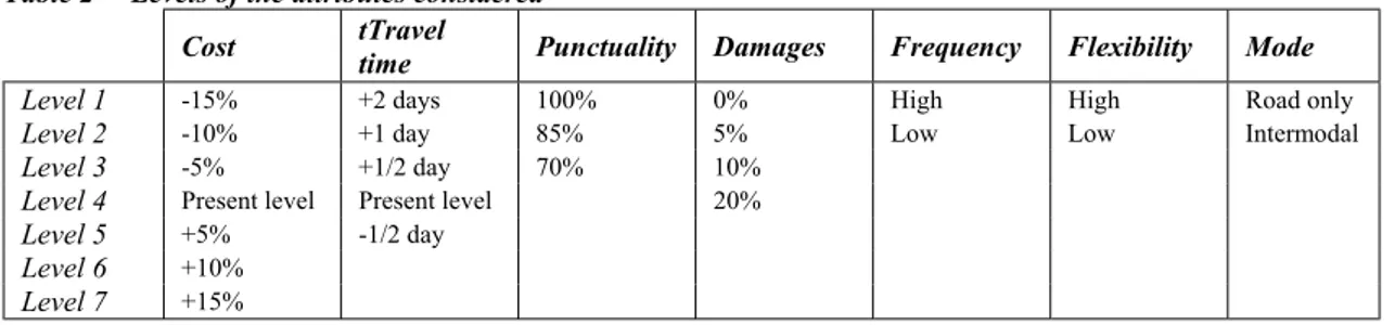
The range of attribute levels employed is reported in Table 2. Table 2 – Levels of the attributes considered
Cost tTravel time Punctuality Damages Frequency Flexibility Mode
Level 1 -15% +2 days 100% 0% High High Road only
Level 2 -10% +1 day 85% 5% Low Low Intermodal
Level 3 -5% +1/2 day 70% 10%
Level 4 Present level Present level 20%
Level 5 +5% -1/2 day
Level 6 +10%
Level 7 +15%
4. Interviews, database and results
The sample was drawn from the list of companies provided by ISTAT and updated in occasion of the 2001 census. The focus was on companies with forty or more employees based on the hypothesis that for these companies it was more likely to clearly locate a person in charge for logistics to be interviewed. The number of employees being a proxy of the companies’ dimension and relevance, the choice made also allowed to restrict the study to those companies with a larger number of shipments and arrivals Restricting the reference population also allows for a higher fraction of it to be sampled. Table 3 reports the total number of companies in the two productive sectors investigated for each province of the Marche region.
Table 3 - Provincial distribution of companies in the DN and DJ sectors
Province DJ DJ % DN DN % AN 154 36,7% 69 19,9% PU 115 27,4% 196 56,6% MC 80 19,0% 65 18,8% AP 71 16,9% 16 4,6% Total 420 100% 346 100%
Table 4 reports the number of companies to be included in the sample for each sector and each Province.
Table 4 - Provincial distribution of companies in the DN and DJ sectors in the sample design
Province DJ DJ % DN DN % AN 19 40,4% 19 24,4% PU 14 29,8% 48 61,5% MC 4 8,5% 7 9,0% AP 10 21,3% 4 5,1% Total 47 100% 78 100%
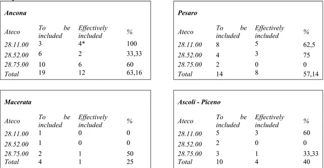
The ratio of companies effectively interviewed for sector DJ is reported, with a province detail, in Table 5.
Table 5 - Provincial comparison between companies to be included and companies effectively included in the sample for the DJ sector
Ancona Pesaro
Ateco To be included Effectively included % Ateco To be included Effectively included %
28.11.00 3 4* 100 28.11.00 8 5 62,5
28.52.00 6 2 33,33 28.52.00 4 3 75
28.75.00 10 6 60 28.75.00 2 0 0
Total 19 12 63,16 Total 14 8 57,14
Macerata Ascoli - Piceno
Ateco To be included Effectively included % Ateco To be included Effectively included %
28.11.00 1 0 0 28.11.00 5 3 60
28.52.00 1 0 0 28.52.00 2 0 0
28.75.00 2 1 50 28.75.00 3 1 33,33
Total 4 1 25 Total 10 4 40
Note: in the case signalled by the symbol * there was an excess of companies interviewed since not all those that were first contacted promptly responded and, while waiting for a reply, they were cautiously not included in the sample and new companies were, in the meanwhile, contacted that were willing to participate to the experiment. Subsequently part of the companies that had not replied decided to participate thus creating the excess.
The ratio of companies effectively interviewed for sector DN is reported, with a province detail, in Table 6.
Table 6 - Provincial comparison between companies to be included and companies effectively included in the sample for the DN sector
Ancona Pesaro
Ateco To be included Effectively included % Ateco To be included Effectively included %
36.11.00 2 2 100 36.11.00 3 2 66,67
36.12.00 6 3 50 36.12.00 10 4 40
36.13.00 5 1 20 36.13.00 7 3 42,86
36.14.00 6 3 50 36.14.00 28 9 32,14
Total 19 9 47,37 Total 48 18 37,50
Macerata Ascoli - Piceno
Ateco To be included Effectively included % Ateco To be included Effectively included %
36.11.00 1 0 0 36.11.00 1 0 0
36.12.00 1 0 0 36.12.00 0 0 0
36.13.00 2 1 50 36.13.00 0 0 0
36.14.00 3 1 33,33 36.14.00 3 1 33,33
A database of 2295 observations was collected by administering 15 choice exercises to each of the 51 companies interviewed.
The choice experiments may or may not include levels of the attributes violating the cutoffs. Table 7 reports the total number of violation for each attribute in the interviews administered.
Table 7 – Cutoffs presence in the choice profiles
Cost Duration Punctuality Damages
Absolute
frequency 390 559 618 1027
Percentage 16,99% 24,36% 26,93% 44,75%
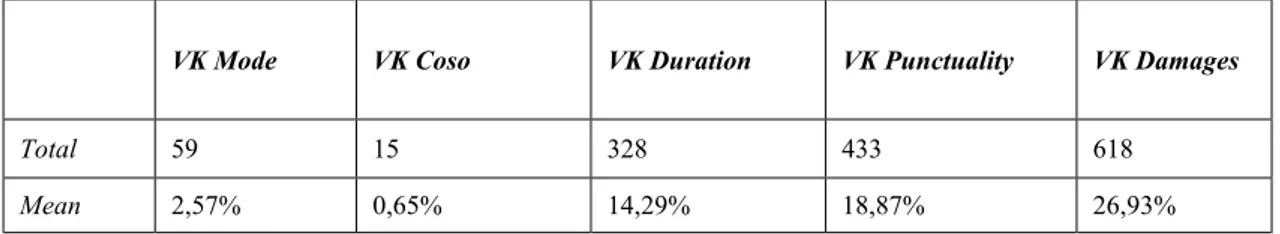
Table 8 illustrates how often an alternative characterised by some cutoff violations has been nevertheless chosen.
Table 8- Number of alternatives chosen characterized by cutoff violations
VK Mode VK Coso VK Duration VK Punctuality VK Damages
Total 59 15 328 433 618
Mean 2,57% 0,65% 14,29% 18,87% 26,93%
Table 9 gives account of the model employed for the estimation of the preferences of the two sectors jointly. The model used is a simple multinomial logit model and was estimated using NLOGIT 3.0 that is part of LIMDEP 8.0 (www.limdep.com). The first model estimated includes, as explicative variables, all the attributes considered. Two dummy variables (assuming the value 1 when the alternative chosen is, respectively, the first or the second one and 0 otherwise) were also included in order to verify the existence of any distortion due to answer position within the choice profile.
Table 9 - LM – All attributes plus dummy one
Variable Coefficient Standard error b/St.Er. p-value
MODE 0,7206 0,2041 3,530 0,0004 CPER -9,7986 0,9022 -10,860 0,0000 DVA -0,2721 0,0934 -2,914 0,0036 PUCH 2,0960 0,5586 3,754 0,0002 DANNI -14,0920 1,3782 -10,224 0,0000 FREQ -0,2024 0,2148 -0,942 0,3460 FLESS -0,3103 0,2152 -1,442 0,1493 A_A -0,8495 0,1698 -5,002 0,0000 A_B -0,8863 0,1753 -5,054 0,0000
Log likelihood function -495,2737
R2 Adg no coefficients 0,4072
R2 Adg constant only 0,2460
Note: MODE = transport mode; CPER = transport cost percentage variation; DVA = transport duration absolute values; PUCH = delivery punctuality; DANNI = damages; FREQ = service frequency; FLESS = service flexibility; A_A e A_B = dummies.
The coefficients are all significant, with the only exceptions of frequency and flexibility, and the relevant explanatory role of cost and damages should be noticed. Concerning the position of the alternatives in the choice profile, it can be seen that the coefficients A_A and A_B are both significantly different from zero but not statistically different from each other. This means that, after accounting for all the other factors, companies tend to choose the third alternative more often than the other two, while alternatives one and two are chosen equally often and no position distortion can be observed for them. The third alternative is, instead, the only “labeled” one, corresponding to the profile with levels of attributes equal to those of the transportation mode currently used. After accounting for all the other factors, companies seem to choose more often the alternative that they actually use. Therefore an alternative specific constant, corresponding to the status quo alternative, was included in the model. Results are reported in Table 10. The estimates of the coefficients clearly resemble those of the previous model.
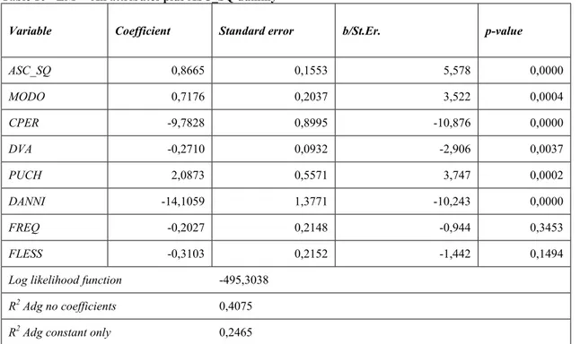
Table 10 - LM – All attributes plus ASC_SQ dummy
Variable Coefficient Standard error b/St.Er. p-value
ASC_SQ 0,8665 0,1553 5,578 0,0000 MODO 0,7176 0,2037 3,522 0,0004 CPER -9,7828 0,8995 -10,876 0,0000 DVA -0,2710 0,0932 -2,906 0,0037 PUCH 2,0873 0,5571 3,747 0,0002 DANNI -14,1059 1,3771 -10,243 0,0000 FREQ -0,2027 0,2148 -0,944 0,3453 FLESS -0,3103 0,2152 -1,442 0,1494
Log likelihood function -495,3038
R2 Adg no coefficients 0,4075
R2 Adg constant only 0,2465
Note: MODE = transport mode; CPER = transport cost percentage variation; DVA = transport duration absolute values; PUCH = delivery punctuality; DANNI = damages; FREQ = service frequency; FLESS = service flexibility; ASC_SQ = actual transport mode dummy .
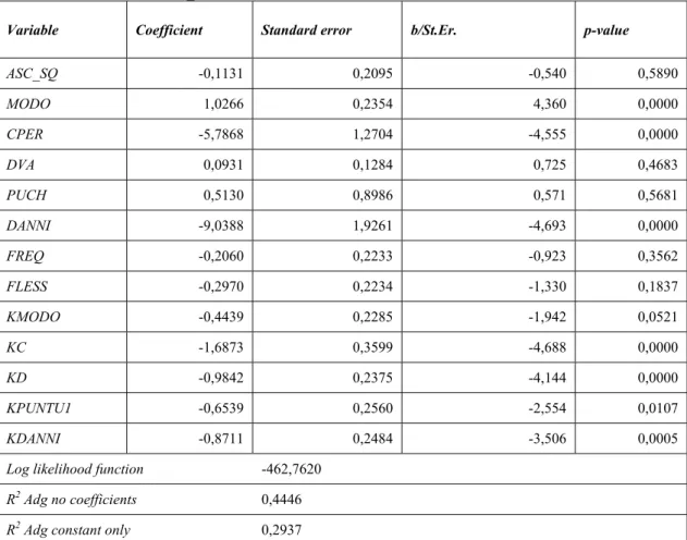
Table 11 – All attributes, ASC_SQ and cutoffs dummies
Variable Coefficient Standard error b/St.Er. p-value
ASC_SQ -0,1131 0,2095 -0,540 0,5890 MODO 1,0266 0,2354 4,360 0,0000 CPER -5,7868 1,2704 -4,555 0,0000 DVA 0,0931 0,1284 0,725 0,4683 PUCH 0,5130 0,8986 0,571 0,5681 DANNI -9,0388 1,9261 -4,693 0,0000 FREQ -0,2060 0,2233 -0,923 0,3562 FLESS -0,2970 0,2234 -1,330 0,1837 KMODO -0,4439 0,2285 -1,942 0,0521 KC -1,6873 0,3599 -4,688 0,0000 KD -0,9842 0,2375 -4,144 0,0000 KPUNTU1 -0,6539 0,2560 -2,554 0,0107 KDANNI -0,8711 0,2484 -3,506 0,0005
Log likelihood function -462,7620
R2 Adg no coefficients 0,4446
R2 Adg constant only 0,2937
Note: MODE = transport mode; CPER = transport cost percentage variation; DVA = transport duration absolute values; PUCH = delivery punctuality; DANNI = damages; FREQ = service frequency; FLESS = service flexibility; ASC_SQ = actual transport mode dummy; KMODO = mode cutoff dummy; KC = cost cutoff dummy; KD = duration cutoff dummy; KPUNTU1 = punctuality cutoff dummy; KDANNI = damages cutoff dummy.
Table 11 clearly shows the strong and significant effect of cutoffs presence. In fact all the cutoffs coefficients are significant and with a negative sign as expected. Their effect on attribute’s coefficients is evident. The coefficients for transport duration and punctuality are no longer significantly different from zero, meaning that, provided the cutoffs on the duration and puntuality are not violated, these two attributes do not have a relevant role in the mode choice. The coefficient of the mode variable increases demonstrating a greater propensity for intermodality, provided the company does not a
priori refuse it. At the same time cost and damages coefficients decrease substantially
given that a relevant part of their effect is now explained through the cutoffs. It is also worthwhile noticing that the coefficient of the status quo variable is no longer significantly different from zero. This means that companies seemed to choose the third alternative more often than the other two only because, obviously, this alternative never includes inacceptable levels of the attributes. Once cutoffs are accounted for, the preference for the status quo alternative disappears.
Log-likelihood substantially increases going from -495,30 to –462,76. The log-likelihood ratio statistic is equal to 65,08, with 5 degrees of freedom and amply confirms that the cutoff coefficients are significantly different from zero and, thus, the last model has better explicative capabilities than the previous one.
Hereafter, the analysis will be carried out allowing for companies in different sectors to have different coefficients for the various attributes. The coefficients for the metallurgic and the furniture sector were estimated on the basis of, respectively, 23 and 28 companies in the sample. The model has been first estimated without taking into account the presence of cutoffs in the alternatives. The results are then compared with those obtained introducing the cutoffs.
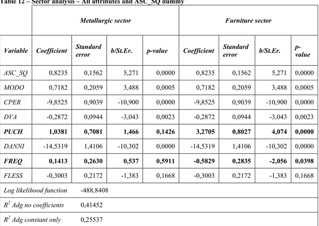
Table 12 shows the sector analysis without cutoffs. As a starting point all the coefficients were allowed to be different in the two sectors. The dimension of the model was then reduced using a stepwise procedure: at each step, all possible reduced models (obtained by constraining, in turn, each coefficient to be the same in the two sectors) are estimated and the one with the highest likelihood is compared to the current model through the likelihood ratio test. If the test turns out to be significant, the current model is considered to be the one which best explains the structure of preferences and the procedure is stopped. Otherwise, if the test turns out to be non significant, the reduced model becomes the new current model and another step is performed. The final model obtained in this way is shown in table 12.
Table 12 – Sector analysis – All attributes and ASC_SQ dummy
Metallurgic sector Furniture sector
Variable Coefficient Standard error b/St.Er. p-value Coefficient Standard error b/St.Er. p-value
ASC_SQ 0,8235 0,1562 5,271 0,0000 0,8235 0,1562 5,271 0,0000 MODO 0,7182 0,2059 3,488 0,0005 0,7182 0,2059 3,488 0,0005 CPER -9,8525 0,9039 -10,900 0,0000 -9,8525 0,9039 -10,900 0,0000 DVA -0,2872 0,0944 -3,043 0,0023 -0,2872 0,0944 -3,043 0,0023 PUCH 1,0381 0,7081 1,466 0,1426 3,2705 0,8027 4,074 0,0000 DANNI -14,5319 1,4106 -10,302 0,0000 -14,5319 1,4106 -10,302 0,0000 FREQ 0,1413 0,2630 0,537 0,5911 -0,5829 0,2835 -2,056 0,0398 FLESS -0,3003 0,2172 -1,383 0,1668 -0,3003 0,2172 -1,383 0,1668 Log likelihood function -488,8408
R2 Adg no coefficients 0,41452 R2 Adg constant only 0,25537
Note: MODE = transport mode; CPER = transport cost percentage variation; DVA = transport duration absolute values; PUCH = delivery punctuality; DANNI = damages; FREQ = service frequency; FLESS = service flexibility; ASC_SQ = actual transport mode dummy . Coefficients which are different for the two sectors are in bold.
The analysis of table 12 seems to show that the furniture sector is sensitive to delivery punctuality and service frequency, while the metallurgic sector is not. None of the sector is sensitive to service flexibility.
Table 13 – Sector analysis – All attributes and ASC_SQ and cutoff dummies
Metallurgic sector Furniture sector
Variable Coefficient Standard error b/St.Er. p-value Coefficient Standard error b/St.Er. p-value
ASC_SQ -0,0297 0,2143 -0,139 0,8898 -0,0297 0,2143 -0,139 0,8898 MODO 0,9983 0,2409 4,144 0,0000 0,9983 0,2409 4,144 0,0000 CPER -4,1001 1,5987 -2,565 0,0103 -8,7051 1,8152 -4,796 0,0000 DVA 0,0809 0,1318 0,614 0,5394 0,0809 0,1318 0,614 0,5394 PUCH -0,0490 1,0298 -0,048 0,9620 2,2223 1,1870 1,872 0,0612 DANNI -5,1732 2,9616 -1,747 0,0807 -13,5652 2,8206 -4,809 0,0000 FREQ 0,2065 0,3013 0,685 0,4932 -0,6812 0,3106 -2,193 0,0283 FLESS -0,3034 0,2297 -1,321 0,1864 -0,3034 0,2297 -1,321 0,1864 KMODO 0,0559 0,3093 0,181 0,8566 -0,9815 0,3292 -2,981 0,0029 KC -2,8979 0,6649 -4,358 0,0000 -0,7971 0,4338 -1,837 0,0662 KD -1,0304 0,2452 -4,203 0,0000 -1,0304 0,2452 -4,203 0,0000 KPUNTU1 -0,5100 0,2699 -1,890 0,0588 -0,5100 0,2699 -1,890 0,0588 KDANNI -1,5964 0,3929 -4,063 0,0001 -0,2412 0,3353 -0,719 0,4719
Log likelihood function -445,7619 R2 Adg no coefficients 0,46258 R2 Adg constant only 0,31649
Note: MODE = transport mode; CPER = transport cost percentage variation; DVA = transport duration absolute values; PUCH = delivery punctuality; DANNI = damages; FREQ = service frequency; FLESS = service flexibility; ASC_SQ = actual transport mode dummy; KMODO = mode cutoff dummy; KC = cost cutoff dummy; KD = duration cutoff dummy; KPUNTU1 = punctuality cutoff dummy; KDANNI = damages cutoff dummy. Coefficients which are different for the two sectors are in bold.
Including the cutoffs in the model makes again a substantial difference. In Table 13 some features, which were completely hidden in the previous model, can now be noticed. First of all, the fact that the two sectors show a quite different sensitivity to costs and damages, with the furniture sector being much more sensitive to these two attributes. This is the main difference between the two sectors and it is completely missed by the model in Table 12, where only the fact that the furniture sector is more sensitive to delivery punctuality and service frequency than the metallurgic one is captured. Notice that the importance of these attributes in differencing the sectors is much reduced in Table 13.
Looking at the cutoffs coefficients it can also be seen that the metallurgic sector has a softer cutoff on the mode of travel compared to the furniture sector. On the other hand, the furniture sector has less rigid cutoffs on costs and damages. In spite of the relevance of these two attributes in the decisional process of the furniture sector, it seems that the
cutoffs of the companies on costs and damages can be compensated for through adequate levels of the other attributes. Finally, both of the sectors show a demand with low compensability for the attributes duration and punctuality. This lack of substitutability implies that a modal alternative must satisfy the companies’ cutoffs on duration and punctuality to have better chances to be taken into consideration.
Finally, notice that the likelihood ratio statistic between model in Table 12 and model in Table 13 is equal to 86,158, with 8 degrees of freedom, leading to the rejection of the null hypothesis that the cutoff coefficients are all zero and, thus, confirming the better fit to the data of the last model.
To conclude this section, with regard to the model presented in Table 13, we calculate some substitution indexes which can help in interpreting the estimates obtained. The substitution index for a generic “non-monetary” attribute X is calculated as
UC UX SIXC ∆ ∆ − =
where is the variation in the utility determined by a unitary variation of the attribute and ∆ is the variation in the utility determined by a unitary variation of the transport cost. Thus, the substitution index indicates how many times a unitary reduction in the cost of transport should be applied to compensate for a unitary variation (perceived as negative) in the attribute . Notice that if the utility function is linear, is simply calculated as minus the ratio between the estimated coefficient of the attribute and the estimated coefficient of the transport cost.
UX ∆ X X UC X XC SI
The following substitution indexes have been calculated:
- which indicates how many times a unitary transport cost discount should be applied in order to compensate a unitary increase in travel time;
TC
SI
- which indicates how many times a unitary transport cost discount should be applied in order to compensate a unitary increase in the risk of late arrivals;
PC
SI
- which indicates how many times a unitary transport cost discount should be applied in order to compensate a unitary increase in damage and loss risk.
DC
SI
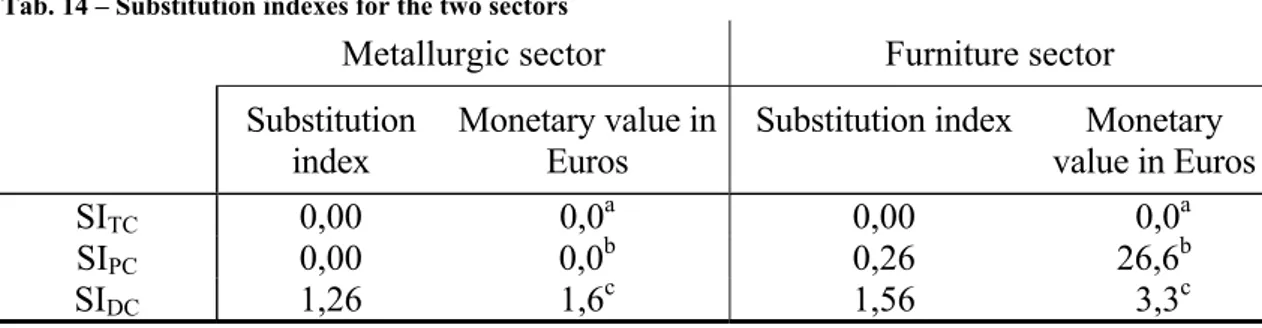
Results are given in Table 14. Notice that the substitution indexes are equal to zero for those attributes with non significant coefficients. The values of travel time and risk of late arrival in euros per hour have been obtained by multiplying the respective substitution indexes for the average cost of transport separately estimated for the two sectors, and then dividing by 12 (considering a travel day made of 12 hours). The value of a 5% risk of damage and loss in euros per thousand euros of transported goods has been instead calculated by multiplying the respective substitution index for the average cost of transport separately estimated for the two sectors, dividing for the average value of transport separately estimated for the two sectors, and then multiplying by thousand and by 5%. Since transports in the two sectors are not homogeneous with regard to travel costs and value of the transported goods, the monetary values reflect, beside other factors, those heterogeneities too.
Tab. 14 – Substitution indexes for the two sectors
Metallurgic sector Furniture sector Substitution
index Monetary value in Euros Substitution index value in Euros Monetary
SITC 0,00 0,0a 0,00 0,0a
SIPC 0,00 0,0b 0,26 26,6b
SIDC 1,26 1,6c 1,56 3,3c
a = value of travel time in Euros per hour b = value of risk of late arrival in Euros per hour
c = value of a 5% risk of damage and loss in Euros per thousand Euros of transported goods
5. Concluding remarks
In this paper compensatory and non compensatory mode choice models with attribute cutoffs analysis have been studied and applied to the case of freight transport in the Marche region with specific reference to furniture and metallurgic productive sectors. Preference elicitation was done using choice based conjoint analysis. The presence and effect of cutoffs violations have been expressly considered and modelled. The overall strong significance of cutoffs parameters demonstrates that not including them in model estimation potentially provokes substantial mistakes.
With specific reference to the sector analysis proposed it is important to underline that there is a substantial difference between the furniture and metallurgic sector consisting of a lower attention, paid by the metallurgic sector compared to the furniture one, to the attributes composing service quality. A further characteristic differentiating these two sectors has to do with the different attitude towards cutoff compensability. Whereas in the furniture sector freight transport demand is more flexible and compensation is sometimes possible even in the presence of ex ante cutoffs (soft ones) the same is not true for the metallurgic sector.
The conclusions drawn from this study suggest that a rethinking of the actual Italian freight transport policy, substantially based on train, ship and intermodality subsidisation, is in order.
Bibliographical references
Borruso, G. e Polidori, G. (a cura di) (2003) Trasporto merci, logistica e scelta modale, Franco Angeli, Milano.
Danielis, R. (a cura di) (2002) Domanda di trasporto merci e preferenze dichiarate -
Freight Transport Demand and Stated Preference Experiments (bilingual), F. Angeli,
Milan.
Danielis, R. and Rotaris, L. (1999) “Analysing freight transport demand using stated preference data: a survey” Trasporti Europei, Anno V, 13, 30-38.
Green, P., Krieger, A., Bansal, P. (1988) “Completely unacceptable levels in conjoint analysis: a cautionary note” Journal of Marketing Research, 25, 293-300.
Louviere, J.J., Hensher, D.A., Swait J.D. (2000) Stated choice methods : analysis and
applications Cambridge University Press.
Maier, G., Bergman, E.M., Lehner, P. (2002) “Modelling preferences and stability among transport alternatives”, Transportation Research Part E 38, 319-334.
Mansky, C. (1977), “The structure of random utility models”, Theory and Decision, 8: 229-254.
Matear, S. and Gray, R. (1993), “Factors influencing freight service choice for shippers and freight suppliers” International Journal of Physical Distribution and Logistics
Management, 23 (2), 25-35.
Ortuzar, J. e Willumsen, L. (1994), Modelling Transport, Wiley, Chichester.
Polidori, G. e Marcucci, E. (2003) “Domanda di trasporto merci e preferenze dichiarate: il caso delle Marche”, in: Trasporto merci, logistica e scelta modale, Borruso, G. e Polidori, G. (a cura di), Ed. Franco Angeli, Milano.
Swait, J.D. (2001) “A Non-compensatory Choice Model Incorporating Attribute Cutoffs” Transportation Research: Part B: 35 (10) 903-28.