Analytical invariants of conformal transformations : a dynamical system approach

cAi

)oK

I

^

UNIVERSITAT DE BARCELONA

ANALYTICAL INVARIANTS OF CONFORMAL TRANSFORMATIONS.

A DYNAMICAL SYSTEM APPROACH

by

V.G. Gelfreich

AMS

_{Subject Classification:}

_{58F23, 58F35}

Mathematics _Preprint

_{Series No.}

₂₂₉

Analytical Invariants of Conformal

Transformations.

A

_dynamical

_system

_approach.

V. G. Gelfreich

February

4,

1997

Abstract

The _{paper is devoted to the problem of analytical classiñcation of} conformal _{maps of the form /:zt-)-z+z2+...inaneighborhood ofthe} degenerate fixed point z = 0. It is shown that the analytical invariants,

constructed in the works of Voronin and Ectille, may be considered as a

measureof the_{splitting for stable and unstable (semi-)invariantfoliations} associated with thefixed_{point. Thissplitting appearstobe exponentially} small with respect to the distancetothe fixed point.

The _{problem of local classiñcation of analytic morphisms} on the complex

plañe (C,0) seems to be solved completely at the present time. The classical

result is that a _{morphism / : z *-4 Az + ... with A ^ 0 and |A| ^ 1 can be}

conjugated with its linearpart z Az. ThecaseofaresonantA (thereisn £ N,

such that A” = 1) _was solved independently by J.Ecalle [1] and S.Voronin [2]. In this case there is a countable number of _{independent quantities which are} invariantwith _{respect to analytical changes of coordinates.}

In the _{present paper we concéntrate our attentionon the case A}= 1 and re-peat the results of[2], usingadynamicalsystemapproach tothe problem. This givesus ageometricinterpretationofthe obstacles for the analytic conjugation,

which are _quite similar _to the phenomenon of the splitting of separatrices in 2D Hamiltonian _{Systems. In the latter class ofsystems the splitting leads to} a

chaotic behavior of trajectories. In the case of analytic maps on the complex

plañe it provides obstacles for analyticity only.

In the present paper we give a new method for construction of the basic Solutions for the Abel _{equation (see Section 2). This method is based on the}

theory offinite-difference equations proposed in [3, 4], In Section 3 the

rela-tion between _{analytic invariant and dynamics is discussed. And in Section 4}

a numerical method for computing the analytic invariant for _a given _map is

provided.

1

_{Analytical classification by Voronin}

Firstwerecall some results from the _{paper [2]. Let/ denote afunction analytic}

at zero,

f : z z+

z2

+az3+

0(z4).

(1)

The problem is when for two given functions of this form, / and /, there is a

diffeomorphism h, such that f =hofoh~x ina neighborhood ofz = 0.

Any map / with /'(O) = 1 and /"(O) ^ 0 can be transformed to the form

(1) by a linear h. The coefficient a is invariant with respect to any h, which

can be represented as a (formal) power series in z, h(z) = z+ .... There is not

any other formal invariant since an application of the form (1) can be formally

conjugated to the polynomial

m 2+z2+

az3,

₍₂₎

but,ofcourse, the corresponding series diverges in general.

In _{[2] acomplete set of analytic invariantswas constructed with the help of}

twobasic Solutions Ai and A2 of the Abel equation

A(f(z)) = A(z) + 1. (3)

The functions Ai andA2 are analytic respectively in the domains

Si = { |argz| _{< 7r}-

¿}

nDr, S2 = { | arg(-z)| < n-S }nDr,

where Dr = {|z| _< r}. It is assumed that r is sufficiently small. Moreover,

Ak{z)=-l/z +o{l/z) (4)

on their domains. In particular, A* transform asectorial neighborhood of the

origin into asectorial neighborhood of theinfinity. Consider the function4>(í) = A2o

_Aíl(t).

_Dueto

(4)

and

(3)

it is well defined for sufficiently large

|Im<|

and

$(* + !)= $(<)+ !. (5)

Thus, it may be continued into two half-planes II± = {( S C : ±ImC > R}

provided the constant Rissufficiently large. Let

= A2_oAj

1

n± (6)

The functions Ai and A2 are defined by (3) and (4) uniquely up to additive

constants. _{Consequently, the functions <£±} are defined up to a substitution

$±(C) = $±(C + ai) + a2, where ai

and

a2 are

arbitrary complex

numbers.

This relation provides an equivalence inthe set of pairs of analytical functions.

The _{equivalence class of (<J>+,<Í>_) is said to be an analytical invariant of the} function /.

Indeed, let h be an _{analytical function at theorigin, h'(0) = 1, and consider}

the function _{/ = hofoh~l. The Solutions of the Abel equation, which}

corre-spond to/, aregiven by A/, —A* oh. The analytical invariant of the function

/, given by

4>= A2 _°

Aj"1

_{= (A2 oh) o}(Ai _o

h)~1

_{= A2o}

Af1

_=<J>,

coincides with the _{analytical invariant of the function /.}

Theorem 1 _{[2]. Twofunctions of the form (1) are analytically conjugated in} a neighborhood _{ofzero if}and only if their analytical _{invariants coincide.}

The_{equations (5) and (4) imply that the functions $-¡- may be represented} in the form

OO

*±(*) = *+

&£

+

£ ó±e±2l>fct,

₍₇₎

k=1

where theFourier series_{convergeandgotozero as|Imf | —¥ 00in the half-planes}

n±, respectively. In [2] it was shown, that for any pair of analytical functions of the form _{(7) it is possibleto construct afunction (1), such that the pair is a}

representative of its analytical invariant.

Example. An important example is the function

fo(z) = = z-T

z2

+

z3

+• • • • (8)

Inthis case the Abel _{equation has an obvious globally defined solution}

A(z) =

-I.

We _{maychoose A+(z) = A-(z) = A(z). Consequently, $(<) = t. That is the}

analytic invariant of this function is trivial, in the sense that = 0 for all

k> 1.

In the coordínate t = —I¡z the _map /o is _a translation _{í H ¡ +} 1. The

trajectories belongtostraight linesIm(<) =const. Corning back tothe variable

z we see that these lines are transformed into circles, _{which pass through the}

origin,with horizontaltangent onit. These circles areinvariant with respect to

the _map

/o-An _arbitrary mapofthe form (1) has asimilar (local topological) structure

of_{trajectories since it may be topologicallyconjugated with /o [5].}

2

Construction

of

inverse Abel functions

Instead of the Abel _equation we will study the equation

z(t+ l) = f(z(t)) (9)

Figure 1: Domains ofdefinition for the inverse Abel functions, Í2_ and fi+.

Lemma 2 The _{equatíon (9) has a uniqueformal solution of the form}

i

₊

íL^sí+feS^fl.

_k—3

„o)

where_{pk stands for a polynomial of degree less than k. In the case ofa = 1 all}

Pk are ofdegree zero, i.e., they are constant.

The _{proof ofLemma 2 isstraightforward (see e.g. [1]).}

Lemma 3 For_{anyJo > 0 there is} apositivenumber R, such that the equatíon

(9) has two Solutions, z~(t) and

z+(¿),

analytic in thesectors ÍI_ = { | arg(z+

R)| > Jo} andÍI+ = { | arg(z—ií) —n\ > Jo}, respectively, and which have the

asymptotic expansions (10).

The rest of the section contains the _{proof of Lemma 3. First,} we need

someelementary facts on thetheory of finite-difference equations, which afford

us to rewrite the finite-difference equatíon (9) as an “integral” one and use a

contraction map principie in properly chosen functionalspace.

2.1 Linear finite-difference

_equations

In the _present section we study the problem of inverting the linear

finite-difference _operator

2

L(w)(t) = w(t -I-1)— w(t)—

jw(t).

This operator plays the role of an approximation for the variational equatíon

associated with _{(9). First,} we need a solution of the homogeneous equation

L(wq) = 0. Obviously,

We look for a solution of this _{equation in the form wo(t) =}

eu°^\

_The substi-tution into the _{equation gives}

«0(t + 1) - Uo(0 = log ■

The function _uo(t) = log((í+ 1)t) satisfies the last equation, and we

immedi-ately get the desired solution for the homogeneous equation:

w0(t) =t(t + 1). (11)

Now we can solve the _{nonhomogeneous equation}

Lw= /,

where _{/ is a known function, which decreases fast enough at infinity. We use} the method of variation of_{parameterslooking for the solution in the form}

w(t) = C{t)w0{t).

Substitution into the _{equation gives}

(C(t+ 1) — C(t))wo{t + 1) = /(<)•

This_{equationhas twoSolutions}

“

f(t ~*)

“»o(< +

!-*)’

c-(o =

E

c+(t) - _y'

+

t'ow^t+i+ky

Taking into account (11) we get the final expression for the Solutions of the

nonhomogeneousequation w _(t)

w+(t)

tu+

dY

*?

_í(í +1)

y

t*)

(< + 1+k)(t+2+ k) fe=o (12) (13)

The series converge provided / =

0(td)

with d < —2 for |í| —¥ oo and then w=

0(td~l).

Let

T^íl*)

denote the Banach_space

of

analytic

functions in

Q*,

which are continuousin the closure, with the norm

ll/IU =

sup|íd/(OI-n±

It is easy to see that the equations (12) and (13) define two bounded linear operators L¿¿ ->

which solve

the equation Lw

=

f in

the

2.2 Proof of Lemma 3

Welook for the solution of the _{equation (9) in the form}

,±

-o

W--J

₊

(1- q) logt

í2 +w(t).

The first two termsin the_{right-hand side of the last equation satisfythe equation}

(9) with an error

0(t~4).

Thus, substituting into the equation (9) we get

w(t+ 1) =

^1

+

w(t)

+

g(t)

+

t),

(14)

where

g(t) =

0(t-4),

/(O, t) = 0,

|^(0,0

=

0(r2logí).

Inverting the linear operator we obtain from (14)

MO =

(Ld,±a)

(<)

₊

')

(*)•

Choosing d = 3 — S, S € (0,1), it is not difficult to prove the existence and

uniqueness ofasolution for the last equation by the contraction mapprincipie. An _{analogous estímate maybe found in [3, 4],}

3

Invariant

foliations

Considering the images of the lines Imí = const with respect to

z±,

weobtain

(semi) invariant foliations. Wesaythat z~ defines theunstable foliation, and

z+

defines the stableone. _{Originally, the unstable solution oftheequation (9), z~,} is defined on the domain Q_ only. But if the function / is entire, the function

z~ maybe analytically continued on the whole complex plañe by iterating the equation (9). The restriction of the mapz~ on Í2_ isone-to-one ontoits image, but, in general, that is not true for the analytical continuation. Thecase ofz+

is_{different, since}onehastocontinué thefunction z+ tothe left from itsoriginal

domain of_{definition,Í1+ (see Fig. 1). To do thatone needs aninverse function}

f~1. The map / is invertible in a neighborhood ofz = 0, but it may have no

global inverse.

For _{/(z) = /o(z) = z/(l — z) we have}

_z+(t)

_{= z~(t) — —l/t, and the} invariantfoliations consist of circles and cover the whole _{complex plañe C.} Of

course, the stable and unstable foliations coincide in thiscase.

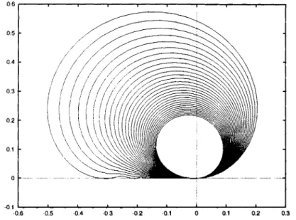
In _{general, the stable and unstable foliations do not coincide (Fig. 2): the}

lines, leaving a neighborhood of the origin in a regular way, donot come back

in the same _{way. The difference consists of the phase shift, described by the}

Figure 2: Unstable foliation for the quadraticmap z>-> z+

z2,lmt

goes through

the interval

_[0.05,3)

_{with the step 0.1.}

oscillations are _{exponentially small with respect to the imaginarypart of the}

parameter í. The later is approximately the inverse of the diameter of the corresponding invariant quasi-circle in the plañe of z-variable.

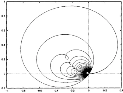
In_{Figure 3wepresent theunstable foliation forthecubicmap 2}

_z+z2+z3.

It isseenthat forsmall valúes of Imí the_{corresponding lines of unstable foliation} have self intersections duetothe_{passage nearthecritical pointz =}

_{(—1+\/2)/3.}

The_{Une, which} passes through the critical point has cusps.

The _{lines, which} start in with small valué of|Imí|, may have a

compli-catedcontinuation _{as, forexample, in Figure 4.}

Now we _{study the splitting of the stable and unstable foliations, i.e., we}

comparethe lines, which coincide formally. Consider z+(t) and z~(t) for Imí = tr, o- 1. We assume that the branches oflog are chosen in such a way, that

the _{asymptotic expression (10) gives the samevalúes for}

_z+(í)

_and

_z~(t)

_{in the}

upper half-plane. The last hypothesis makes no restriction, since the change

of the branch is_{equivalent to a substitution í *->■< + (1 — a)2ink, k £ Z. The} diñerence _{z+(t) — z"(í) decreases faster than any powerof}

_í-1

_{as Imí —► +oo.}

In _{particular, that implies that the correspondingrepresentative ofthe analytic}

invariant has noconstant term:

<Mí) = í+

£6+e2-fct.

₍₁₅₎

k=1

correspon--0.5 -0.4 -0.3 -0.2 0.1 0 0.1 0.2 0.3

Figure 3: Unstable foliation for the cubicmap z z+

z2

+

z3:

Imt £ (1.8,4.8).

Figure 4: Continuation of the line of the unstable foliation for the cubic map

dence between the linesofthe stable and unstable foliations.

Proposition 4 Let the mapf have the following coefficients in the expansión

(15)

6+ = 6+ = ... =

6+_1

= 0,

6+^0,

for some positive mteger n, then for all sufficiently large cr > 0 the lines z+(t)

and_{z~(t), Imí = a, intersect along 2n trajectories of the map f, andfor any}

ofthese trajectories the intersectionangle is given by

a =

27m\b+\e-2nna

₊

0(e-2^n+1)a).

Ifb+ = 0 for alln, then the stable and unstable foliations coincide forlmt > 0.

Note, that the angle has thesame valuéat all points ofahomoclinic trajectory,

because _{the map / is conformal. The iterates ofahomoclinic point accumulate}

to the _{origin, consequently, if6+ ^ 0 forsome n, then the line z~(t) (as well as}

z+(í)),

Imí = cr 1, is aclosed real-analytic line (asymptoticallyacircle), but

it is not differentiable at the _origin.

It is _{remarkable, that forany map / ofthe form / : z t-+ z +}

_z2

_{+ ... there}

are _{only two possibilities:}

1. the _{angle is exponentially small with respect to a = Imí and behaves}

asymptotically like

27m|6+|e-2,rr*<T,

2. it is _identicallyzero andthe stable and unstable foliations coincide.

The _{splitting of the stable and unstable foliations produces no chaotic} be-haviorof_{trajectories: the map / is topologically conjugated to z►-* z/(1 — z).} An _{analogous study} maybe done in the Iower half-plane Imí < 0. Thetype

of the _{splitting in the Iower half-plane is independent of the behavior in the}

upper half-plane, and any combinationmayappears.

Proof ofProposition 4■ Wefix S > 0 and consider the sector S < arg z < n— ó. We take í = _{Ai =}

(z+)-1

_{as a coordínate in this sector. Then the stable}

foliation is _{given by Imí = <r and the unstable foliation can be represented in} the _{parametric formí = $+(¿<r+r), r 6 R. The line of the unstable foliation} intersects Imí= a _provided

Im _{($+(¿cr-(- r)) = cr.}

Taking into account (15) we get

Im

OO

e—2nkcr+2iirkT

.k=n

where we used that

£>^

_{= ... =}

6+_j

_{= 0. Since 6+ ^ 0 weget}

r arg

6*

2mi +

¿+0(e-2-).

¿n (16)

Since in the coordínate t the _{map / acts as t >-»• t + 1, we have 2n distinct} homoclinic _{trajectories.}

Since the line of the stable foliation is horizontal the intersection _{angle at a} homoclinic _{point isgiven by}

Im_{<&+(i<T+ r)}

tana = :

Re$+(í<7+ r)

where r is_{given by (16) and the point denotes the derivative withrespect to t,}

Using again (15) we get

OO Im

_{^2b+2inke-2*k‘’+2i*kT}

tana =

^

=

±2nn\b¿;\e-2*n°

+

0(e~2^n+1^).

1 + Re

_{b^2ÍTrke~2nk,7+2inkT}

k=n

Since the _{map z+ is conformal itpreserves angles, and the angle of intersection} of the lines of the stable and unstable foliations is described _{by the}sameformula in both z- and í- variables.

4

_{Computation of analytical invariants}

We _{investígate numerically the analytical invariants forsome maps.} The _{analytic invariant (6) is given bythe function}

$(<) = A2oz~(t).

The functions A2 may be fixed by the following asymptoticcondition

A2 =-- 4-(1 - a)logz+ a„zn, z ->■0, zeS2- (17)

2

n>i

The coefficients an are defined uniquely from the Abel equation (3). If f(z) is

realfor real z then these coefficients are real numbers. Comparingthis asymp¬

totic with ₍₁₀₎ weobtain that = ±(1 —a)n.

The other coefficients

_bf

_{can not be obtained from these asymptotic}

ex-pansions only because the Fourier series in (7) decrease exponentially fast with

We note that

(18)

$(<) = A2 o

f2n

02 (í— n) — n

for all n € N. Here _f2n denotes the compositionof 2n functions /.

Thesequence f2noz~(t—n) — fnoz~(t) goes to zero in the sector S2 as n goes to infinity provided |Im<| is not toosmall. Consequently, we can evalúate

the function _{$(í) in the followingway: choose n sufficiently large and calcúlate}

z~_{(t — n) using a finite part of the sum (10); apply 2n times the map / tothe}

obtained _point; use a finite part of the asymptotic expansión (17) to get the approximatevalué of<í>(¿).

Fouriercoefficients in ₍₇₎canbe evaluated using the usual formula forFourier

coefficients

¿>± = exp(27T<rfc)

í

($± (±i<x₊ r) _{— (±i)<7}

— r)exp(q=27rikr)dr (19)

Jo

where a > 0 is afixed number.

In the _computations we used the asymptotic formula (17) with the error

term _being

_0(z4)-

_{The integral in (19) was computed by rectangular formula}

with 16_{equidistant nodes. This method provides sufficiently high accuracy and}

is stable with _{respect to} a and n.

The results of the_{computation of the first Fourier coefficient for the} polyno-mialmap z >->■ z+z2 usingdifferent valúes ofaand n aregiven in the following

table.

tT n _{IC1 1}U+l

_argcf

3.5 100 22350579.12 2.9733955458 4.5 100 22350589.2 2.9733953515 6.0 100 22350580.22 2.9733953361 3.5 500 22350579.22 2.9733955202

Moreover, we find out numerically that

_|6^|

of the polynomial (2) depends

on a _{asymptoticallyasconst •}

exp(—27r2a)

_{fora —► —00.}

5

_{Acknowledgments}

The author thanks V. F. Lazutkin for _{attracting the author attention to the}

problem. The author also thanks Caries Simó for many important remarks

and the _{department ofApplied Mathematics and Analysis of the University of} Barcelonafor the _hospitality.

References

[1] J. Ecalle, Les fonctions resurgentes, vol. 2, Publ. Math. d’Orsay, (1981) [2] S. M. Voronin, Analytical classifications of conformal maps (C,0) —> (C,0)

with identical linear parts, Fuñe. Anal. Appl. (1981), vol. 15, no. 1, 1-17 (Russian)

[3] Lazutkin V.F., Exponential splitting of separatrices and an analytical in¬

tegral for the semistandard map, (1991), preprint of Université París VII,

53 _p.

[4] Gelfreich V., Conjugation to ashift and splitting of invariant manifolds, to

appear in Applicaciones Matematicae (Warsaw).

[5] M. Yu. Lyubich, Dynamics of rational transformation: topological picture,

Relació

deis últims

_Preprints

_publicáis:

210 On the relationship between a-connections and the asymptotic properties of predictive

dis-tributions. J.M. Corcuera and F. Giummolé. AMS 1980 Subjects Classifications: 62F10, 62B10, 62A99, July 1996.

211 Global efficiency. J.M. Corcuera and J.M. Oller. AMS 1980 Subjects Classifications: 62F10, 62B10, 62A99. July 1996.

212 Intrinsic _{analysis of the statistical estimation. J.M. Oller and J.M. Corcuera. AMS 1980}

Subjects Classifications: 62F10, 62B10, 62A99. July 1996.

213 A characterization _{ofmonotone and regular divergences. J.M. Corcuera and F. Giummolé.} AMS 1980 _{SubjectsClassifications: 62F10, 62B10, 62A99. July 1996.}

214 On the_{depth of the}fibercone offütrations. Teresa Cortadellas and SantiagoZarzuela. AMS Subject Classification: Primary: 13A30. Secondary: 13C14, 13C15. September 1996.

215 Anextensión _{of Itó’sformula foranticipating}processes. Elisa AlósandDavid Nualart. AMS

Subject Classification: 60H05, 60H07. September 1996.

216 On the contributions of Helena Rasiowa to Mathematical Logic. Josep María Font. AMS

1991 _{Subject Classification: 03-03,01A60, 03G. October 1996.}

217 A maaimal_{inequality for the} Skorohod integral. Elisa Alós and David Nualart. AMS Subject

Classification: _{60H05, 60H07. October 1996.}

218 A _{strongcompletenesstheorem for the Gentzensystemsassodated with finite algebras.}

_Ángel

_J.

Gil, Jordi Rebagliato andVentura Verdú. Mathematics SubjectClassification: 03B50, 03F03,

03B22. November 1996.

219 Fundamentos dedemostración automática de teoremas. Juan CarlosMartínez. Mathematics

Subject Classification: 03B05, 03B10, 68T15, 68N17. November 1996.

220 _{Higher Bott Chem forms and Beilinson’s regulator. José Ignacio Burgos and Steve Wang.} AMS _{Subject Classification: Primary: 19E20. Secondary: 14G40. November 1996.}

221 On the _{Cohén-Macaulayness of diagonal subalgebras of the Rees algebra. Olga Lavila. AMS}

Subject Classification: 13A30, 13A02, 13D45, 13C14. November 1996.

222 Estimation _{ofdensities and applications. María Emilia Caballero, Begoña Fernández and} David Nualart. AMS _{Subject Classification: 60H07, 60H15. December 1996.}

223 _{Convergence within nonisotropic regions of harmonio functions in Bn. Carme Cascante and}

Joaquín Ortega. AMS Subject Classification: 32A40, 42B20. December 1996.

224 Stochastic evolution _{equations with random generators. Jorge A. León and David Nualart.} AMS _{Subject Classification: 60H15, 60H07. December 1996.}

225 Hilbert _{polynomials over Artinian local rings. Cristina Blancafort and Scott Nollet. 1991} Mathematics _{Subject Classification: 13D40, 14C05. December 1996.}

226 Stochastic Volterra equations in the plañe: smoothness of the laui. C. Rovira and M.

Sanz-Solé. AMS _{Subject Classification: 60H07, 60H10, 60H20. January 1997.}

227 On the Cohén-Macaulayproperty of the fiber cone of ideáis with reduction number at most

one. Teresa Cortadellas and_{SantiagoZarzuela. AMSSubject Classification: Primary: 13A30}

Secondary: 13C14, 13C15. January 1997.

228 Construction _{of 2mSn-fields containing aC-i*-field. Teresa Crespo. AMS SubjectClassific¬}