POLITECNICO DI MILANO
SCHOOL OF INDUSTRIAL AND INFORMATION ENGINEERING
MASTER OF SCIENCE IN MANAGEMENT ENGINEERING
Buckingham Theorem Application to Machine Learning Algorithms:
Methodology and Practical Examples
Relator: Prof. Giovanni Miragliotta
Academic year: 2018/19
Master Thesis of:
Federico Frisone – 899389
2
Ringraziamenti
Prima di procedere con la trattazione, vorremmo dedicare qualche riga a tutti coloro che ci sono stati vicini in questo percorso di crescita personale e professionale.
Un sentito grazie al nostro relatore prof. Giovanni Miragliotta per la sua disponibilità e tempestività ad ogni nostra richiesta.
Senza il supporto morale dei nostri genitori e familiari, non saremmo mai potuti arrivare fin qui. Grazie per esserci sempre stati soprattutto nei momenti di sconforto.
Ringraziamo i nostri colleghi e amici per esserci stati accanto in questo periodo intenso e per gioire, insieme a noi, dei traguardi raggiunti.
3
Table of Contents
Sommario ... 9 Abstract ... 10 Extended Abstract ... 11 Introduction ... 11Objectives of the thesis project ... 12
Theoretical background ... 13
Buckingham Theorem ... 13
Machine Learning... 15
Literature review main findings ... 15
Methodology proposal for the application of BT to ML ... 17
Practical cases ... 20
Artificial Neural Network ... 20
Clustering ... 24
Conclusions ... 27
Introduction ... 28
1.1 Machine Learning... 28
1.1.1 Machine Learning: overview ... 29
1.1.2 Challenges of high-dimensional data ... 30
1.1.3 Feature Selection and Feature Extraction ... 31
1.1.4 Principal Component Analysis ... 33
1.2 Buckingham Theorem ... 34
1.2.1 History of the theorem ... 34
1.2.2 Phi-Theorem: Key Concepts ... 35
1.2.3 Buckingham Theorem benefits ... 39
1.2.4 An illustrative example... 40
1.2.5 Dimensional Analysis and Features Extraction ... 42
1.3 Thesis project description ... 43
2 Literature Review ... 45
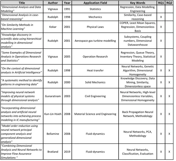
2.1 Method of Analysis ... 45
2.2 Papers ... 47
4
2.3.1 Considerations on potential BT application to ML ... 74
2.3.2 Benefits ... 75
3 Methodology for Buckingham Theorem in Machine Learning ... 77
3.1 Conditions of applicability (Step 1) ... 79
3.2 Computation of dimensionless variables (Step 2) ... 80
3.2.1 Knowledge-based Approach ... 80
3.2.2 Explorative Approach ... 81
3.2.3 Iterative Approach ... 81
3.3 Further processing of dimensionless variables (Step3) ... 83
3.3.1 Domain Independent techniques ... 83
3.3.2 Domain Dependent techniques: creation of dimensionless hypervariables ... 84
3.4 Feeding the algorithm and evaluating performances (Step 4) ... 85
4 Practical Cases ... 86
4.1 Artificial Neural Networks ... 86
4.2 Dimensional Analysis application to a regression model ... 88
4.2.1 Dataset Description ... 89
4.2.2 Knowledge-based Approach (ANN) ... 90
4.2.3 Explorative Approach (ANN) ... 91
4.2.4 Conclusions (ANN) ... 95
4.3 Clustering ... 95
4.3.1 Introduction to clustering ... 97
4.3.2 Methodological considerations on Clustering application ... 100
4.3.3 Dataset description ... 102
4.3.4 No Da Application ... 105
4.3.5 DA Application: Explorative approach ... 108
4.3.6 Conclusions (Clustering) ... 111
5 Conclusions ... 114
6 References ... 117
5
Table of Figures
Figure 1 - Methodology of BT to ML……….…18
Figure 2 – Dimensionality influence on Classifier performances ... 30
Figure 3 – Data Density with Feature increase ... 31
Figure 4 – Matrices for dimensionless numbers computation ... 37
Figure 5 – Shock Absorber System ... 41
Figure 6 – Variables in the Shock Absorber System ... 41
Figure 7 – Schematic description of hierarchical modeling ... 50
Figure 8 – Approximation function schematic representation ... 52
Figure 9 – Schematic representation π-transform ... 52
Figure 10 – Bar of length l under load q ... 53
Figure 11 – Homogeneous ANN ... 54
Figure 12 – Case Based Reasoning process ... 57
Figure 13 – Shock Absorber System ... 58
Figure 14 – Data mining for patterns discovery phases ... 60
Figure 15 – DA in data mining for patterns discovery ... 60
Figure 16 – Schematic approach for DA in ANN ... 62
Figure 17 – PCA in ANN layers ... 68
Figure 18 – NPCA in autoassociative neural network ... 69
Figure 19 – Pressure calculated by Flowline Pro and OLGA ... 72
Figure 20 – Temperature calculated by Flowline Pro and OLGA ... 72
Figure 21 – Methodology for DA application in ML ... 78
Figure 22 – Main dimensionless numbers in fluid dynamics ... 80
Figure 23 – Artificial Neural Network ... 87
Figure 24 – Hierarchical clustering ... 98
Figure 25 – Elbow indicator ... 99
Figure 26 – Iris scatterplot ... 103
Figure 27 – Cases analyzed in clustering ... 104
Figure 28 – Elbow indicator in No DA Application ... 105
Figure 29 – Silhouette diagram in No DA Application ... 105
Figure 30 – Scatterplot No DA Application ... 106
Figure 31 – Silhouette diagram in No DA Application with Further processing ... 107
Figure 32 – Scatterplot in No DA Application with Further processing ... 107
6 Figure 34 – Scatterplot Explorative Approach ... 109 Figure 35 – Silhouette diagram after hypervariables computation ... 110 Figure 36 – Scatterplot after hypervariables computation ... 111
7
Table 1 – Mpg Dataset ... 20
Table 2 - ANN results ... 22
Table 3 - Clustering results ... 25
Table 4 - Clustering results and Benchmark evaluation results ... 26
Table 5 – Matrix for dimensionless number computation in Shock Absorber System ... 42
Table 6 – Research papers classification ... 46
Table 7 – Variables in a Shock Absorber System ... 58
Table 8 – Cases stored in the database ... 59
Table 9 – Value of query data ... 59
Table 10 – Variables in spin coating of thin films in IC industry ... 63
Table 11 – ANN performances in five different representations ... 67
Table 12 – Cases analyzed ... 88
Table 13 – Dimensional matrix in MPG Auto ... 90
Table 14 – ANN results ... 94
Table 15 – Clustering results ... 112
8 Eq. 1 ... 13 Eq. 2 ... 13 Eq. 3 ... 36 Eq. 4 ... 36 Eq. 5 ... 38 Eq. 6 ... 38
Eq.8 Hypervariables computation ... 84
9
Sommario
L'era dell'informazione è caratterizzata da una crescente disponibilità di dati. In questo contesto, il Machine Learning è una tecnologia intersettoriale all'avanguardia che offre la possibilità di ottenere insight, riconoscere e creare modelli predittivi a partire dai dati. Tra le sfide poste da questa impressionante disponibilità di dati, una delle più rilevanti è quella di avere a che fare con insiemi di dati composti da un elevato numero di attributi.
Nell'ingegneria classica, il teorema di Buckingham, basato sull'analisi dimensionale, viene utilizzato per ridurre il numero di variabili che descrivono un problema fisico. Alcuni autori hanno fornito esempi dell'applicazione combinata di algoritmi di Analisi Dimensionale e Machine Learning, evidenziando i principali benefici ottenuti.
Viene presentata una metodologia che fornisce percorsi alternativi per l'implementazione del teorema nel campo del Machine Learning. In primo luogo, vengono descritte le condizioni che un dataset deve soddisfare per essere adeguato all'applicazione del teorema. In secondo luogo, vengono illustrati i possibili approcci e le relative tecniche per il calcolo e l'ulteriore trasformazione di numeri senza adimensionali, che sono l'input per l'algoritmo di Machine Learning. Un ruolo critico per la selezione del percorso è svolto dalla conoscenza del problema affrontato nel dominio dell'analista.
Vengono presentati due esempi pratici dell'implementazione della metodologia per il clustering e per modelli di regressione. I risultati ottenuti sono consistiti in: una riduzione delle variabili necessarie per descrivere i problemi, un aumento dei valori delle metriche di performance e una semplificazione della struttura degli algoritmi.
10
Abstract
The Information Age is characterized by an increasing availability of data. In this context, Machine Learning is a cutting-edge cross-sectoral technology providing the possibility to obtain insights, to recognize patterns and to create predictive models from data. Among the challenges brought by this impressive availability of data, one of the most relevant is dealing with datasets composed of a high number of attributes.
In classical engineering, the Buckingham Theorem, based on Dimensional Analysis, is used to reduce the number of variables describing a physical problem. Some authors provided examples of the combined application of Dimensional Analysis and Machine Learning algorithms, pointing out the main benefits achieved.
A methodology providing alternative paths for the theorem implementation in Machine Learning field is presented. First, the conditions that a dataset must satisfy to be adequate for the theorem application are described. Secondly, the possible approaches and related techniques for the computation and additional transformation of dimensionless numbers, which are the input for the Machine Learning algorithm, are illustrated. A critical role for the path selection is played by the analyst domain knowledge of the addressed problem.
Two practical examples of the methodology implementation for clustering and prediction purposes are presented. The obtained results consisted of: a reduction of the variables needed to describe the problems, an increase in values of performance metrics and simplification of algorithm structure.
11
Extended Abstract
Introduction
Stepping into the information age means an increasing availability of data. This condition is mainly due to decreased storage costs, increased availability of computing power at lower costs and proliferation of new sources of data (e.g. IoT, social media, digitalization of processes in companies and public institutions). Machine Learning (ML) provides the possibility to obtain insights, to recognize patterns and to create predictive models from data. The increased availability of data entails some challenges. Specifically, difficulties in identifying relevant variables and redundant information arise when dealing with high-dimensional datasets (i.e. high number of variables). Another issue related to the high dimensionality of datasets is that as the number of features increases, the amount of data needed to generalize accurately grows exponentially. Moreover, there is an increasing need for optimizing computational processes. In this context, dimensionality reduction techniques are used to overcome the aforementioned problems. Among these techniques, two categories can be identified, namely, Feature Selection and Feature Extraction.
In classical engineering, a consolidated technique for dimensionality reduction is the Buckingham Theorem (BT), based on Dimensional Analysis (DA). BT states that a functional equation involving n physical variables f( x1, x2, ..., xn) = 0 described by k physical dimensions, can be represented by a set of p = n − k dimensionless parameters πi, derived from the original dimensional variables, in the form F( π1, π2, ..., πp ) = 0. The consolidated benefits of the theorem result from the reduction of the number of variables used to analyze the problem and from the insightful description of the phenomenon provided by the physical meaning of the dimensionless variables generated.
12
Objectives of the thesis project
In the context presented in the previous paragraph, the first goal (Research Question 1) of this
thesis project is understanding if Dimensional Analysis can represent a value-added approach when applied to Machine Learning algorithms. To answer this question, DA and
ML have been studied at first separately, to get the required knowledge of both topics. Then, papers discussing DA application combined with ML algorithms, have been researched and analyzed.
Authors that contributed to the topic provided interesting insights and examples of approaches. However, these contributions have never been organized in a structured form. Therefore, the main cues and information concerning the topic dealt with by the thesis are presented in an organized way. In the second part of the work, the goal (Research Question 2) is to extract a
general step by step methodology for Dimensional Analysis application to Machine Learning algorithms, integrating the main contributions of the existing literature.
Once drafted, the methodology has been tested through two practical examples of its implementation. Therefore, the third part of the work (Research Question 3) is composed of
two applications of the methodology combined respectively with Artificial Neural Networks and K-means clustering algorithm.
13
Theoretical background
Buckingham Theorem
The Buckingham Theorem states that any dimensionally homogeneous1 equation can be written as a functional relation among a complete set of dimensionless independent products. In a problem involving one dependent variable and n-1 independent variables, related by a function
f, the following equation can be written:
𝒙𝟏= 𝒇(𝒙𝟐, … . , 𝒙𝒏);
Eq. 1
This means that the BT allows grouping the original variables to generate p = n – k (where k is the number of fundamental quantities through which other variables are described) dimensionless products πi related through the function F.
𝝅𝟏= 𝑭( 𝝅𝟐, … , 𝝅𝒑)
Eq. 2
Quantities of a problem are called fundamental if they can be assigned a unit of measurement independently from the units of measurement used for the other fundamental quantities of the problem. Length, time and mass are examples of such quantities. Otherwise, they are called
derived quantities. This distinction is not necessarily fixed. It is under the responsibility of the
researcher to understand the most suitable set of fundamental quantities depending on the typology of the analyzed phenomenon.
When applying the BT, it is necessary to make sure that only one functional relation f exists among the variables. Moreover, no relevant quantities can be left out of the analysis and/ or extraneous quantities included. Therefore, a complete set of independent dimensional variables must be identified. There are some variables, essential for the problem description, that have a constant value, like the Gravitational Constant g. They must be anyway included in the set of n variables describing the problem. In case the selected variables do not respect the independency and completeness condition, the BT might not provide any substantial benefit. It is easy to
1Dimensional homogeneity is the quality of an equation having quantities of same units on both sides (Cimbala and
14
understand that a good level of domain knowledge is required to effectively apply the theorem.
Dimensionless variables are computed following an algebraic technique (Langhaar, 1951). From an initial set of dimensional variables, it is possible to derive different sets of independent dimensionless products. As a result of the technique proposed by Langhaar, π1 (Eq. 2)must be the only dimensionless group containing the dimensional and dependent target variable x1.
Once the function F has been experimentally or theoretically identified, the dimensional target variable x1 is easily deduced through a simple algebraic computation. Benefits deriving from
BT application are:
- Reduction of the number of variables involved: the immediate result of the DA application is
the reduction of the number of variables describing the problem. This often leads to a simplification of the necessary procedures in the analysis.
- Identification of similarities: another relevant benefit is the construction of models in scale.
Indeed, transforming the dimensional variables into πi terms, it is possible to make analysis and tests on a reduced model. The concept underlying similarity is that two distinct data pointsin the dimensional space (n dimensions) are represented by the same data point in the dimensionless space (n-k dimensions) if they have the same values of dimensionless numbers. This is valid because the dimensionality reduction represents a surjective mapping function.
- Higher domain knowledge: the application of BT is also an opportunity for the researcher to
get insights on the general principles ruling the analyzed phenomenon. Thanks to the interpretation of the physical meaning of πi terms, some relations and dependencies between dimensional variables and target variable can be highlighted.
15
Machine Learning
Machine Learning algorithms are usually applied with the purpose of extracting useful knowledge to support decision-making processes. ML is based on inductive learning methods, whose main goal is to derive general rules starting from a set of available past observations and then generalize these conclusions. ML techniques are applied in several domains, such as recognition of images, texts analysis, medical diagnosis and relational marketing.
Based on the presence of a target attribute, the learning process of ML may be defined as supervised or unsupervised. In the first case, the target attribute expresses for each record either the membership class or a measurable quantity. Classification and regression models belong to this category. In the second case, no target attribute exists and consequently, the purpose of the analysis is to identify regularities, similarities, and differences in the dataset. Association rules and clustering belong to this category.
Typically, when a supervised ML algorithm is applied, the analyzed dataset is split into two subsets. The first one (training set) is made of a sample of records extracted from the original dataset, and it is used to train the algorithm for the learning model definition. Then, the predictive accuracy of each alternative model generated can be assessed using the second subset (test set), in order to identify the best model for future predictions.
Literature review main findings
Among the authors focusing on DA application in ML, the first one is Rudolph (1998; 2000) who provides a description of data mining process phases and of the steps where DA can be implemented. Moreover, the author shows how DA can reduce both the number of features (columns) and samples (rows). In another research, Rudolph analyzes the concept of dimensional homogeneity and its related issues in regression models. The author shows how to overcome these problems through the implementation of the BT embedded in the designing process of an Artificial Neural Network (ANN).
Kokar (2000) proposes an approach valuing the quality of the set of dimensionless numbers feeding a regression model. Specifically, the author emphasizes the importance of selecting the set (π1, π2, ..., πp ) that best describes the phenomenon.
16
dimensionless groups describing the phenomenon (called dimensionless hypervariables). The potential benefits achievable are a further reduction of the dimensionless variables and increased algorithm performances. Moreover, the set of dimensionless hypervariables might have a significant physical meaning for the problem description.
Kun-Lin (2008) lists a series of fundamental steps to incorporate DA and ANN to process modeling in the concrete industry. The author provides numerical evidence of the benefits coming from the BT application.
Bellamine (2008) illustrates how to combine Principal Component Analysis and DA within the design of an ANN.
Ove Bratland (2019) provides an example of a combination of DA, mechanistic model and ANN to improve the development of mathematical models for two- and three-phase flow in long pipelines.
After having described the authors’ contributions, it is valuable proceeding analyzing the possible benefits and advantages brought by Dimensional Analysis to Machine Learning, extracted by the literature review. The BT guarantees a reduction of the dataset equal to the number of dimensions characterizing the problem. The higher the number of dimensions involved in the problem, the higher the impact of the reduction of dimensionality resulting from the BT application. The term ‘reduction’ must not be confused with ‘elimination’ since the features of the dataset are recombined generating a new dataset keeping the same information content. The reduction in the number of attributes leads to additional advantages. Since the model has fewer degrees of freedom, the likelihood of overfitting is lower. Therefore, the model will generalize more easily. It also helps remove redundant features, if any, and takes care of multicollinearity, improving the model performances. Moreover, dimensionality reduction helps in data compression, since the algorithm training is characterized by lower computational time and space. Finally, if the dataset is sufficiently reduced, it is possible to implement Machine Learning algorithms (e.g. K-means) that typically unfit for large datasets.
Referring to the papers which worked on DA and applied it to ANN, it is evident that the BT leads to a simplification of the ANN topology since the dimensionless groups embed part of the phenomenon non-linearity. Moreover, the reduction of the number of variables leads to a lower number of nodes in the first layer.
17
Concluding, the analyzed papers make the Dimensional Analysis an interesting and valuable tool when dealing with dimensional datasets. However, the literature did not show a unique approach for Dimensional Analysis application in the Machine Learning field.
Considering the listed and described benefits, a clear answer to the first research question (RQ1) emerges. The evidence of the benefits brought by Dimensional Analysis, when combined with Machine Learning algorithms, justify a further research effort to integrate and organize the already existing scientific contributions.
Methodology proposal for the application of BT to ML
The outcome of the integration of the literature contributions is a methodology tree describing the possible options that can be followed when applying DA to ML algorithms. The method can be considered as part of the preprocessing phase. In addition, assumptions and considerations of the first step of the methodology are only related to characteristics the dataset must satisfy to be considered adequate for BT application. Therefore, the designed method is valid disregarding the class and typology of the algorithm used. In Fig. 1, each step is illustrated within the boxes and the alternative options are named together with the authors that most provided a contribution in terms of approach and/or technique.
18
Figure 1 -Methodology of BT to ML
In Step 1, the conditions of applicability of the theorem, that the dataset variables must satisfy, are evaluated. If the conditions are verified, the dataset can be considered appropriate for the application of DA.
19
Step 2 consists in the dimensionless number computation. This is a task that can be carried out through three alternative approaches. The first approach is the Knowledge-based Approach. In this case, the analysis of similar problems already solved and previous experiences are the main sources to get insights about the problem and then identify a possible set of πi dimensionless variables. The second approach is the Explorative Approach whose objective is to get the best performing set of dimensionless variables, searching in the space of all the possible sets obtainable, applying the matrix technique. The third and less common approach is the
Iterative Approach, presented by Rudolph (1998) for ANNs. It carried out through a genetic
algorithm that generates individuals differing only for the parameters characterizing the network topology. Finally, only the ANNs that satisfy the BT and a predetermined performance value summarized by a fitness function, survive. Given the homogeneity issue and computational effort required, this approach has not been included in the practical application. Moreover, the genetic algorithm does not allow the researcher to be involved in the dimensionless number computation and selection since they are automatically calculated by the genetic algorithm. This is clearly the opposite of what discussed by authors as Taylor who values the role of the researcher in the BT implementation.
In Step 3, further transformations of the πi terms are proposed to obtain additional benefits in
terms of number of variables and algorithm complexity. Among the possible transformations, two macro-categories can be identified: Domain Independent techniques and Domain
Dependent techniques. As for the first category, when applying these techniques, it is possible
to combine input variables using different methods to generate a new reduced set that often has not a dimensional meaning, and that leads to potential loss of information and homogeneity issues. The most widely used technique among the Domain Independent ones is Principal Component Analysis (PCA). As an alternative to Domain Independent techniques, it is possible to further process the dimensionless terms generating dimensionless hypervariables.
Hypervariables are formed as a product of πi terms (except for the dimensionless target variable) raised to different exponents (−1, 0, 1), analyzed in pairs, as shown below:
{𝜋
𝑖; 𝜋
𝑖𝜋
𝑗(𝑗 > 𝑖);
𝜋
𝑖20
This enlarged representation space is then pruned using sensitivity information to select the best performing set of hypervariables. The pruning process is constrained by specific criteria identified by Gunaratnam (2002) that must be satisfied. Generally, the creation of
hypervariables is driven by the need for furtherly reducing the dimensionality of the πi set, and by the possibility to obtain a deeper knowledge of the problem and to improve the algorithm performances. Therefore, this approach can be considered valuable when dealing with a high number of πi.
No specific clue on the algorithms’ structure and performance evaluation (Step 4) is discussed since it is not part of the work objectives.
Practical cases
Artificial Neural Network
The problem analyzed consists of the prediction of the miles travelled by a car with a gallon of fuel, based on the vehicle's technical features. The problem is tackled following the steps of the methodology proposed in the preceding paragraph. The dataset used for the practical application is MPG Auto, from the UCI repository. Following the physical description of a very similar problem provided by Vignaux (2001), but not tackled using ML algorithms, a complete set of dimensional variables and parameters adequate satisfying the applicability conditions of BT (Step 1) is identified in Table 1.
Table 1 – Mpg Dataset
The approaches for the computation of the dimensionless numbers presented in the methodology are explored (with the exception of the genetic algorithm) and compared to the case in which DA is not implemented. In each case, Domain Independent (represented by PCA) and Domain
Dependent (represented by hypervariables computation) techniques are alternatively applied to
achieve an improvement of the algorithm performances. ANNs have been exploited to generate the regression model because ANN is the algorithm used in most of the works presented in the literature review.
21
For the computation of the dimensionless variables (Step 2), the Knowledge-based Approach and the Explorative Approach are applied and the further processing techniques (Step 3) are implemented for each approach.
Knowledge-based Approach
A complete description of the problem is provided by Vignaux (2001). He denotes a set of significant dimensionless numbers. π1=
𝑚𝑝𝑔 𝑤 𝑔 𝑒 π2= ℎ 𝑤√𝑙𝑔3 π3 = 𝑇√ 𝑔 𝑙
Feeding the ANN with π1, π2, π3, categorical (origin) and additional numerical variables (cylinders and model year), the combination [Knowledge-based Approach; No Further
processing] of Table 2 is analyzed. The first approach proposed to further process the
dimensionless variables is the Domain Independent (PCA technique). Feeding the ANN with principal components obtained after PCA application, categorical the combination
[Knowledge-based Approach; Domain Independent] of Table 2, at the end of the paragraph, is
analyzed. The second approach proposed to further process the dimensionless variables is the
Domain Dependent one. π2 and π3 are combined and the resulting set of hypervariables is then pruned through a sensitivity analysis. The most performing combination of dimensionless
hypervariables is represented by the pair (π2; π5= π2/ π3). Feeding the ANN with π1, π2, π5, categorical and additional numerical variables, the combination [Knowledge-based Approach;
Domain Dependent] of Table 2 is analyzed. Explorative Approach
As an alternative to the Knowledge-based Approach, the Explorative Approach (Step 2) is presented in methodology. Applying the algebraic technique, 15 possible sets of dimensionless variables are generated. Each set has been used as input to feed the ANN, whose performances have been evaluated. At the end of the abovementioned process, the best set is selected. It corresponds to the columns order (mpg,g,l,h,w,e,a) and is composed of:
πa= 𝑚𝑝𝑔 𝑒 √ ℎ𝑤 𝑡 πb= 𝑔 √ 𝑤𝑡 ℎ πc= 𝑙𝑤 ℎ√𝑡3 .
Among them, πa is the most significant one. It embeds all the technical features of the vehicle providing a compact insight on vehicle efficiency. The higher the value of πa, the higher the
22
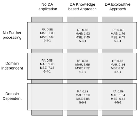
efficiency. Feeding the ANN with πa, πb, πc, categorical and additional numerical variables the combination [Explorative Approach; No Further processing] of Table 2 is analyzed. Feeding the ANN with the principal components, obtained after PCA application, and the categorical variable, the combination [Explorative Approach; Domain Independent] of Table 2 is analyzed. Applying the Domain Dependent Approach, the following set of hypervariables is generated {πb; πc; πd = πb πc; πe = πb/πc}. Any pair of hypervariables πi have not improved the performances of the algorithm compared to the values obtained with πb, πc. Among the other combinations, the best performances were achieved by πe alone, reducing in this way the number of input variables. Feeding the ANN with πa, πe, categorical and additional numerical variables, the combination [Knowledge-based Approach; Domain Dependent] of Table 2 is analyzed. For each analyzed case, values of R2, Mean Squared Error (MSE) and Mean Absolute Error (MAE) together with the best ANN topology are displayed.
Table 2 - ANN results
As the reader can verify, the Explorative Approach with No Further processing has provided the best value for all three metrics.
The application of the DA (Explorative Approach and Knowledge-based Approach) led to an improvement of the performances compared to the No DA application case and to a reduction of the number of input variables. It also increased the knowledge of the phenomenon, because
23
the physical meaning of πa provided a comprehensive and compact description of the problem. These outcomes are consistent with the expectations. In fact, a reduction of the number of variables involved is guaranteed by the BT. Moreover, embedding the non-linearity of the problem in dimensionless terms, the algorithm performances are improved. It is reasonable to achieve better results in the Explorative Approach because the best performing set was selected as a result of the exhaustive research of the dimensionless sets space.
The application of Domain Independent techniques in the combination [No DA Application,
Domain Independent] improved the ANN performances, reducing the input features. In the
combination [Knowledge-based Approach, Domain Independent], PCA resulted in slightly worse performances in terms of MAE, but furtherly reducing the variables of the problem. Finally, when applied to the Explorative Approach, PCA produced a significant topology simplification but with a relevant drop in the performances. The reduction of performances resulting from PCA application to dimensionless variables can be traced back to the relevance of each πi for the problem description. This means that eliminating part of the knowledge embedded in an already reduced set of variables through Principal Components Analysis, the capability of predicting the target variable decreases. On the contrary, when PCA is applied to a non-reduced set of dimensional variables, it increases the overall performances.
The generation of hypervariables (Domain Dependent) led to better performances both in the
Knowledge-based Approach and Explorative Approach. In the former case, the Domain Dependent technique improved the performances, while in the latter it brought to a further
reduction of the input variables with a small drop of model accuracy. It is possible to state that also in this case a further reduction of the best set of πi (Explorative Approach) did not lead to better accuracy. This is due to the fact that, as already said for the Domain Independent
Approach, the optimal set of dimensionless variables can hardly be additionally improved.
However, given the negligible drop in accuracy, the advantage of furtherly reducing the number of variables makes the creation of hypervariables a successful technique.
24
Clustering
The main drivers suggesting that DA might provide benefits when combined with clustering algorithms are the opportunity to exploit the similarity concept in the BT and the possibility of reducing the dimensionality of input datasets. Moreover, DA allows lowering the number of variables without losing the possibility to interpret the set of dimensionless variables describing the space where clusters are identified and qualified. It is important to underline by shifting to clustering problems, the dataset completeness condition (Step 1) can be relaxed since expanding or reducing the number of features of the dataset, it is possible to identify different meaningful solutions depending on the input data. As a consequence, the domain knowledge of the researcher plays an even more important role. In fact, the absence of a method to identify a complete set of variables makes the domain knowledge a crucial resource to find the most relevant attributes for the clustering analysis.
In order to verify the potential benefits of DA in clustering problems, the proposed methodology has been applied to Iris dataset. The choice of the dataset was driven mainly by its wide usage in the academic fields and for its simple structure. It consists of measurements of 150 Iris flowers divided into three different species: Iris Setosa, Iris Versicolor and Iris Virginica. Four features were measured from each sample: the length and the width of the sepals and petals. The features of the dataset are characterized by one fundamental quantity, the length [L].
The clustering algorithm has been evaluated according to two different approaches. The first one takes into account the metrics commonly used to evaluate clusters. The second one considers also the label (species) as a good benchmark solution to evaluate the clusters identified. It is important to underline that also in the second approach (benchmarking with belonging species) the learning process is completely unsupervised because labels are only used in a final evaluation step to understand if the resulting clusters are well defined or not, without adjusting the obtained clusters according to the corresponding label.
As it emerges from the scatterplot of the labeled observations, there are clearly two distinct and concentrated groups of data points. One composed of Setosa class elements, and the other one where the observations of Versicolor and Virginica class are partially overlapped. Among the possible algorithms, the K-means has been chosen because consistent with the dataset
25
characteristics. The methodology has been implemented in the clustering problem, except the
Knowledge-based Approach. In fact, given the limited number of variables of the dataset, the Explorative approach has been preferred to the Knowledge-based Approach, because a
negligible computational effort was required to explore the research space of all the possible dimensionless set. The overall amount of cases analyzed is five (Table 3).
Explorative Approach
Using the Langhaar technique, 4 dimensionless variables sets have been generated and used to feed the K-means algorithm. The best one has been selected to analyze the case [Explorative
Approach, No Further processing].
During the case [Explorative Approach, Domain Dependent technique], the hypervariables have been generated using the dimensionless set of the preceding case and analyzed through sensitivity analysis. The set of dimensionless hypervariables identifying clusters characterized by high values of SC and DBI was: {π2 =
𝑝𝑒𝑡𝑎𝑙 𝑙𝑒𝑛𝑔𝑡ℎ sepal length , π3 =
𝑝𝑒𝑡𝑎𝑙 𝑤𝑖𝑑𝑡ℎ sepal length}.
From an inspection of the scatterplot and the silhouette diagram, it emerged that one cluster is clearly separated from the others, while the remaining two are partially overlapped. However, the DA transformation allowed a better distribution of the data points laying in the mixed (dimensionless) space, compared to the previous cases.
26
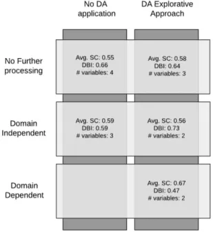
Table 3 summarizes the overall metrics values for each case analyzed implementing the methodology. Considering the values of Silhouette Coefficient (SC), Davies Bouldin Index (DBI) and number of features, the most adequate solution for the clustering analysis is the one obtained in the Explorative Approach enhanced by the generation of hypervariables (Domain
Dependent technique). DA enhanced by Domain Dependent technique led to a significant
improvement of the principal metrics and a reduction of the number of variables. Moreover, it is possible to state that a simple DA application brought to better results if compared to a traditional K-means application without data processing. In contrast, DA without further processing led to worse results if compared to a Feature Selection technique on the dimensional dataset. Table 4 summarizes the results benchmarked to species labels. It is evident from a quick evaluation of the results, that the best performances are again obtained in the cases [Explorative
Approach, No Further Processing] and [Explorative Approach, Domain Dependent techniques]. The results are a practical evidence that DA might provide the possibility to better
identify homogeneous groups of observations in the dimensionless space rather than in the dimensional one. In fact, the transformation of the space performed by the DA allows to better distinguish the clusters associated with the label ‘VERSICOLOR’ and ‘VIRGINICA’ that appear mixed and more hardly distinguishable in the dimensional space.
Table 4 - Clustering results and Benchmark evaluation results
cluster 1 cluster 2 custer 3
SETOSA 50 0 0
VERSICOLOR 0 50 0
VIRGINICA 0 0 50
cluster 1 cluster 2 custer 3 cluster 1 cluster 2 custer 3
SETOSA 50 0 0 50 0 0
VERSICOLOR 0 48 2 0 45 5
VIRGINICA 0 14 36 0 2 48
cluster 1 cluster 2 custer 3 cluster 1 cluster 2 custer 3 cluster 1 cluster 2 custer 3
SETOSA 50 0 0 50 0 0 50 0 0
VERSICOLOR 0 46 4 0 46 4 0 46 4
VIRGINICA 0 0 50 0 0 50 0 8 42
Benchark solution
No DA Application Filtering Method
27
Conclusions
Evidence of the potential benefits provided by DA, when applied in ML field, have been presented and discussed in the literature review. A methodology resulting from the integration of the main contributions of analyzed papers has been drafted. On one hand, the methodology is a tool to guide the ones that have no knowledge of the BT application to ML algorithms. On the other hand, it provides an ordered approach for those that already use the BT in their data analysis processes.
To support the methodology, two practical cases have been shown respectively referring to ANN and K-means algorithm. The former one allowed to explore, step by step, the alternative paths presented in the methodology. The latter one represents the starting point for new possible applications of the DA in ML. In both cases, numerical evidence of the benefits of BT have been obtained. Specifically, an increase in performance metrics, a reduction of the number of variables and a consequent simplification of the algorithm structure have been achieved. Moreover, in the ANN practical case, the dimensionless variables brought an increased knowledge of the phenomenon, thanks to a compact representation of the problem.
It is important to underline that the domain knowledge is a fundamental prerequisite since the choice of fundamental quantities and dimensional variables is crucial for the effectiveness of the BT implementation.
When no significant computational constraints are in place, a complete exploration of the possible sets of dimensionless numbers is suggested. Otherwise, the support of experts and previous works can be considered a valid and faster way to identify dimensionless numbers characterizing the problem.
Therefore, it is reasonable to state that any time a researcher approaches a problem for which the BT conditions of applicability are satisfied, the use of the presented methodology can lead to relevant benefits.
28
Introduction
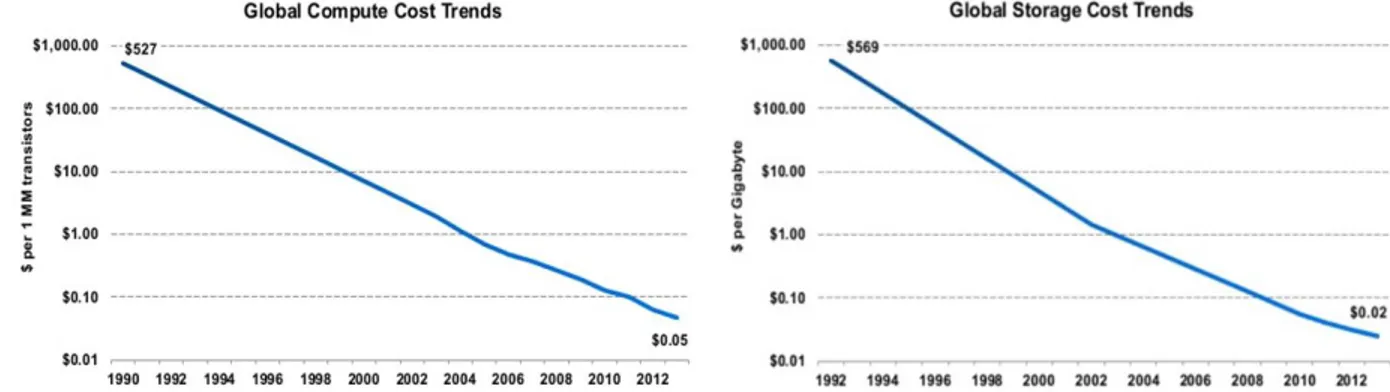
Stepping into the information age means an increasing availability of data. Sensors present in the multitude of objects used every day by ordinary people and in industrial processes, social media constantly updated and monitored, and public institutions that are going through a process of digitization, are generating an ever-increasing amount of data. At the same time, two consolidated trends are driving the explosion of such a phenomenon:
• Decreased storage costs; • Decreasing compute cost.
Figure 2 – Compute and storage costs
1.1 Machine Learning
Machine Learning is a subfield of Artificial Intelligence. The goal of ML is extracting useful knowledge from data supporting in this way the decision-making process. Algorithms used in the ML field build a generalizable model able to make predictions and find patterns in datasets. ML techniques are applied in several domains. Examples of daily applications are traffic predictions, virtual personal assistants, email filtering or product recommendations. Wide usage of ML algorithms is also present in the manufacturing industry for predictive maintenance, quality control, logistics, and stock management.
Learning processes can be classified in supervised or unsupervised according to the presence of a target variable. In the first case, the value of a target variable can express a quantity or a class that must be predicted. Classification and Regression are part of this category. In the second case, the aim of the algorithms used is not related to the prediction of values but to the recognition of patterns, regularities, and similarities. Clustering and Association Rules belong to this category.
29
1.1.1 Machine Learning: overview
In supervised learning processes, the dataset used is typically divided into two subsets. One, called training, is used to identify the best values for parameters of the algorithm. The other, called testing, is used to evaluate performances. A third subset can be used before the testing phase to reduce risks of overfitting, it is called validation dataset.
A brief description of the main classes of learning processes, based on the work of Vercelli (2009) is presented hereafter to provide the reader with an overview of the possible tasks that can be tackled using ML techniques.
Regression: The aim of regression models, also called explanatory models, is to identify a
functional relationship between the target variable and a subset of the remaining attributes composing the dataset. The most used algorithms for regression analysis are linear and multilinear regression, support vector, random forest regressor, and neural networks.
Time-series: The aim of the time series is analyzing dataset composed of data in which the target
variables are time-dependent and are associated with sequences of consecutive periods along time. The value-added of this approach lies in the possibility to predict the values of the future period according to data related to the past period.
Classification: This typology of learning process is based on the labeling present in the dataset
expressed by a categorical variable. Each data point presents a feature describing the belonging class of the element. The goal is to identify the most probable label for each element in the dataset. The most used algorithms for classification analysis are logistic regression, nearest neighbor, support vector machines, decision trees, random forest, and neural networks.
Association rules: The objective of association rules is detecting patterns and recurring
combinations of items. They are for example used to determine suggested products according to the already purchased ones.
Clustering: Clustering algorithms are used to identify groups of homogeneous elements within
a dataset. The clusters obtained can be considered well identified if they have high internal homogeneity and high external heterogeneity.
30
1.1.2 Challenges of high-dimensional data
Big data brought significant benefits in several industries like manufacturing, healthcare, communication, entertainment, banking, insurance, and others. The drawback of dealing with such a huge amount of data, often coming from different sources, is the increased complexity in data management and knowledge extraction. The main resulting issues are:
• Difficulties in identifying relevant variables; • Presence of redundant information;
• Increasing need for optimizing computational processes.
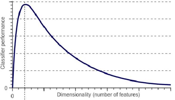
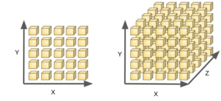
These arising challenges can be even emphasized by a poor knowledge of the domain the data belongs to, and by an unstructured methodology to approach data analysis. The enormous proliferation of data is characterized not only by a high number of samples present in the available datasets, but also by a high number of attributes (i.e. dimensions). In those datasets, the number of attributes (n) is comparable in terms of quantity to the number of elements (m). Often, among the several attributes in high-dimensional datasets only a small number embeds relevant information and it is critically important to correctly identify them. Adding attributes to the dataset can increase the performances of the algorithm because more information can be exploited. However, as shown in Fig.2, over a certain number, adding more variables can be detrimental to the algorithm’s results.
Figure 2 – Dimensionality influence on Classifier performances2
2The Curse Of Dimensionality in Classification Vincent Spruyt -
31
Moreover, as the number of features (dimensions) grows, the amount of data needed to generalize accurately grows exponentially. This happens because more data must be present to get a comparable data density in the space in which the research is carried out (Fig.3).
Figure 3 – Data Density with Feature increase3
1.1.3 Feature Selection and Feature Extraction
In data mining processes and business intelligence, the dimensionality of datasets is generally reduced to mitigate the aforementioned implications. The main benefits of dimensionality reduction are:
• Accuracy improvements;
• Overfitting risk reduction;
• Algorithm training speed-up;
• Data Visualization enhancement;
• Model comprehension increase.
A first distinction within the dimensionality reduction techniques can be made between Feature
Selection and Feature Extraction techniques. The former ones reduce the number of variables
through a selection of the attributes that best describe the problem analyzed, eliminating those attributes that are not considered relevant for the data mining process. The latter ones transform the original attributes generating a reduced set of new variables resulting from the combination of the starting ones. The main drawback related to Feature Selection is the loss of all the information embedded in the removed variables. The principal drawback associated with the
3Escaping the Curse Of Dimensionality Peter Gleeson -
32 Feature Extraction is the loss of interpretability of the handled dataset resulting from the
transformation.
Feature Selection techniques are usually subdivided into three categories:
• Filter methods select the relevant variables before the learning (or training) phase and
are for this reason independent from the algorithm used. Attributes are ranked according to specific metrics and the most significant are selected for the training phase, while the others are discarded. A very common and simple method belonging to this group is the correlation analysis, through which the most correlated variables are selected to train a model. Being the most rapid and less burdensome from a computational standpoint,
Filter Methods are commonly applied to large datasets;
• Wrapper methods use the algorithms applied in the learning phase to find the most
relevant variables. Iteratively, one different subset of variables is used to train the model. Finally, the one that has the best performances is chosen. Usually, this group of methods is applied in regression or classification problems where accuracy is the metric to assess the performances of the subsets of attributes. It is evident that an exhaustive research through the whole space of possible subsets that implies the generation, learning and testing of each attribute set is computationally expensive. Therefore, a wrapper method is suggested anytime the researcher is dealing with a small dataset and low time and cost constraints;
• Embedded methods present the selection of relevant variables inside the algorithm in
order to choose the optimal set of variables directly in the model generation phase. An example is represented by Classification Trees that automatically select the relevant variables for the classification task.
Feature Extraction Techniques, as already pointed out, have the peculiarity of transforming the
starting variables to get a new representation of the data points. These methods are used to reduce the dimensionality of the dataset limiting the amount of lost information.
A not trivial drawback is that the combination of initial variables are usually hard to be interpreted. The most known Feature Extraction techniques are:
33
• Principal Component Analysis (PCA); • Independent Component Analysis (ICA); • Linear Discriminant Analysis (LDA); • Locally Linear Embedding (LLE); • Autoencoders.
For the purpose of the present work, PCA is described to provide the reader with a basic knowledge of its usage, benefits, and limits.
1.1.4 Principal Component Analysis
Principal component analysis (PCA) is the most widely known technique for attribute reduction by means of projection. It is used to reduce the dimensionality (i.e. the number of variables) of a data set consisting of many variables correlated with each other and typically used to lower issues like over-fitting in high dimensional space. The purpose of this method is to obtain a projective transformation that replaces the original numerical attributes with a lower number of new attributes generated as linear combination of the former ones. The analysis starts by standardizing the dataset. It is important to standardize the features since they can be of different scale and can contribute significantly towards variance. Denoting X the standardized dataset, let V be the covariance matrix of the attributes. Principal components are related to the eigenvalues and eigenvectors of the covariance matrix V. The principal components are obtained by means of the eigenvector uj, associated with the maximum eigenvalue λj of V, through the relation pj = Xuj. Each eigenvalue expresses the amount of variance explained by each principal
component.
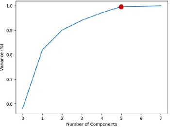
There are as many principal components as variables. The n principal components constitute a new basis in the space Rn, since the vectors are orthogonal to each other. They can be ordered according to a relevance indicator expressed by the corresponding eigenvalue. In particular, the first principal component explains the greatest proportion of variance in the data, the second explains the second greatest proportion of variance, and so on. However, often only the first q principal components are used. The value q can be deduced using a number of heuristics, but most often a scree plot of the eigenvalues is obtained, and the location of the ‘elbow’ is considered to be the optimal q (Fig. 4). Principal components are better suited than the original attributes to explain fluctuations in the data, since a subset consisting of q principal components,
34
with q < n, has an information content that is almost equivalent to that of the original dataset, without the issues arising from a large number of variables. As a consequence, the original data are projected into a lower-dimensional space of dimension q having the same explanatory capability.
Figure 4 – Principal components explained variance
1.2 Buckingham Theorem
The aim of the present paragraph is to give a high-level overview of the Buckingham Theorem (BT), also known as Phi-Theorem, in order to provide the reader with a basic knowledge to understand the concepts covered in this thesis project.
The theorem states that a functional equation involving a certain number of n physical variables
f (x1, x2, ..., xn) = 0 described by k physical dimensions, can be represented by a set of p = n - k
dimensionless parameters derived from the original dimensional variables, in the form F (π1, π2,
..., πp ) = 0. The BT leverages the Dimensional Analysis (DA) to reduce the number of variables
describing a phenomenon, leading to a considerable reduction of the experimental effort needed to determine the function f.
1.2.1 History of the theorem
Although the theorem takes its name from the physicist E. Buckingham, it is possible to trace back the DA to Fourier’s studies (1822) who used a dimensional approach in his works on heat transfers. The work of Lord Rayleigh (1899) ‘The Theory of Sound’ can be considered the first
35
methodological application of Dimensional Analysis. However, the method is officially formalized in 1914 with the work “On physically similar system: illustration of the use of
dimensional equation” by Buckingham. He exhibits the Dimensional Analysis in an orderly
manner through principles, criteria and a demonstration of the theorem.
The method presented by Buckingham was not free from errors, therefore P.W. Bridgman deepened the topic of Dimensional Analysis. He mainly focused his researches on the hypothesis and the conditions of applicability of the theorem, which will be presented in paragraph 3.1. Van Driest (1946) and H.L. Langhaar (1951) are the first authors presenting a rule for the dimensionless products computation. Particularly, the work of Langhaar “Dimensional Analysis and theory of models” brought both methodological and operative innovations.
Equally important is the contribution of Taylor (1974). In his work “Dimensional Analysis for
Engineers”, the author focuses on the nature of the theorem and his enormous benefits, as the
possibility to eliminate redundant information from the analysis. Taylor does not focus on a mathematical discussion of the theorem rather on presenting the key concepts through different examples.
In the following years, few authors have dedicated their researches on possible adjustments or improvements of the Phi-Theorem that has been always limited to the physical and engineering field. By way of example, it is possible to mention Daganzo (1987) and Vignaux (2001) who used the DA in Operations Research problem (e.g. Queue Theory and Inventory Theory) and Kokar (2000) who showed a method to verify the completeness of the initial set of variables, minimizing the experimental effort needed.
1.2.2 Phi-Theorem: Key Concepts
After a general overview of the theorem, we proceed presenting the key concepts. The aim is not to enter in the technical and mathematical details of the theorem, but to explain the reader the definitions and concepts that will be frequently mentioned and used along with the project. Dimensional Analysis can be conducted only for problems whose variables can be described by linear physical quantities. In order to establish whether a physical quantity is linear, it is
36
sufficient to demonstrate that the addition fact leads to a meaningful physical result. Length, time and mass are an example of linear physical quantities. Quantities of a problem are called
fundamental (or primary) if they can be assigned a unit of measurement independently from the
units of measurement used for the other fundamental quantities of the problem. Quantities are identified as derived if they can be deducted from the fundamental quantities of the problem analyzed. For instance, in a problem where length [L] and time [T] are fundamental quantities, velocity is considered as a derived quantity since it is the result of the ratio between length and time [LT-1]. However, the distinction between fundamental and derived quantities is not necessarily fixed. It is under the responsibility of the researcher to understand the most suitable set of fundamental quantities depending on the typology of problems under analysis. The choice of fundamental quantities depends on which are the variables measured and the ones computed. For instance, if during an experiment velocity [V] and time [T] are directly measured, the distance becomes a derived quantity [VT].
Given a problem with n physical quantities, the functional relation f can be expressed as follows: 𝒇(𝒙𝟏, 𝒙𝟐, … . , 𝒙𝒏) = 𝟎;
Eq. 3
The Buckingham Theorem states that any dimensionally homogeneous equation can be written as a functional relation among a complete set of dimensionless products mutually independent. This means that the Dimensional Analysis allows grouping the original dimensional quantities to generate dimensionless products πi to generate a new relation
𝑭(𝝅𝟏, 𝝅𝟐, … , 𝝅𝒑) = 𝟎,
Eq. 4
where p = n - k. As stated in the preceding paragraph, one immediate benefit is the reduction of the number of variables involved and therefore of the effort of the analysis.
When applying the Buckingham Theorem, it is necessary to make sure that only one functional relation f exists among the variables and that no relevant variables have been left out the analysis and/ or extraneous ones included, identifying a complete set of independent dimensional variables describing the problem. The choice of the n initial dimensional variables is probably
37
the most critical step in the BT since a bad identification of the variables would affect the dimensionless terms computation, leading to complexities and irrelevant information. Additionally, there are some variables, essential for the problem description, that have a constant value like the Gravitational Constant g. These variables must be anyway included in the set of
n variables. In case these conditions are not respected, the Buckingham Theorem might not
provide any substantial benefit. It is easy to understand that a good level of domain knowledge is required to effectively apply the theorem.
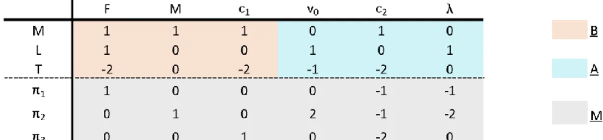
The technique used to compute the dimensionless products πi has been proposed by Langhaar
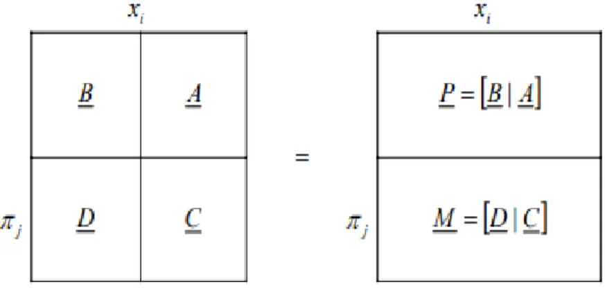
(1951). The first step of the procedure is setting up a matrix with a structure shown in Fig 5.
Figure 5 – Matrices for dimensionless numbers computation
The dimensional matrix P = [B | A] is composed of columns corresponding to the variables xi of the problem and by rows corresponding to the fundamental quantities. If the aim of the DA application is to relate a dependent variable x1 (target) to x2,..,xn independent variables as in
Eq. 1, the target x1 must be placed in the first column of P and the remaining variables should
be placed in a decreasing order of experimental control.
The element Pi,j (i = 1,..,n and j = 1,.., k) is the power coefficient of the j-th fundamental quantity describing the i-th dimensional variable.
The matrix P is a k x n matrix where k is equal to the number of fundamental quantities and n is equal to the number of initial variables. In case the rank of P resulted lower than k, it would be
38
possible to eliminate a row randomly, until the number of rows is equal to the rank r of the matrix. After that, the matrix P can be broken down into two sub-matrices:
● The square matrix A of dimension r × r; ● The sub-matrix B of dimension r × (n - r).
The sub-matrix D must be a square matrix of dimensions (n - r) x (n - r), chosen in order to create the dimensionless groups of the appropriate form. Generally, at first, the matrix D is set equal to the identity matrix. The approach proposed by Langhaar concludes with the computation of the sub-matrix C:
C=-D⋅ (A-1⋅ B)T
The dimensionless groups are obtained through the matrix M = [D | C], whose elements are the power of the respective variables in the dimensionless group πj. The dimensionless terms are computed using the following formula, where mij represents the element in matrix M.
𝜋𝑗 = ∏ 𝑥𝑖𝑚𝑖𝑗 𝑛
𝑖=1
Eq. 5
j = 1, …, n-r; i = 1, …, n
From an initial set of dimensional quantities, it is possible to derive different sets of dimensionless products. The theorem states that the πi terms belonging to the same set must be mutually independent. This means that any dimensionless product can be expressed as a product of powers of the remaining πj of the same set. The condition of independency of πi terms is a direct consequence of the independence of the dimensional variables xi.
As mentioned at the beginning of the current paragraph, the BT objective is the identification of a set of dimensionless numbers for which a functional relation F exists, so that Equation 2 is valid. Consequently, the following equation can be written:
𝜋1 = 𝐹′( 𝜋2, … , 𝜋𝑝),
39
If π1 has been correctly calculated, it must be the only one containing the dimensional target variable x1. Once function F’ has been experimentally or theoretically identified, the
dimensional target variable x1 is easily deduced.
1.2.3 Buckingham Theorem benefits
Reduction of the number of variables involved
The immediate result of the Dimensional Analysis application is the reduction of the number of variables describing the problem. This often leads to an enormous simplification of the necessary procedures in the analysis. In the work “The Physical basis of Dimensional Analysis” (Sonin, 2004), a practical case is described where one target variable and five independent variables are considered. The number of fundamental quantities is k=3. Therefore, Dimensional Analysis reduces the number of independent variables from five to two. Let us suppose that 10 experiments (data points) for each dimension (variable) of the research space are needed. Considering that the number of data points grows exponentially with the number of variables, 105 data points would be required to get the desired data density. Reducing the number of independent variables from 5 to 2, the required data points to get a comparable resolution is 102. Therefore, the number of experiments needed decreased by 99,9%.
Similarity
Another relevant contribution is the construction of models in scale. Scale modeling deals with the following question: ‘If we want to learn something about the performance of a full-scale
system 1 by testing a geometrically similar small-scale system model 2 at what conditions should we test the model? And how should we obtain the full-scale performance from measurements at the small scale?’ Dimensional Analysis provides the answer. Indeed, transforming the
dimensional variables into πi terms, we are able to make our analysis and tests on a reduced model. For instance, in presence of projects characterized by high costs, it is useful to study the results obtained on a reduced model, limiting in this way, the impact of each experimental trial and possible mistakes.
40
The concept underlying Similarity is that two distinct data points P1 and P2 in the dimensional space (n dimensions) might be represented by the same datapoint p1 in the dimensionless space (n-k dimensions). Therefore, collecting experimental data in conditions P1 is equivalent to collecting data in conditions P2. This is valid because the dimensionality reduction represents a surjective mapping function.
Higher domain knowledge
The application of the Buckingham Theorem is also an opportunity for the researcher to get insights on the general principles ruling the analyzed phenomenon. Thanks to the interpretation of the physical meaning of πi terms, some relations and dependencies between dimensional variables and target variable can be highlighted. A widely known dimensionless number is Reynolds Number 𝑅𝑒 =𝜌𝑣𝐷
𝜇 used in fluid dynamics to characterize the flow of a fluid. The relation expressed by Re points out that, given a specific fluid (𝜌; 𝜇), if the geometry (D) of a pipe is fixed, the flow typology only depends on the flow velocity (v).
1.2.4 An illustrative example
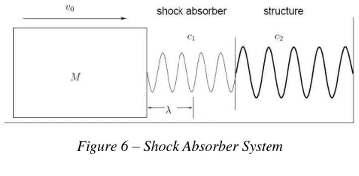
The following example from Rudolph (1998) of a Shock Absorber system for a moving mass
M with speed v0 in front of an immobile barrier, aims at providing a practical application of the BT.
By resorting to a traditional solving approach, i.e. relying on the laws of mechanics and dynamics, the following equation is found for F as a function of the considered variables:
𝐹 = √𝑐2𝑣02𝑀 − 𝜆2𝑐 2𝑐1
The objective is to show the reader how the key concepts of the theorem can be transferred to a real case.
41
A schematic representation of the system and the complete set of the n independent dimensional variables involved are shown respectively in Fig.6 and Fig.7.
The goal of the analysis is to estimate the maximum force F exchanged during an elastic collision between the mass M and the Shock Absorber.
The k fundamental quantities needed to describe the problem are: [M], [L] and [T]. All the dimensional variables can be expressed by products of powers of the fundamental quantities. The number of expected πi terms is p = n - k = 3. All the hypotheses previously listed for the
applicability of the theorem are satisfied. In fact, fundamental quantities are linear and additive quantities, the set of dimensional variables is complete and composed of independent variables. Therefore, it is possible to proceed with the computation of dimensionless terms.
Following the procedure described in paragraph 1.2.2, the matrices A, B, and M are computed (Table 5) and the three dimensionless numbers, presented below, are derived.
Figure 6 – Shock Absorber System