SCUOLA DI INGEGNERIA E ARCHITETTURA
DIPARTIMENTO DISI
CORSO DI LAUREA
IN
INGEGNERIA INFORMATICA
TESI DI LAUREA
In
Calcolatori Elettronici T
Evaluation of confidence-driven cost aggregation strategies
CANDIDATO:
RELATORE:
Matteo Olivi
Prof. Stefano Mattoccia
CORRELATORE:
Dott. Matteo Poggi
Anno Accademico 2015/2016
“Considerate la vostra semenza: fatti non foste a viver come bruti, ma per seguir virtute e canoscenza”
i
Ringraziamenti
La mia laurea, il primo traguardo della mia vita adulta, è arrivata. Non so perché quando ci pensavo pochi anni fa mi sembrava un evento indefinito collocato in un futuro lontano. E invece eccomi qua. Quindi, non posso non ringraziare le persone che hanno contribuito, in modo diretto e indiretto, a questo traguardo.
Comincio con il ringraziare il Prof. Stefano Mattoccia per avermi dato la possibilità di approfondire un campo di ricerca così interessante come quello della Stereo Vision. E’ stata la mia prima opportunità di studiare qualcosa in modo approfondito e sarà sempre un bel ricordo. Un ringraziamento sentito va anche al Dott. Matteo Poggi per l’aiuto, la pazienza e il tempo che mi ha dedicato.
Un enorme grazie a mio padre, per avermi sempre sostenuto e incoraggiato nei momenti difficili, e gioito con me nei momenti più belli. Grazie anche a Caterina che a cena ascolta tutto quello che dico con interesse, anche se magari è stanca e vorrebbe solo mangiare. Grazie a Marco e Tersea, che anche se ci si vede poco fa sempre piacere. Un grandissimo grazie anche a tutti i miei parenti per l’affetto con cui mi accogliete ogni volta che ci vediamo e per la fiducia che avete in me.
Grazie a Dave e Garro, che ci sono da sempre. Incredibile , 16 anni e ancora amici. Semplicemente fantastico. Grazie anche alla Brianza Alcolica per il tempo passato assieme, che ogni tanto bisogna anche rilassarsi.
Un grazie speciale va anche a Steve. Siamo entrati assieme, usciremo assieme. Sono contento di aver fatto questi tre(due) anni di Università con te. Grazie anche ai Ciao cari e agli altri compagni dell’Università per aver reso questi tre anni molto più divertenti. Infine, grazie ai compagni del liceo, che anche se io non ci sono quasi mai sono sempre felici di vedermi.
ii
Introduction
Stereo Vision is the subfield of Computer Vision whose aim is to infer the 3D coordinates of a scene starting from two pictures of that scene taken from two different positions.
A lot of research on this topic is being carried out because of its many applications: self-driving cars, robots, drones and others. Basically everywhere there is a system that needs to move autonomously (i.e. without a human being driving it, either remotely or in place), Stereo Vision is needed.
The reason for this is that the first step for the system to be able to choose where to go and how to move is knowing its surroundings. For instance, if an autonomous car has an obstacle right in front of it and must therefore dodge it, it must first detect the object, and know its location and shape as precisely as possible.
The latter example introduces why we are not satisfied with the Stereo Vision algorithms we currently have. They need to be fast, because they are to be used in real time applications. And they need to be accurate.
State-of-the-art Stereo Vision algorithms do not yet meet a reasonable trade-off between these two conflicting requirements. This thesis is an attempt to perform a little step forward to produce more accurate algorithms.
To do that, I tried to use a Guided Filter with a Confidence Map as a guide. Chapters 1 to 3 are the introductive chapters and present the notions needed to understand the research work I have done. More specifically, Chapter 1 is an overview of Stereo Vision (especially Stereo Matching). Chapter 2 is a brief explanation of what a Guided Filter is, while Chapter 3 presents the concepts of Confidence and Confidence Map. Chapter 4 explains in detail what I have done. Chapter 5 shows the highlights of the experimental results. Finally, Chapter 6 presents the Conclusions of this thesis.
iii
Table of Contents
Ringraziamenti ... i
Introduction ... ii
Table of Contents ... iii
Table of Figures ... v
Table of Tables ... vii
Chapter 1. Stereo Vision ... 1
1.1 Problem definition ... 1
1.2 Stereo matching ... 2
1.2.1 Problem definition ... 2
1.2.2 The epipolar constraint ... 3
1.2.3 Disparity map ... 4
1.2.4 How to compute disparity ... 5
1.2.5 Disparity space image(DSI) ... 5
1.2.6 Cost aggregation ... 6
1.3 Depth from Triangulation ... 9
Chapter 2. Guided Filtering ... 10
2.1 Guided filter... 10
Chapter 3. Confidence measures ... 12
3.1 Confidence and Confidence map ... 12
3.2 PKR and PKRN confidence measures ... 13
3.2.1 PKR Confidence ... 13
3.2.2 PKRN Confidence ... 15
Chapter 4. Proposed algorithms ... 16
4.1 The general idea ... 16
4.2 Algorithms description ... 17
4.2.1 PKRN ... 18
4.2.2 PKRN + left ... 19
4.2.3 left + PKRN ... 19
4.2.4 left + PKRN downstream... 20
Chapter 5. Experimental results ... 22
5.1 Preliminary considerations ... 22
5.2 Aggregated results ... 24
5.3 Picture by picture results ... 25
5.3.1 Tsukuba ... 25
iv
5.3.3 Cones ... 30
5.3.4 Venus ... 32
5.4 Observations on the results ... 34
5.5 The negative costs problem ... 36
Chapter 6. Conclusions and future work... 37
v
Table of figures
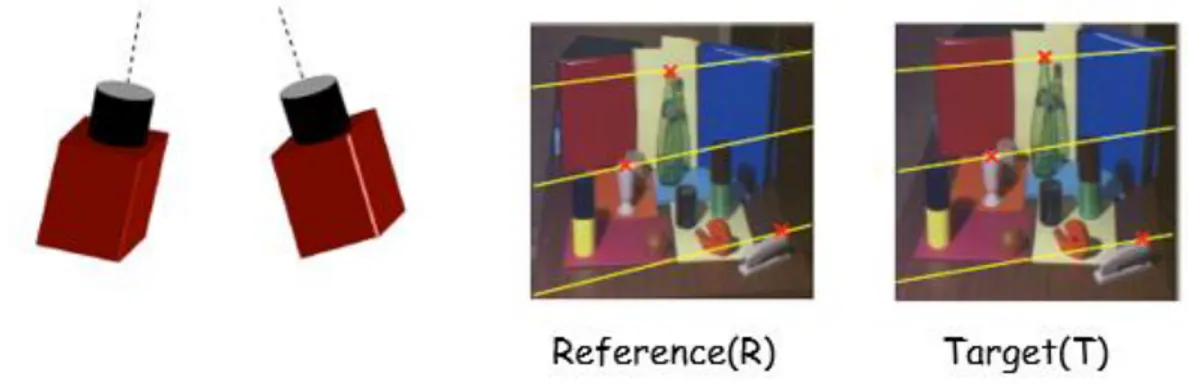
Fig. 1.1: Stereo pair of cameras and Reference and Target images with corresponding points highlighted
(red dots). ... 1
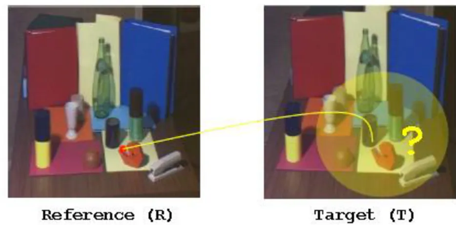
Fig. 1.2: The point in T corresponding to the red point in R must be found. ... 2
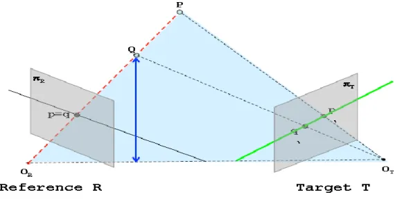
Fig. 1.3: The red dashed line represents a Line of Sight of the left camera. All the points belonging to it are projected onto the same point on reference picture R and the same line on the target picture T ... 3
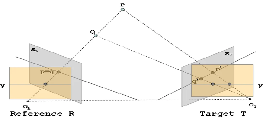
Fig. 1.4: With the Stereo Rig in Standard Form the points in R will have the same y coordinate of the corresponding point in T. ... 4
Fig. 1.5: A Stereo pair R (top-left) and T (top-right), with their disparity map (bottom)... 5
Fig. 1.6: A DSI. The element of coordinates (x,y,d) is the cost for assigning disparity d to the pixel of coordinates (x,y) of the Reference Image. ... 6
Fig. 1.7 : Groundtruth (i.e. ideal) disparity map(left) and disparity map obtained through eq. 1 (right)... 7
Fig. 1.8: : Aggregation window S on reference image and corresponding aggregation window on target image. The red dot in the left image is p(x,y), while the red dot in the right image is the pixel of coordinates (x+d,y). ... 8
Fig. 1.9: OR and OT are the optical centers of reference and target respectively. f is the focal distance of the stereo pair cameras. P is the point whose depth is being computed. p and p’ are the projections of P on reference and target respectively. xR and xT are the x coordinates of p and p’. Z is the depth to compute. B is the distance between the optical centers of the two cameras. ... 9
Fig. 3.1: Two disparity maps (upper row), and their confidence maps (lower row).. ... 13
Fig. 3.2: Cost curve (a) is ideal because there is only one local minimum and it is much smaller than all the other costs. Cost curve (b) is more ambiguous: there are three local minimum and they have relatively similar values... 14
Fig. 3.3: A cost-over-disparity curve. Note that there is only one local minimum. ... 15
Fig. 4.1: Schema of the algorithms proposed by Rhemann et al. in [6] and De-Maetzu et al. [1] ... 16
Fig. 4.2: “PKRN” algorithm pipeline schema ... 18
Fig. 4.3: “PKRN + left” algorithm pipeline schema ... 19
Fig. 4.4: “left + PKRN” algorithm pipeline schema ... 20
Fig. 4.5: “left + PKRN Downstream” algorithm pipeline schema. ... 21
Fig. 5.1: The four stereo pairs from the Middlebury stereo benchmark I tested the algorithms with. Starting from the top-left corner, going clockwise: Tsukuba, Cones, Teddy, Venus ... 22
Fig. 5.2: Groundtruth disparity maps for the four stereo pairs from the Middlebury Stereo benchmark, from the top-left corner, going clockwise: Tsukuba, Cones, Teddy, Venus. ... 23
Fig. 5.3: From top-left picture, going clockwise: Original (FCVF) disparity map, left + PKRN downstream disparity map, groundtruth disparity map. ... 27
Fig. 5.4: : From the top-left picture, going clockwise: Original (FCVF) disparity map, PKR disparity map, groundtruth disparity map ... 27
Fig. 5.5: From top-left picture, going clockwise: Original (FCVF) disparity map, PKRN + left disparity map, groundtruth disparity map. ... 29
vi
Fig. 5.6: From the top-left picture, going clockwise: Original (FCVF) disparity map, left + PKR downstream map, groundtruth map. ... 29 Fig. 5.7: From the top-left picture, going clockwise: Original (FCVF) disparity map, left + PKRN downstream map, groundtruth map. ... 31 Fig. 5.8: From the top-left picture, going clockwise: Original (FCVF) disparity map, PKRN disparity map, groundtruth map. ... 31 Fig. 5.9: From the top-left picture, going clockwise: Original(FCVF) disparity map, PKR + left downstream map, groundtruth map... 33 Fig. 5.10: From the top-left picture, going clockwise: Original (FCVF) disparity map, left + PKR downstream map, groundtruth map. ... 33 Fig. 5.11: A sparse confidence map(left) and a dense confidence map(right) ... 36
vii
Table of tables
Table 5.1: Ranking of the algorithms by average % error and threshold = 3. The FCVF algorithm as proposed
in [6] is in boldface... 24
Table 5.2: Algorithms ranked by average percent error reduction with respect to the FCVF algorithm as proposed in [6]. The algorithms that achieved an improvement are characterized by a positive value in the central column. Those that did worse than the original are characterized by a negative value in the central column. ... 25
Table 5.3: Algorithms ranked by percent error with threshold at 3 for Tsukuba ... 26
Table 5.4: Algorithms ranked by percent error with threshold at 3 for Teddy ... 28
Table 5.5: Algorithms ranked by percent error with threshold at 3 for Cones ... 30
Table 5.6: Algorithms ranked by percent error with threshold at 3 for Venus ... 32
Table 5.7: For every algorithm, the number of first placements, last placements and improvements with respect to FCVF across all the individual rankings is shown. Note that the sum over the first two columns (first and last placements) is bigger than 4 as there are some ties. ... 35
Table 5.8: The total number of first placement, total number of last placements, and total number of improvements across all the individual rankings for PKRN and PKR algorithms. ... 35
Table 5.9: The total number of first placement, total number of last placements, and total number of improvements across all the individual rankings for algorithms that perform a double smoothing and all the others ... 35
1
Chapter 1. Stereo Vision
This chapter provides the theoretical framework to be able to understand this thesis work. It explains what Stereo Vision is, what is its goal and what are the techniques that belong to this field. It comprises all the foundations of Stereo Vision, ranging from Computer Vision notions to physical and optical laws.
1.1
Problem definition
As stated in the Introduction, the problem Stereo Vision aims to solve is: Given two (or more) images of the same scene taken at the same time from two cameras placed at different positions, infer the depth (as well as the other coordinates) of all the points that appear in both images. The solution to this problem is split into two parts:
1. Choose one picture as the reference (typically the leftmost one), and for every point in it find the corresponding point in the other image (target image): This problem is called Stereo Matching.
2. With the information obtained at 1., use triangulation to compute the depth of all the points.
Fig. 1.1 Stereo pair of cameras and Reference and Target images with corresponding points highlighted (red dots).
Fig 1.1. shows a stereo rig (the pair of cameras), and the two pictures of the same scene. Corresponding points across the two images are signed as red dots. Between the two aforementioned steps, 2. is rather simple and straightforward, while stereo matching is the most challenging one and is where all the research is being done.
2
1.2 Stereo matching
1.2.1 Problem definition
Consider a reference picture R and another picture, which we will call target T, of the same scene taken at the same time but from a different position. Now take a point p belonging to R. Stereo matching is the problem of finding where p ended up in T, that is to say, the point p’ in T that corresponds to p. What I mean by “corresponds” is that the two points p and p’ in R and T respectively, represent the same point of the scene being photographed. This step is shown in Fig. 1.2 where we have the left picture being the reference R, the right one being the target T, and for the red point in R we have to find the corresponding point in T.
Fig. 1.2 The point in T corresponding to the red point in R must be found.
As we are working with digital images, the points I mentioned in the previous paragraph will be pixels. In this context, stereo matching can be reformulated as: given the pixel p of coordinates (x,y) in R, find d_x and d_y such that the pixel p’ of coordinates (x + d_x, y + d_y) in T corresponds to p.
3
1.2.2 The epipolar constraint
Considering what we have said this far, stereo matching appears to be a 2D search problem, because we have to determine both d_x and d_y, or, alternatively, both coordinates of pixel p’ in T.
Fortunately, we can simplify it to a 1D search problem thanks to the epipolar constraint: All the points belonging to the same line of sight of image R (red dashed line in Fig. 1.3) will be projected onto to the same line in T (green continuous line in Fig.1.3).
Fig. 1.3 The red dashed line represents a Line of Sight of the left camera. All the points belonging to it are projected onto the same point on reference picture R and the same line on the target picture T.
A consequence of the epipolar constraint is that there is always a setup of the stereo rig (i.e. the pair of cameras), called standard form, such that a pixel p in R will have the same y coordinate as pixel p’ in T (See Fig. 1.4 on next page).
The standard form of the stereo rig is impossible to achieve physically, because this would require calibration techniques that are more precise than what we can do. But, starting from a pair of pictures taken from a rig in non-standard form, we can apply a transformation and obtain the pictures that would have been taken if the rig had been in standard form.
Once we have the two images in standard form, stereo matching becomes a 1D problem, because we do not have to search for d_y, as it will always be d_y = 0. Now we only have to find the d_x such that pixel p(x,y) in R corresponds to pixel p’(x + d_x,y) in T. Because
4
of the lack of ambiguity that this simplification yields, we will start calling d_x d instead. The technical name for d is disparity.
Fig. 1.4 With the Stereo Rig in Standard Form the points in R will have the same y coordinate of the corresponding points in T.
1.2.3 Disparity map
So far we have been discussing the problem of how to compute a single pixel p depth. In order to do that we first have to compute its disparity d. As our final goal is to compute the depth of all the points of the scene being acquired with the two cameras, we must compute the disparity d for every pixel in the reference image R.
Thus, given a stereo pair of pictures R and T, we can define its disparity map as a function that assigns to every pixel p of R its disparity d. Conveniently for us, we can represent a disparity map Dm as a grayscale image. The intensity value of the pixel of coordinates (x,y) in Dm is proportional to the disparity value d of the pixel of coordinates (x,y) in R.
The advantage of this representation is that it makes a first-order evaluation of the disparity map quick and intuitive for a human being. A disparity map is shown in Fig. 1.5.
5
Fig. 1.5 A stereo pair R (top-left) and T (top-right), with their disparity map (bottom).
1.2.4 How to compute disparity
In all the previous paragraphs, we haven’t explained yet how we can actually compute disparity, that is to say, how we can build a disparity map. We will do it now.
According to [7] and [9], all the stereo matching algorithms fall into two classes: local methods and global methods. Global methods perform the disparity assignment of all the pixels in the reference image R simultaneously, by looking for the overall assignment that minimizes a certain energy function. They are very accurate but very time consuming. We will not talk about them anymore, as they are out of the scope of this thesis, which treats only local stereo matching algorithms.
Local methods assign disparity to one pixel p at the time, and they make use of information about the pixels neighboring p. They choose the disparity d among a set of possible values by looking for the one which minimizes a given cost function.
1.2.5 Disparity space image (DSI)
Usually, in the context of stereo matching we can assume that disparity will always be within a given range dmin, …, dmax,called Horopter,where dmin and dmax are both known. Their actual
6
values will depend on the particular application, and for the sake of simplicity we will from now on assume dmin = 0 (as a matter of fact, it is often true).
Every local stereo matching algorithm follows, more or less, the same pattern: for every pixel p in the reference picture R, it considers all the possible disparity assignments 0, …, dmax. Then, for every possible assignment d, it computes the value of a given function called
cost function (this value is the cost for assigning disparity d to pixel p). Consequently, we can define a 3D matrix called disparity space image(DSI) where the element (x,y,d) is the cost for assigning disparity d to the pixel of the reference image R of coordinates (x,y). The disparity map is then built by analyzing the DSI and assigning to every pixel the disparity d with minimum cost (it’s rare, but some algorithms choose the disparity with the maximum cost when a similarity function is adopted). This approach is called Winner-Takes-All(WTA) selection. Fig. 1.6 shows an example of DSI.
Fig. 1.6A DSI. The element of coordinates (x,y,d) is the cost for assigning disparity d to the pixel of coordinates (x,y) of the Reference image.
1.2.6 Cost aggregation
The most intuitive and naïve cost function is the absolute difference of the intensity values of the two pixels of coordinates (x,y) and (x + d, y) in R and T respectively:
7
This cost function produces very noisy results (see Fig. 1.7), thus something better is needed. A very popular approach which has emerged consists of aggregating costs near the pixel whose cost is being computed.
To put it in simpler words, it means that the cost for assigning disparity d to pixel p of coordinates (x,y) in R no longer depends only on p itself and the pixel of coordinates (x+d,y) in T(that’s the case of eq. (1)), but also on the pixels neighboring them.
Fig. 1.7 Groundtruth (i.e. ideal) disparity map(left) and disparity map obtained through eq. 1 (right).
For instance, Fixed Window + SAD (Sum of Absolute Differences), is an algorithm that implements this idea. It builds a DSI where the costs are computed with eq. (1). Then, for every pixel p in R it considers a squared window S of fixed size centered on p. At this point it substitutes to every element of the DSI the sum of the costs (for the same disparity
assignment d) of the pixels belonging to S. Thus, the cost function becomes:
(2)
where (x,y) are the coordinates of the pixel p of R whose costs are being computed, d is the disparity assignment for which the cost is being computed, S is the squared window
8
Fig. 1.8 Aggregation window S on reference image and corresponding aggregation window on target image. The red dot in the left image is p(x,y), while the red dot in the right image is the pixel of coordinates (x+d,y).
While this algorithm is an improvement with respect to the first one, it still produces inaccurate results. As a consequence, some variations that use the same idea were proposed, such as one where the window S no longer has to be centered on p, another one where the size of S is variable, a combination of the aforementioned two, and many others. Another popular approach is to weight the contribute of each pixel in the aggregation window with the probability of it belonging to the same object as the pixel p (whose costs are being computed). [11] is a thorough survey of the cost aggregation methods that have been developed.
9
1.3 Depth from Triangulation
Once we have inferred the disparity of a pixel in the reference image, we can compute its depth, by means of the triangulation:
Fig. 1.9 OR and OT are the optical centers of reference and target respectively. f is the focal distance
of the stereo pair cameras. P is the point whose depth is being computed. p and p’ are the
projections of P on reference and target respectively. xR and xT are the x coordinates of p and p’. Z is
the depth to compute. B is the distance between the optical centers of the two cameras.
With respect to Fig. 1.9, we have:
(3) (4) Thus: (5) (6) (7)
10
Chapter 2. Guided Filtering
This brief chapter introduces the broad ideas underpinning the Guided Filter operation. While a high-level understanding of this type of filter is necessary to understand this thesis work, the details are not, hence they are not presented. If you wish to have a deeper knowledge on this topic, you can read [2].
2.1
Guided Filter
In [2] a new image filter was proposed. Its purpose was to serve as an edge-preserving smoothing filter, making it suited for noise reduction.
It was called guided filter as the value of the pixels of the output image (i.e. filtered image) depends on the values of the pixels of a second input image. From a high-level perspective, the second image, called guidance, is “guiding” the filtering/smoothing process, hence the name.
Going a little bit more into details, the guided filter was inspired by the idea that the output pixel qi of coordinates (x,y) should be a weighted average of the pixels from the input
image in a squared window centered at (x,y):
(10)
where i and j are pixel indexes, I is the guidance image, p is the input image, and Wij
depends on I and is independent of p. This is not a new idea as there are many filters that use it, such as the bilateral filter ([10]).
Another key assumption in the development of this filter was the local-linearity between the guidance image I and the output q. The idea is that q is a linear model of I in a window wk
centered at pixel k:
(11)
11
Note that a property of such a filter is that q has an edge only if I has an edge, because . Hence the edge-preserving property. For the sake of honesty, this is not exactly how a guided filter works and these properties are slightly different from the ones a guided filter actually has, but for the scope of this thesis it suffices to know about the local-linearity property, and that the actual behavior of the guided filter was derived starting from the features and formulas above.
Also, note that these types of filters applications go beyond image smoothing, as they can also be successfully used for image matting ([4]) and haze-removal ([3]).
Finally, one last thing worth mentioning is that, unlike many similar filters (such as the one proposed in [10]), the run-time of the guided filter does not depend on the radius of the window used to compute the weighted average of pixels (wk in (11)), but only on the size of
the input images (there being the constraint of them having the same size). This yields a very low runtime for the guided filter when compared against the one of other filters alike, especially when the size of the image to filter grows, as this requires the radius of the aggregating window to grow too.
12
Chapter 3. Confidence measures
This chapter explains the concept of Confidence, the last piece needed to understand this research. It starts by giving a general overview of Confidence, and then the focus moves on the aspects that are more closely related to this thesis.
3.1
Confidence and Confidence map
In Chapter 1 we explained what a disparity map is and that it is the output of stereo matching algorithms. As there are different stereo matching algorithms and different cost functions, for the same input stereo pair different algorithms will produce different disparity maps. Since there is the need to understand how good a disparity map is, a measure of their quality was introduced: confidence.
With respect to a pixel p(x,y) of a disparity map, its confidence is a measure of “how confident” we are about the fact that its value(i.e. the disparity of the pixel of coordinates (x,y) in R) is correct(or close to correctness).
If we have a disparity map D, we can compute the confidence value of every pixel. Therefore, just like we did for disparity maps, if we consider the function that assigns to every pixel of D its confidence value, we can represent this function as a grayscale image where the value of the pixel of coordinates (x,y) is proportional to the confidence value of pixel (x,y) of D. For completeness, Fig. 3.1 shows two disparity maps with their corresponding confidence maps. As a rule of thumb to interpret them, the darker the pixel, the lower the confidence.
13
Fig. 3.1 Two disparity maps (upper row), and their confidence maps (lower row).
3.2
PKR and PKRN confidence measures
As for how to compute confidence, there are many different measures.
[5] is a thorough study of most of the confidence measures that have been proposed so far, and provides some experimental results to evaluate and rank them.
As this thesis is an attempt to use confidence to produce good-quality disparity maps, a choice had to be made on which measures to use. The choice has fallen on PKR(Peak Ratio) and PKRN(Peak Ratio Naive) confidence, as they are very simple to implement and ranked among the bests according to [5].
Both measures take as input the DSI from which the disparity map was produced (with WTA selection), and consider the cost-over-disparity curve for a pixel to compute its confidence. The underlying assumption is that a disparity assignment d is a good candidate if its cost is small and if the costs decrease as disparity gets closer to d (that is to say, the cost of d is a local minimum). The next two sections explain PKR and PKRN confidence.
3.2.1
PKR ConfidenceAs stated above, PKR stands for Peak Ratio. Consider a DSI and a pixel of coordinates (x,y). Now consider the column of the DSI with the costs for (x,y). Let c1 and c2m be the minimum
cost and the second smallest local minimum of the cost-over-disparity curve respectively. Then the confidence of pixel (x,y) is defined as:
14
(8)
To understand what is the idea behind this measure, let’s consider two different cost curves, in Fig. 3.2(taken from [5]) on the next page. Let’s begin with curve (a): There is only one local minimum, and all the other costs are much bigger. Consequently, the resulting PKR confidence value will be big. This is good, because since there is only one minimum which is considerably smaller than all the other costs, we are quite confident that the right disparity is the one at which the minimum occurs.
On the other hand, if we consider curve (b) we see that besides the minimum c1 there is
another local minimum c2m that is close to it.Thus, the PKR confidence value will be small.
Once again, this is what we want, because even if the disparity that will be chosen is the one at which the minimum c1 occurs (by virtue of the WTA selection), there was another disparity
which yielded a good cost(c2m).
Fig. 3.2 Cost curve (a) is ideal because there is only one local minimum and it is much smaller than all the other costs. Cost curve (b) is more ambiguous: there are three local minimum and they have relatively similar values.
15
3.2.2 PKRN Confidence
PKRN stands for Peak Ratio Naïve, and it is a simplified and less accurate version of the PKR confidence. The formula is the same as the one for PKR, but instead of the second smallest local minimum of the cost-over-disparity curve the second smallest cost is used at the numerator. With respect to Fig. 3.2, if we compute the PKRN confidence for cost curve (b), we have:
(9)
Why is this measure less accurate? Becausethe disparity at which c2 occurs might not be
a good candidate, as it might be next to a disparity with a smaller cost. To better understand this, consider the cost curve in Fig. 3.3.
As the curve is strictly increasing, the confidence should be really high, since there is only one strong candidate, that is, d = 1. But if we were to use the PKRN measure, a low confidence value would be computed as c2 is very close to c1.
Interestingly enough, despite these arguments, both my experimental results and those in [5] suggest that PKRN produces more accurate results than PKR.
16
Chapter 4. Proposed algorithms
As mentioned in the Introduction, the goal of this thesis is to propose new Stereo Matching algorithms that achieve better accuracy than current ones by using confidence. This chapter describes the proposed algorithms. There are eight, and they are all very similar because they are based on the same idea: smoothing a DSI with a guided filter using a confidence map as the guidance image.
4.1
The general idea
Both Rhemann et al. in [6] and De-Maeztu et al. in [1] described a new stereo matching algorithm that made use of a guided filter. The algorithm in [1] was called “Linear Stereo matching”, while the authors of [6] called their “Fast Cost-Volume Filtering”, and from now on I will refer to it with the acronym of FCVF. Their idea was to build a DSI with punctual costs (albeit a variation with respect to the one described by eq. (1) on page 8), and then smooth every slice of the DSI where d is constant with a guided filter, using the Reference image (left) of the stereo pair itself as the guide. Then they chose the disparity assignments with a WTA selection. Fig. 4.1 is a schema of this algorithm.
Fig. 4.1 Schema of the algorithms proposed by Rhemann et al. in [6] and De-Maetzu et al. [1]
The initial idea for this thesis was to do exactly what they had done, but using a confidence map as the guidance image of the guided filter. As their algorithm has a pipeline-like structure, fostering the addition of other filtering stages upstream or downstream the central one (i.e. DSI smoothing with left image as a guide), we also thought about some other modifications, such as smoothing the DSI twice, once with confidence and once with
17
the reference(left) image, both in this order and the opposite one. Another experiment we tried was the use confidence to smooth a disparity map itself rather than the DSI it was built from.
Finally note that the algorithms proposed in [6] and [1] made use of a left-right consistency check, a downstream pipeline stage used to exclude occluded pixels (those that appear only on one of the images of the stereo pair) from the final disparity map (see [6] and [1] for details). For the sake of simplicity, we chose not to do that in the proposed algorithms, as it requires, without deploying algorithmic manipulation to the DSI, to execute every step of the algorithm twice, once using the left image as the reference, then using the right image, and finally comparing the two disparity maps against each other (this means that the runtime is increased up to twice as long as the “normal algorithm”).
A consequence of this choice is that when in Ch. 5 we compare the results of the proposed algorithms with the ones of the original algorithm (linear stereo in [1], FCVF in [6]), in particular the latter is a modified version of the one proposed in [6], the only difference being that there is no left-right consistency check.
4.2
Algorithms description
Each one of the following sections describes one of the algorithms proposed in this thesis. For every one of them there is also a schema similar to the one on Fig. 4.1. Each section name is the abbreviated name used to reference the corresponding algorithm in Chapter 5 where the experimental results are presented. Note that only four algorithms are shown, and that they all make use of the PKRN confidence measure. For every one of them, there is also an absolutely identical algorithm that makes use of the PKR confidence measure instead. In all the following algorithms, when I say “build punctual DSI” the said DSI is built in the same way as the one in the original algorithm proposed in [6] and [1].
As all the algorithms involve at least one smoothing of a DSI with a guided filter, the name of the algorithm represents what is used as the guidance image for the smoothing. For instance, if the name of the algorithm is “PKRN”, it means the smoothing is performed using a PKRN confidence map as the guidance image.
If the DSI is smoothed twice, the name of the algorithm will comprise both guidance images (in the same order they are used). For example, if the name is “PKRN + left” it means
18
that the first smoothing is performed with a PKRN confidence map while the second one with the left image.
Finally, if a smoothing is performed on a disparity map instead of a DSI, what was used as the guidance image will appear in the algorithm name followed by the word “downstream” (e.g. PKRN downstream).
Note that the names in the following sections are the names used in Chapter 5 to reference the algorithms when presenting the experimental results.
4.2.1 PKRN
This algorithm is the same as the FCFV ([6]), but a PKRN confidence map is used to smooth the DSI instead of the reference image.
Algorithm reference name in Ch. 5: PKRN.
Equivalent PKR algorithm reference name in Ch. 5: PKR. The steps for this algorithm are:
1. Build punctual DSI.
2. Compute the PKRN(PKR) confidence map from the DSI.
3. Smooth the DSI slices where d is constant with a guided filter using the PKRN(PKR) confidence map as the guidance image.
4. Build the disparity map with a WTA selection on the smoothed DSI.
19
4.2.2 PKRN + left
In this algorithm a punctual DSI is built and then is smoothed twice: first with its PKRN confidence map, then with the reference(left) image.
Algorithm reference name in Ch. 5: PKRN + left.
Equivalent PKR algorithm reference name in Ch. 5: PKR + left. The steps for this algorithm are:
1. Build punctual DSI.
2. Compute the PKRN(PKR) confidence map from the DSI.
3. Smooth the DSI slices where d is constant with a guided filter using the PKRN(PKR) confidence map as the guidance image.
4. Smooth the DSI (obtained from 3.) slices where d is constant with a guided filter using the reference(left) image as a guide.
5. Build the disparity map with a WTA selection on the DSI obtained from the previous step.
Fig. 4.3 “PKRN + left” algorithm pipeline schema.
4.2.3 left + PKRN
This algorithm is similar to “PKRN + left”, but the order of the two smoothing stages is reversed: the first smoothing is performed with the reference(left) image as the guidance image, while the second one uses a PKRN(PKR) confidence map.
Algorithm reference name in Ch. 5: left + PKRN.
Equivalent PKR algorithm reference name in Ch. 5: left + PKR. The steps for this algorithm are:
20
2. Smooth the DSI slices where d is constant with a guided filter using the reference(left) image as the guidance image.
3. Use the DSI obtained from 2. to compute a PKRN(PKR) confidence map.
4. Smooth the DSI slices where d is constant with a guided filter using the PKRN(PKR) confidence map as the guidance image.
5. Build the disparity map with a WTA selection on the DSI obtained from the previous step.
Fig. 4.4 “left + PKRN” algorithm pipeline schema.
4.2.4 left + PKRN downstream
This algorithm is different with respect to the previous ones, as one smoothing is performed on a disparity map instead of the DSI. It consists of building a punctual DSI, smoothing it with the reference(left) image, then using it (the smoothed DSI) to compute both a PKRN(PKR) confidence map and a disparity map (with WTA selection), and filtering the latter disparity map with the confidence map.
Algorithm reference name in Ch. 5: left + PKRN downstream.
Equivalent PKR algorithm reference name in Ch. 5: left + PKR downstream. The steps for this algorithm are:
1. Build punctual DSI (in the same way as the original algorithm).
2. Smooth the DSI slices where d is constant with a guided filter using the reference(left) image as the guidance image.
3. Use the DSI obtained from 2. to compute a PKRN(PKR) confidence map.
21
5. Smooth the disparity map obtained from 4. with a guided filter and the PKRN(PKR) confidence map obtained from 3. as the guidance image.
22
Chapter 5. Experimental results
In this chapter, we present the experimental results of the execution of
the proposed algorithms on four stereo pairs from the Middlebury Stereo benchmark [8]. The data is presented both in aggregated form (i.e. averages) and for every single picture.
5.1
Preliminary considerations
In [6], the authors made available a Matlab implementation of the proposed algorithm and a demo with four Stereo pairs from the Middlebury Stereo benchmark [8]: Tsukuba, Teddy, Cones and Venus.
As the algorithms in this thesis are built on top of the algorithm in [6], it came as a natural choice to test them on the very same stereo pairs, to facilitate the comparison of the results between the original and the modifications. In Fig. 5.1 the four stereo pairs are shown.
Fig. 5.1The four stereo pairs from the Middlebury stereo benchmark I tested the algorithms with. Starting from the top-left corner, going clockwise: Tsukuba, Cones, Teddy, Venus.
As for the language to implement them with, the choice fell on Matlab, because of its high abstraction and wide range of predefined high-level image processing functions. This made the implementation process faster and simpler with respect to other languages, such
23
as C/C++. One drawback of this choice was that it made an analysis of the runtime of the algorithms impossible, because Matlab is very slow by nature, and the same algorithm implemented in C/C++ would run much faster. Thus, this work focus is on the accuracy of the results, not the runtime of the algorithms that yielded those results.
To compare and analyze the results, we made use of the groundtruth disparity maps for the four stereo pairs. A groundtruth disparity map is an almost perfect disparity map, obtained through the usage of structured light patterns. Fig. 5.2 shows the four groundtruth disparity maps.
Fig. 5.2 Groundtruth disparity maps for the four stereo pairs from the Middlebury Stereo benchmark, from the top-left corner, going clockwise: Tsukuba, Cones, Teddy, Venus.
Section 5.2 presents the aggregated data(averages) on the four stereo pairs. Section 5.3 presents the results separately for every stereo pair. In both sections, the algorithms are referenced with the names defined in Chapter 4, while the original algorithm ([6] and [1]) is referenced as “FCVF”. Section 5.4 contains some observations on the experimental results.
24
5.2
Aggregated results
Table 5.1 reports the ranking of the algorithms (with names as defined in Ch. 4) according to the average (considering all of the four stereo pairs) percent error of the disparity map they produce, with respect to the corresponding groundtruth map.
We chose to count a pixel disparity as an error if its distance from the corresponding groundtruth disparity is bigger than 3. The choice of this threshold against more intuitive values (such as 0) is a standard in literature, and it is due to the fact that even groundtruth values might not be 100% accurate and usually have an uncertainty of value 3. The algorithms are ranked from the best(top) to the worst(bottom), and the original FCVF algorithm (as proposed in [6]) is in boldface to make clear which algorithms are an improvement and which are retrogressions.
Algorithm name Avg. err %,
thresh. = 3 Rank left + PKRN 18.91 1 left + PKR 19.1425 2 PKR + left 19.45 3 PKRN + left 19.4525 4 FCVF 19.785 5 left + PKRN down 20.2875 6 PKRN 20.7275 7 PKR 20.7325 8 left + PKR down 20.7725 9
Table 5.1 Ranking of the algorithms by average % error and threshold = 3. The FCVF algorithm as proposed in [6] is in boldface.
What stands out the most from Table 5.1 is that all the algorithms that perform a double smoothing of the DSI rank better than the original, while all the algorithms that smooth the DSI only once rank worse than the original. This is even clearer from Table 5.2, that shows the average percent error reduction with respect to the percent error of FCVF. As we can see all the algorithms that smooth the DSI twice are characterized by a reduction of the average
25
percent error, while the other algorithms increase it.
Finally, both the best average percent error reduction (left + PKRN) and the worst average percent error increase (left + PKR downstream) are smaller than 1%, with 0.875% and -0.9875 % respectively. Thus, even if there has been an improvement, it is relatively small.
Algorithm name Avg. err. reduction %,
thresh. = 3 Rank left + PKRN 0.875 1 left + PKR 0.6425 2 PKR + left 0.335 3 PKRN + left 0.3325 4 left + PKRN down -0.5025 5 PKRN -0.9425 6 PKR -0.9475 7 left + PKR down -0.9875 8
Table 5.2 Algorithms ranked by average percent error reduction with respect to the FCVF algorithm as proposed in [6]. The algorithms that achieved an improvement are characterized by a positive value in the central column. Those that did worse than the original are characterized by a negative value in the central column.
5.3
Picture by picture results
Each one of the following sections presents the ranking with the same criteria as Table 5.1, but for only one of the four stereo pairs used in the experiments.
As a note about the notation used, when I use the expression “algorithms couple”, I mean two algorithms identical in everything but the confidence measure they use.
5.3.1 Tsukuba
Table 5.3 reports the ranking of the algorithms according to the percent error with threshold 3 on the Tsukuba disparity map. As the groundtruth Tsukuba disparity map has an all-zero padding near the boundaries, visible as a black frame (see Fig. 5.2 or Fig. 5.3), the comparison has been performed without considering those pixels.
26
Another interesting property is that the ranking is affected by the algorithm structure rather than the confidence measure used. What I mean is that it is possible to define a ranking between the algorithms couples. Alternatively, if an algorithm A that makes use of the PKRN(PKR) confidence does better than another algorithm B with the PKRN(PKR) confidence, the algorithm A’ identical to A except for the fact that it uses the PKR confidence does better than B too. The vice versa is also true.
Algorithm name % err Rank
left + PKRN down 2.43 1 FCVF 2.78 2 left + PKR down 2,83 3 left + PKRN 2.91 4 left + PKR 3.22 5 PKR + left 5.54 6 PKRN + left 5.55 7 PKRN 6.51 8 PKR 6.51 8
Table 5.3 Algorithms ranked by percent error with threshold at 3 for Tsukuba.
To have an idea of what these results mean, let’s consider the best disparity map, which is produced by the left + PKRN downstream, in Fig. 5.3. We can see that from a first look the original(FCVF) map looks more similar to the groundtruth. But if we look at it we see that all over the background there are some patches that are not in the groundtruth, and that are probably counted as errors. As for the left + PKRN downstream map, while it is quite blurry the patches in the background are less evident and are therefore probably counted as correct disparity assignments.
Fig. 5.4 reports the PKR disparity map, that is, the worst map. The edges accuracy is lost and the silhouette of the lamp is completely misshapen, thus the poor ranking.
27
Fig. 5.3 From top-left picture, going clockwise: Original (FCVF) disparity map, left + PKRN downstream disparity map, groundtruth disparity map.
Fig. 5.4 From the top-left picture, going clockwise: Original (FCVF) disparity map, PKR disparity map, groundtruth disparity map.
28
5.3.2 Teddy
Table 5.4 reports the ranking of the algorithms according to the percent error with threshold 3 on the Teddy disparity map.
In this case 6 out of the 8 proposed algorithms performed better than the original. Similarly to the Tsukuba case, the differences between the algorithms seem to be related to the general structure of the algorithm rather than the confidence measure adopted, and within every algorithms couple PKRN does better than PKR.
Finally, the ranking is completely different from the one for Tsukuba, with the left + PKR/PKRN downstream ranking last, being the only ones unable to better the original results.
Algorithm % err Rank
PKRN + left 25,57 1 PKR + left 25,57 1 left + PKRN 26,34 3 left + PKR 26,7 4 PKRN 26,78 5 PKR 26,79 6 FCVF 27,87 7 left + PKRN down 32,44 8 left + PKR down 32,44 8
Table 5.4 Algorithms ranked by percent error with threshold at 3 for Teddy.
Fig. 5.5 shows one of the best map, that is, the one produced by PKR + left. The map produced by the original algorithm and the groundtruth map are shown as well.
29
Fig. 5.5 From top-left picture, going clockwise: Original (FCVF) disparity map, PKRN + left disparity map, groundtruth disparity map.
Fig. 5.6 From the top-left picture, going clockwise: Original (FCVF) disparity map, left + PKR downstream map, groundtruth map.
30
The left + PKR downstream map is heavily blurred, the edges are not preserved well and the black and white noise is still visible, although blurred. This could explain the poor ranking.
5.3.3 Cones
Table 5.5 reports the ranking of the algorithms according to the percent error with threshold 3 on the Cones disparity map.
Six out of the eight proposed algorithms achieve better accuracy than the original one. What stands out in this ranking is that all the algorithms that smooth with the left image first do better. PKRN confidence performs a little bit better than the PKR confidence, but this time the hierarchy of the algorithms couples is not present.
Fig 5.7 shows the left + PKRN downstream map, which is the best one, together with the map produced by the FCVF algorithm and the groundtruth map. The left + PKRN downstream is blurred and less precise near the edges, but by virtue of the blurring process, the anomalies in the original map (black stains close to the cones) are made less evident. This could explain the improvement.
Algorithm Err % Rank
left + PKRN down 41.19 1 left + PKRN 42.24 2 left + PKR down 42.64 3 left + PKR 42.7 4 PKRN + left 42.74 5 PKR + left 42.74 5 FCVF 43.46 6 PKR 44.76 8 PKRN 44.77 9
31
Fig. 5.7 From the top-left picture, going clockwise: Original (FCVF) disparity map, left + PKRN downstream map, groundtruth map.
Fig. 5.8 shows the worst map, that is, the PKRN map. The edges of the cones are heavily curled. Probably this is the reason for the poor ranking.
Fig. 5.8 From the top-left picture, going clockwise: Original (FCVF) disparity map, PKRN disparity map, groundtruth map.
32
5.3.4 Venus
Table 5.4 reports the ranking of the algorithms according to the percent error with threshold 3 on the Venus disparity map.
This time too, six of the proposed algorithms out of eight improved the original result. For the first time, the PKR confidence seems to be as accurate as the PKRN. Also, the PKR/PKRN + left and left + PKR/PKRN are characterized by very similar percent error and rank higher than the other four algorithms, the difference between the error of the worst of the first group and the best of the second group being of 0.70 %, a relatively big amount.
Algorithm Err % Rank
left + PKR 3.95 1 PKR + left 3.95 1 PKRN + left 3.95 1 left + PKRN 4.15 4 PKRN 4.85 5 PKR 4.87 6 FCVF 5.03 7 left + PKRN down 5.09 8 left + PKR down 5.18 9
Table 5.6 Algorithms ranking by percent error with threshold 3 for Venus
Fig. 5.9 shows one of the best disparity maps, PKR + left. While both maps are far from being as precise as the groundtruth, the PKR + left is “cleaner”, meaning that there aren’t all the black and white stains that affect the original map.
33
Fig. 5.9 From the top-left picture, going clockwise: Original(FCVF) disparity map, PKR + left downstream map, groundtruth map.
Fig. 5.10 shows the worst map, that is to say, the left + PKR downstream. There is the usual blur given by the downstream smoothing, but the noise is still clearly visible. The difference in accuracy is not evident from a first glance at the maps, and as a matter of fact is really small, 0.15 %.
Fig. 5.10 From the top-left picture, going clockwise: Original (FCVF) disparity map, left + PKR downstream map, groundtruth map.
34
5.4
Observations on the results
As we can see from the individual results, the ranking between the algorithms varies greatly across the four tested stereo pairs. Table 5.7 shows the number of first placements in the individual rankings, the number of last placements in the individual rankings, and the number of times the algorithm did better than FCVF, for every algorithm. Note that the total sum over the column “Nbr. of 1st placements” is bigger than 4 because there are some ties.
This is true for the column “Nbr. of last placements” too.
By looking at table 5.7 and considering tables 5.1 and 5.2, we can infer some interesting relationships between the algorithms. One remarkable thing is that in the aggregated ranking left + PKRN is first, but it never ranks first in the single-pair charts. Instead PKRN + left and left + PKRN downstream, despite the fact that they both rank first for two stereo pairs, do worse in the aggregated standing. What this suggests is that the latter two algorithms accuracy depends on the specific stereo pair more than left + PKRN accuracy does. Therefore, while PKRN + left and left + PKRN downstream are capable to outperform left + PKRN for some pictures, they fail to do much better than FCVF for other stereo pairs, while left + PKRN performance remains rather consistent across all the tested stereo pairs. The same considerations apply to the equivalent PKR algorithms. Another thing worth mentioning is that PKRN seems to do better than PKR. This is shown in table 5.7, and also by the fact that for three stereo pairs out of four every algorithm using PKRN did better than the equivalent algorithm with PKR.
Finally, in the aggregated rankings Tables (Table 5.1, Table 5.2) the algorithms that smooth the DSI twice rank much better than the others. This fact is confirmed by Table 5.9 too, that divides the algorithms in the two categories “double DSI smoothing” and “others”, and for every category shows the same data as Table 5.8.
35 Algorithm Nbr. Of 1st placements Nbr. Of last placements Nbr. of improv. left + PKRN 0 0 3 left + PKR 1 0 3 PKRN + left 2 0 3 PKR + left 2 0 3 Left + PKRN downstream 2 1 2 left + PKR downstream 0 2 1 PKRN 0 2 2 PKR 0 1 2
Table 5.7 For every algorithm, the number of first placements, last placements and improvements with respect to FCVF across all the individual rankings is shown. Note that the sum over the first two columns (first and last placements) is bigger than 4 as there are some ties.
Confidence measure Total Nbr. Of 1st
placements Total Nbr. Of last placements Total nbr of improvements. PKRN 4 3 10 PKR 3 3 9
Table 5.8 The total number of first placement, total number of last placements, and total number of improvements across all the individual rankings for PKRN and PKR algorithms.
Algorithms category Total Nbr. Of 1st
placements
Total Nbr. Of last placements
Total Nbr. of improvements.
Double DSI smoothing 5 0 12
Others 2 6 7
Table 5.9 The total number of first placement, total number of last placements, and total number of improvements across all the individual rankings for algorithms that perform a double smoothing and all the others algorithms.
36
5.5
The negative costs problem
While executing the experiments, we noticed an anomaly which affected all the algorithms that smooth the DSI with confidence before the smoothing with the left image, that is to say, PKR + left, PKRN + left, PKR and PKRN.
What happened was that after the first smoothing the DSI contained some negative costs. The computed costs are the output of the guided filter, and while their mathematical expression can evaluate to negative values, their semantic rules that out. As it was pointed out in the conclusions of [2], “as a locally based operator, the guided filter is not directly applicable for sparse inputs like strokes”. One possible explanation for this behavior could be the fact that in all the algorithms affected from this problem the confidence map used to perform the first smoothing is sparse (i.e. black with a lot of white dots), because it is computed from the punctual DSI, which presumably contains a lot of ambiguous (with many local minima) cost-over disparity curves. Fig. 5.11 shows a sparse confidence map and a dense confidence map. Note that despite this anomaly, some of the affected algorithms performed very well.
37
Chapter 6. Conclusions and future work
The results presented in the previous chapter show that confidence can be successfully used to develop new, more accurate stereo matching algorithms. More specifically, all the algorithms that perform only one smoothing with confidence did not achieve a good accuracy, while those that couple a confidence smoothing with another DSI smoothing, such as one with the left image, led to more accurate results.
Given this premise, the improvements achieved are all rather small, the decrease of erroneous disparity assignments usually being around 0.5 % - 1.5 %. One possible development for this research could be an attempt to further increase accuracy. Also, two more problems that arose could be investigated to find a solution to: first, while most of the algorithms achieved an accuracy improvement, the ranking between them changed dramatically depending on which stereo pair was being tested. Thus, the said improvement is too heavily linked to the particular stereo pair properties to be considered a general effect of a given algorithm among the proposed ones. An effort to develop an algorithm with even a small but consistent improvement in accuracy across all the stereo pairs, possibly on a larger dataset, such as the whole Middlebury or the KITTI, could be worthwhile. Finally, a more precise insight on the negative costs problem would cast a better understanding of these confidence-driven algorithms.
38
References
[1] L. De-Maeztu, S. Mattoccia, A. Villanueva, R. Cabeza, "Linear stereo matching", International Conference on Computer Vision (ICCV 2011), November 6-13, 2011, Barcelona, Spain.
[2] K. He, J. Sun, and X. Tang. Guided image filtering. In ECCV, 2010.
[3] K. He, J. Sun, X. Tang: Single image haze removal using dark channel prior. CVPR (2009) [4] Levin, A., Lischinski, D., Weiss, Y.: A closed form solution to natural image matting. CVPR
(2006)
[5] X. Hu and P. Mordohai. Evaluation of stereo confidence indoors and outdoors. In IEEE CVPR, pages 1466–1473, San Francisco, CA, USA, June 2010.
[6] C. Rhemann, A. Hosni, M. Bleyer, C. Rother, and M. Gelautz. Fast cost-volume filtering for visual correspondence and beyond. In Proc. IEEE Conf. Computer Vision and Pattern Recognition, 2011.
[7] D. Scharstein and R. Szeliski. A taxonomy and evaluation of dense two- frame stereo correspondence algorithms. Intl J. Computer Vision, 47(1-3):7–42, 2002.
[8] D. Scharstein and R. Szeliski. Middlebury stereo evaluation – version 2, http://vision.middlebury.edu/stereo/eval
[9] R. Szeliski. Computer vision: algorithms and applications.Springer, 2010.
[10] Tomasi, C., Manduchi, R.: Bilateral filtering for gray and color images. ICCV (1998) [11] F. Tombari, S. Mattoccia, L. Di Stefano, E. Addimanda. Classification and evaluation of
cost aggregation methods for stereo correspondence. Computer Vision Pattern Recognition, 2008. CVPR 2008. IEEE Conference on.