ALMA MATER STUDIORUM - UNIVERSITA' DI BOLOGNA
SECONDA FACOLTA' DI INGEGNERIA
CON SEDE A CESENA
CORSO DI LAUREA MAGISTRALE
IN INGEGNERIA AEROSPAZIALE
Sede di Forlì
ELABORATO FINALE DI LAUREA
In
Aerodinamica Applicata LM
Numerical and experimental investigation of turbulent dissipation
CANDIDATO RELATORE
Bucciotti Andrea Prof. Talamelli Alessandro
CORRELATRICE
Prof. Elisabetta De Angelis
Anno Accademico 2012/2013Contents
Sommario 5
Abstract 6
Introduction 1
1. Theory 4
1.1 The Kolmogorov 1941 theory 4
Main results of the Kolmogorov 1941 theory 5
The dissipation range 6
1.2 Turbulent kinetic energy dissipation 7
The instantaneous kinetic energy 7
The mean kinetic energy 8
The mean flow and turbulent kinetic energy 8
Dissipation 9
The budget of the turbulent kinetic energy 10
1.3 Wall bounded flows 11
Channel flow 11
Balance of mean forces 11
Near wall shear stress 13
Mean velocity profiles 14
The law of the wall 14
Viscous sub-layer 15
The log law 15
The velocity defect law 16
Wall regions recap 18
The friction law 18
Reynolds stresses 19
1.4 Free shear flows 23
Round Jet flow 23
The mean velocity field 23
Reynolds stresses 26
1.5 Hot wire anemometry 28
General hot-wire equation 29
Steady state solution 31
Nusselt number dependence 33
Temperature dependence 34
Technique limitations 35
1.6 Resolution effects in hot wire measurements 36
Methodology 36
Near wall peak attenuation 37
Outer hump generation 38
Temporal resolution 40
Guidelines for hot wire measurements 40
2. Numerical and Experimental set-up 41
2.1 Experimental Set-up for the turbulent jet flow 41
Measurement techniques 43
The probes 43
Sampling frequency and time 44
Calibration 44
Double wire calibration 44
X wire calibration 45
Governing equations 48
Initial and boundary conditions 49
Method of solution 50
Numerical Post-processing 50
2.3 Numerical Set-up for the turbulent channel flow 53
3. Results 54
3.1 Numerical results for the turbulent channel flow 54
3.2 Experimental results for the turbulent jet flow 58
3.3 Numerical results for the turbulent jet flow 60
3.4 Comparison between DNS and Experimental data (jet) 62
4. Conclusions 65
Appendix 66
A.1 Statistical Background 66
Random variables 66
Random functions 68
Statistical symmetries 68
Ergodic results 69
Spectrum of stationary random functions 70
A.2 Proof of Kolmogorov's law 72
Kolmogorov four – fifths law 72
Kármán – Howarth – Monin relation 72
The energy flux for homogeneous turbulence 73
The energy flux for homogeneous turbulence 73
The energy flux for homogeneous isotropic turbulence 74
From the energy flux to the four – fifths law 75
Bibliography 78
Sommario
La dissipazione dell'energia turbolenta viene presentata nel contesto teorico della famosa teoria di Kolmogorov, formulata nel 1941. Alcune precisazioni e commenti sulla teoria aiutano il lettore nella comprensione dell'approccio allo studio della turbolenza, oltre a presentare alcune problematiche di base.
Viene fatta una chiara distinzione fra dissipazione, pseudo-dissipazione e surrogati della dissipazione. La dissipazione regola come l'energia cinetica turbolenta viene trasformata in energia interna, il che fa di questa quantità una caratteristica fondamentale da investigare per migliorare la nostra comprensione della turbolenza.
La dissertazione si concentra sull'investigazione sperimentale della pseudo-dissipazione. Difatti questa quantità è difficile da misurare dato che richiede la conoscenza completa del gradiente del campo di velocità tridimensionale. Avendo a che fare con anemometria a filo caldo per misurare la dissipazione è necessario considerare i surrogati, dato che risulta impossibile ottenere tutti i termini della pseudo-dissipazione. L'analisi dei surrogati è la parte principale di questo lavoro. In particolare due flussi, il canale ed il getto turbolenti, sono considerati. Questi flussi canonici, brevemente introdotti, sono spesso utilizzati come banco di prova per solutori numerici e strumentazioni sperimentali per la loro semplice struttura. Le osservazioni fatte in tali flussi sono spesso trasferibili a casi più complicati ed interessanti, con numerose applicazioni industriali.
Gli strumenti principali per l'investigazione sono DNS e misure sperimentali. I dati numerici sono utilizzati come riscontro per i risultati sperimentali, dato che tutte le componenti della dissipazione sono calcolabili nell'ambito della simulazione numerica. I risultati di alcune simulazioni numeriche erano già disponibile all'inizio di questa tesi, quindi il lavoro principale è stato incentrato sulla lettura ed elaborazione di questi dati. Gli esperimenti sono stati effettuati con la tecnica dell'anemometria a filo caldo, descritta nel dettaglio sia a livello teorico che pratico.
Lo studio della DNS del canale turbolento a Re=298 rivela che il surrogato tradizionale può essere migliorato. Di conseguenza due nuovi surrogati vengono proposti, basati su termini del gradiente di velocità facilmente accessibili dal punto di vista sperimentale. Riusciamo a trovare una formulazione che migliora l'accuratezza del surrogato di un ordine di grandezza.
Per il getto I risultati di una DNS a Re=1600, e i risultati del nostro apparato sperimentale a Re=70000 sono comparati per validare l'esperimento. Viene riscontrato che il rapporto fra i componenti della dissipazione considerati è diverso tra DNS ed esperimenti. Possibili errori in entrambi i set di dati vengono discussi, e vengono proposte delle soluzioni per
Abstract
Turbulent energy dissipation is presented in the theoretical context of the famous Kolmogorov theory, formulated in 1941. Some remarks and comments about this theory help the reader understand the approach to turbulence study, as well as give some basic insights to the problem.
A clear distinction is made amongst dissipation, pseudo-dissipation and dissipation surrogates. Dissipation regulates how turbulent kinetic energy in a flow gets transformed into internal energy, which makes this quantity a fundamental characteristic to investigate in order to enhance our understanding of turbulence.
The dissertation focuses on experimental investigation of the pseudo-dissipation. Indeed this quantity is difficult to measure as it requires the knowledge of all the possible derivatives of the three dimensional velocity field. Once considering an hot-wire technique to measure dissipation we need to deal with surrogates of dissipation, since not all the terms can be measured. The analysis of surrogates is the main topic of this work. In particular two flows, the turbulent channel and the turbulent jet, are considered. These canonic flows, introduced in a brief fashion, are often used as a benchmark for CFD solvers and experimental equipment due to their simple structure. Observations made in the canonic flows are often transferable to more complicated and interesting cases, with many industrial applications.
The main tools of investigation are DNS simulations and experimental measures. DNS data are used as a benchmark for the experimental results since all the components of dissipation are known within the numerical simulation. The results of some DNS were already available at the start of this thesis, so the main work consisted in reading and processing the data. Experiments were carried out by means of hot-wire anemometry, described in detail on a theoretical and practical level.
The study of DNS data of a turbulent channel at Re=298 reveals that the traditional surrogate can be improved Consequently two new surrogates are proposed and analysed, based on terms of the velocity gradient that are easy to measure experimentally. We manage to find a formulation that improves the accuracy of surrogates by an order of magnitude.
For the jet flow results from a DNS at Re=1600 of a temporal jet, and results from our experimental facility CAT at Re=70000, are compared to validate the experiment. It is found that the ratio between components of the dissipation differs between DNS and experimental data. Possible errors in both sets of data are discussed, and some ways to improve the data are proposed.
Introduction
Amongst the fields of classical physics, fluid mechanics is widely regarded as one of the most challenging and fascinating. Fluid mechanics is involved in a variety of natural phenomena or practical applications, ranging from weather forecast to the design of a race car. Every time a fluid moves, it does so by following the fundamental laws of physics (mass, momentum and energy conservation) written under the assumption of the fluid being a continuum made of infinite particles. Unfortunately the model that describes this motion, known as the Navier-Stokes equations, is rather difficult to solve analytically, aside from very simple (but important) cases.
To further increase the complexity of the problem, experiments show that flows can be divided in two categories. Laminar flows where the motion appears to be organized in a steady and regular fashion, and Turbulent flows where the motion is unsteady and seemingly random, so chaotic that any prediction on it's evolution may seem impossible. The discriminating parameter between this two regimes is the Reynolds number ℜe≡U L/v , which links the fluid viscosity
ν to the characteristic length L and velocity U. Transition of the flow from laminar to turbulent state is a gradual process that arises for infinitesimal disturbances which get amplified and form instabilities.
The vast majority of flows encountered in nature or in practical applications are turbulent. Unlike other complicated phenomena turbulence is easily observed, but is extremely difficult to understand and explain. Due to our lack of a full comprehension of how turbulence works, research has focused on simple basic flows (like jets, channels, wakes or boundary layers) with the aim of enhancing the understanding of turbulent mechanisms.
Three main approaches have historically been followed:
•Analytical. The equations of motion are solved in an exact or approximate way, giving a mathematical description of the flow field. This approach is usually the best since it gives complete informations regarding all the quantities involved, but is seldom feasible since the equations can rarely be solved in a closed form. Also, while there are many solutions to the equations for laminar flows, this is not true in the case of turbulent flows, where even very simple cases are not solved.
•Numerical. The equations of motion are solved by means of computer. While in laminar flows the numerical solutions may be very accurate, in the turbulent regime a complete description of the flow is related to the description of the dynamics of all the turbulent scales (from the smallest
to the biggest), forcing the discretization of the flow domain to become finer and finer, saturating consequently the available computational resources. This restricts the application of numerical solutions of the Navier-Stokes equations only to low Reynolds number flows which today are still far from most industrial cases.
•Experimental. The flow is reproduced in laboratory and physical quantities are measured. With this approach it is possible to obtain results which are affected by measurement errors and by a lack of knowledge of the exact boundary conditions. On the other hand, measurements of real flows do not need almost any modelling and the errors are anyway bounded by the measurement uncertainties.
Using these tools it is possible to observe that high Reynolds number turbulence is characterised by the presence of a wide range of different coherent patterns, regarded as eddies. Large eddies are generated by the interaction between the flow and the solid surfaces inside it, and as a result turbulent kinetic energy is introduced in the flow. These big eddies are dependent on the particular flow geometry and are dominated by inertial forces. From the large eddies, energy is transferred to smaller ones in a process that is known as energy cascade; this happens until eddies reach their minimum dimension where dissipation of the turbulent kinetic energy into heat is caused by viscous forces. These small structures are called Kolmogorov scale, from the name of the mathematician that first quantified them in 1941. Unlike large scale eddies, they are believed to be independent on the flow geometry and have universal and isotropic properties.
The turbulent kinetic energy dissipation that takes place at Kolmogorov scales is a non reversible process, and a fundamental property of turbulence. It's determination requires the knowledge of the velocity gradient in each point of the flow field, which was impossible until in 1987. During that year Balint presented the first measurements of a velocity gradient in a boundary layer taken with a 9 sensor hot-wire probe, and Kim published the first DNS of a turbulent channel flow.
However the measurement of such quantity poses a significant challenge even today, given that some terms of the velocity gradients are of difficult experimental access. Because of this, surrogates for the dissipation have been proposed which involve only the terms easy to measure with the most common technique, i. e. hot-wire anemometry. Note that when dealing with experimental measurements one has to consider the filtering effects both in spatial and temporal resolution. These effects, generated by the inability of measuring a punctual quantity with a finite size sensor, can affect the results in a way such that real, physical phenomena will be overlooked or
on the contrary, artificially created.
The goal of the present thesis is to compare existing surrogates to the real dissipation, develop new ones, and discuss discrepancies due to the different formulations as well as the effects of filtering. In order to do so, the dissipation is evaluated with a numerical approach in a turbulent channel flow, and compared to the most common surrogates also from the same simulation. To further advance the study a numerical simulation of a turbulent jet is also considered, and the data compared to some experimental results.
Chapter 1 of this thesis is a collection of background theory in the fields of homogeneous isotropic turbulence (1.1), turbulent kinetic energy dissipation (1.2) and canonic flows involved in the study (1.3 and 1.4). Since we make large use of experimental data produced with hot-wire anemometry, the technique itself is presented (1.5) and some issues regarding filtering of the data are discussed (1.6).
Chapter 2 is a description of the experimental equipment utilised in the measurements (2.1), as well as the description of the set-up for the DNS in the temporal jet (2.2) and in the channel (2.3).
Chapter 3 presents the results obtained in the DNS of the channel flow (3.1), the experimental results in the physical jet (3.2) and the DNS data of the temporal jet (3.3). Given that we have two sets of data for the jet flow, a comparison between the two is made (3.4).
Chapter 4 is a recap of the work done and of the results obtained, with additional comments on possible ways to improve the data sets. Questions left open are also reported in this section, with the hope that further studies can continue this research.
1. Theory
1.1 The Kolmogorov 1941 theory
The Kolmogorov 1941 theory is based on a set of three hypothesis applied to the Navier - Stokes equations. Based on these hypothesis it's possible to derive some relations and make predictions about the behaviour of a turbulent flow.
HP1 In the limit of very large Reynolds number, all the possible symmetries of the N-S
equations broken by the insurgence of turbulence, are restored in a statistical sense at small scales and away from boundaries.
So, if l0 is the integral scale for the production of turbulence considered, a “small scale” is
l ≪l0 . Defining the velocity increments as:
δ u(r , l) ≡ u (r+l)−u(l) (1.1.1)
we assume that these velocity increments are homogeneous in the domain for all displacements ρ and small increments l :
δ u(r+ρ , l) =law
δu (r , l ) (1.1.2)
HP2 Under the same assumptions of HP1, turbulent flow is self similar at small scales, with a
unique scaling exponent h∈ℝ such that:
δ u(r , λ l ) =law
λhδu (r , l ), ∀λ∈ℝ+ (1.1.3) HP3 Under the same assumptions of HP1, turbulent flow has a finite non vanishing mean rate
of dissipation ε per unit mass.
Under the hypothesis of homogeneity, isotropy and HP3 it's possible to write an exact and non trivial relation for the third order longitudinal structure function for the velocity increment:
S3(l) = 〈(δu∣∣(r , l )) 3
〉 = −4
5εl , (1.1.4)
where u∣∣(r , l ) stands for the velocity increment (as in 1.1.1) in the longitudinal direction l. This is the four – fifths law that Kolmogorov derived from the N-S equations. A proof of the law is given in details in the appendix, while here we focus on the main consequences of the theory.
Main results of the Kolmogorov 1941 theory
One remark that can be done about this law is that it's invariant under Galilean transformations. We know that in absence of boundaries and forcing the N-S equations are invariant, so for any solution u(t, r) and for any vector U, u'(t, r) is still a solution. Isotropy is not conserved because U introduces a preferred direction, but homogeneity and stationarity are preserved. If U is taken random and isotropically distributed, all the structure functions (including
S3 ) are invariant.
The presence of a driving force breaks the invariances of the N-S equations but doesn't affect the four fifths law, which is then invariant under Galilean transformations.
Note that dropping the assumption of isotropy , for ν → 0 and small l it's still possible to derive a relation between velocity changes and dissipation rate:
−1
4∇l⋅〈∣δu(l )∣
2
δu (l )〉 = ε (1.1.5) This equation is equivalent to (1.1.4) when the flow is homogeneous and isotropic at all scales.
The exponent h = 1/3 of HP2 can be directly inferred from (1.1.4).
Assuming that all the moments of arbitrary positive order p > 0 are finite, and defining the (longitudinal) structure function of order p as:
Sp(l)≡〈(δ u∣∣(l ))
p
〉 (1.1.6)
we can infer from the self – similarity hypothesis HP2 and from h=1/3:
Sp(l) = Cpεp/ 3lp/ 3
(1.1.7) where the Cp are dimensionless and independent of Re (since Re → ∞). C3=−4 /5 is
clearly universal from (4/5 law), but nothing requires the other Cp to be so, as is instead postulated by Kolmogorov.
Note that Sp(l) doesn't involve the integral scale since l0→∞ . For finite integral scales
there is a non dimensional correction function ̃Sp(l /l0) to ensure an explicit dependence from the integral scale.
Moreover, the fact that the second order structure function follows an l2 /3 law implies that
the dissipation rate also goes as ε2 /3 . From probability theory we know that the energy spectrum
E (k )≈k−n, 1<n<3 , (1.1.8) and the second order spatial structure function is also a power law
〈∣u(r ')−u (r )∣2〉≈∣r ' −r∣n−1 , (1.1.9) meaning that the energy spectrum is
E (k )≈ε2/ 3k−5 /3 . (1.1.10)
The dissipation range
In the derivation of the four – fifths law (see appendix) we assumed K ≫ Kc≈l−10
And ∣2 νΩK∣≪ε , (1.1.11)
where K is a wave number much greater than the inverse of the integral scale, and Ω is the cumulative enstrophy up to that wave number.
The range of wave numbers for which this is true is defined as inertial range, because the dynamic of the N-S equations in this range is dominated by inertial terms. The upper limit of this range can be actually inferred from the energy flux relation (A.2.19). Assuming that we are in the inertial range, the energy injection is approximately FK≃ε . The cumulative enstrophy
ΩK=1 2〈∣ωK < ∣2〉=
∫
0 K k2E (k )dk (1.1.12)can be calculated using (1.1.12), giving ΩK≈(ε2k4)1 /3 . Imposing now the condition ∣2 νΩK∣≪ε , we find the dissipation wave number up to which dissipation is negligible compared to the energy flux (constants are omitted):
Kd=
(
ν3
ε
)
−1 /4
. (1.1.13)
The inverse of this number is called the Kolmogorov dissipation scale
η≡
(
ν3
ε
)
1 /4
, (1.1.14)
which sets the upper limit for the so called dissipation range. In this range the energy input from non linear interactions and the energy drain from viscous dissipation are in exact balance.
1.2 Turbulent kinetic energy dissipation
The kinetic energy of the fluid (per unit mass) isE ( x , t)≡1
2U ( x ,t )⋅U ( x , t) . (1.2.1) The mean of E can be decomposed in two parts
〈E (x ,t )〉= E (x , t)+k ( x , t) (1.2.2) where E ( x , t) is the kinetic energy of the mean flow
E ( x , t)≡1
2〈U 〉⋅〈U 〉 , (1.2.3)
and k(x, t) is the turbulent kinetic energy k ( x , t)≡1
2〈u⋅u〉= 1
2〈ui⋅ui〉 . (1.2.4)
This decomposition follows from the Reynolds decomposition of the flow velocity in mean and fluctuating components as U =〈U 〉+u . The turbulent kinetic energy k determines the
isotropic part of the Reynolds stress tensor (which equals 2
3k δij ) but also constitutes an upper bound for the anisotropic parts.
The instantaneous kinetic energy
The equation for the evolution of E, obtained from the Navier-Stokes equations, is DE
Dt +∇⋅T =−2 ν SijSij , (1.2.5) where Sij≡12(∂Ui/∂xj+∂Uj/∂xi) is the rate of strain tensor and
Ti≡Ui p
ρ−2 νU jSij , (1.2.6)
is the flux of energy. The integral of equation (1.2.5) over a fixed control volume is d
dt
∫∫∫
V E dV +∫∫
A(U E+T )⋅n dA=−∫∫∫
V 2 ν SijSijdV . (1.2.7) As usual the surface integral accounts for inflow, outflow and work done over the surface of the control volume, modelling the transport of energy. The right hand side is a non-negative term that acts as a sink of energy, transforming it from mechanical into internal energy, modelling dissipation. Note that there is no source of energy within the flow.The mean kinetic energy
The equation for the mean kinetic energy 〈 E 〉 is simply obtained by taking the mean of equation (1.2.5):
D 〈E 〉
Dt +∇⋅( 〈u E 〉+〈T 〉)=−ε−ε . (1.2.8)
The two terms on the right hand side are
ε≡2 ν SijSij , (1.2.9)
ε≡2 ν〈 sijsij〉 , (1.2.10)
where Sij and sij are the mean and fluctuating rate of strain tensor
Sij=〈Sij〉≡1 2
(
∂〈Ui〉 ∂xj + ∂ 〈Uj〉 ∂xi)
, (1.2.11) sij=Sij−〈Sij〉≡1 2(
∂ui ∂xj+ ∂uj ∂xi)
. (1.2.12)The first contribution, ε , is the dissipation due to the mean flow which generally is of order Re-1 compared with other terms, and therefore negligible.
The mean flow and turbulent kinetic energy
The equations (1.2.3) and (1.2.4) can be rewritten as D E D t +∇⋅T =−P−ε , (1.2.13) D k Dt+∇⋅T '=P−ε . (1.2.14) The quantity P≡−〈uiuj〉∂ 〈Ui〉 ∂xj , (1.2.15)
is generally positive and acts as a source in equation (1.2.14). Because of this it's referred to as the turbulent energy production, or simply production.
Equations (1.2.13) and (1.2.14) show the important role played by production. The action of the mean velocity gradient working against the Reynolds stresses removes kinetic energy from the mean flow and transfers it to the fluctuating velocity field.
Dissipation
In equation (1.2.14) the sink term is the turbulent kinetic energy dissipation, or simply dissipation. The fluctuating velocity gradients (∂ui/∂xj) working against the fluctuating deviation stresses (2 ν sij) transform the kinetic energy into internal energy. This results in a raise of temperature that is almost always negligible.
The local instantaneous energy dissipation rate is defined as the limit of εr, r → 0 , ε0≡2 ν sijsij =ν 2
(
∂ui ∂xj+ ∂uj ∂xi)
2 (1.2.16)so as can be seen by the definition, the dissipation is always non-negative.
Note that just as the mean velocity profiles, with proper scaling also the production and dissipation become self similar (i.e. independent of Re and x, for large enough Re and x/D. See chapter 1.4 for a more rigorous definition of self-similarity in jet flows).
This is experimentally confirmed (Hussein 1994) and will be used as an assumption in the measurements done in this thesis. Consequently, the scaling used in the jet flow is
̂P≡P /(U3o/r1 /2) , (1.2.17)
̂ε≡ε/(Uo3/r1 /2) . (1.2.18)
The pseudo-dissipation ̃ε is defined by
̃ε≡ν 〈∂ui ∂xj
∂ui ∂xj
〉 , (1.2.19)
and is related to the true dissipation ε by ̃ε=ε−ν∂
2
〈uiuj〉
∂xi∂xj . (1.2.20)
In virtually all circumstances, the final term in equation 1.2.16 is small (at most a few percent of ε ) and consequently the distinction between ε and ̃ε is seldom important.
Measuring ε0 requires the simultaneous acquisition of nine velocity derivatives resolved in
space such that r is less than any dynamically relevant length scale in the flow, and temporally resolved at a correspondingly small time scale. The challenge of making such measurements encourages the consideration of surrogates for ε0 based on a subset of the nine components of the strain rate. Traditionally the surrogate of choice is (Laufer, 1952)
ε=15 ν 〈
(
∂u ∂x)
2
〉 , (1.2.21)
which, as we shall see in section 4, often gives poor results and is theoretically valid only for homogeneous and isotropic turbulence.
The budget of the turbulent kinetic energy
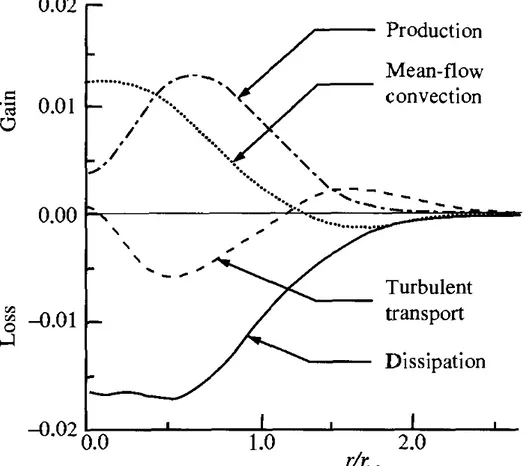
For the self-similar round jet the turbulent kinetic energy budget is shown in Figure 1. The quantities plotted are the four terms in equation (1.2.14) normalized by U0
3
/r1 / 2 . The
contributions are production, P; dissipation, ε; mean flow convection, −D k / D t ; turbulent trasport −∇⋅T ' . While production and mean flow convection are historically measured with uncertainties within 20%, the error on dissipation and turbulent transport can be as big a a factor of two or more.
Along the jet, dissipation is a dominant term. Production peaks at r /r1 /2≈0.6 , where the ratio P /ε≈0.8 . At the edge of the jet production goes to zero, and dissipation is balanced by the transport.
Figure 1: The turbulent kinetic energy budget in the self-similar round jet. Quantities are normalized by U0 and r1/2. (Panchapachesan & Lumely 1993)
1.3 Wall bounded flows
The vast majority of turbulent flows are bounded by one or more surfaces. Examples of internal flows are channel and pipe flows, while external flows are encountered when dealing with boundary layers. In this thesis it will be presented a simulation of a channel flow, so it's appropriate to give some background theory of his fundamental flow. Central issues are the mean velocity profiles, the friction laws and the turbulent energy balance, that will now be discussed.
Channel flow
Consider the flow along a rectangular duct
(
Lδ≫1
)
of large aspect ratio(
bδ≫1
)
. The resulting mean flow is predominantly in the longitudinal (or x) direction, while the mean velocity varies mostly in the transversal (or y) direction. All the flow statistics are independent of the spanwise (or z) position.Focusing the study on the fully developed region (so large values of x) the flow results statistically stationary and one-dimensional (varies only along y).
For the channel flow we define two velocities, and their respective Reynolds numbers:
•centreline velocity U0≡〈U 〉y=δ , ℜe0≡
δU0 ν •bulk velocity ̄U ≡1 δ
∫
0 δ 〈U 〉dy , ℜe≡(2 δ) ̄U ν .Balance of mean forces
Since 〈W 〉=0 and d 〈U 〉
dx =0 , from the continuity equation involving the mean velocities components we can say that:
d 〈V 〉
dy =0 (1.3.1)
and considering the impermeability condition at the wall we conclude that 〈V 〉=0 for all y. The mean momentum balance in y direction is then:
0=− d dy〈v 2 〉−1 ρ ∂〈p 〉 ∂y (1.3.2)
〈v2〉+〈p〉/ρ= p
w(x )/ρ ,where pw=〈p (x ,0,0)〉 . (1.3.3) This is useful to deduce that the mean axial pressure gradient is uniform across the flow:
∂〈p 〉 ∂x =
d pw
d x . (1.3.4)
The mean momentum balance in x direction is:
0=νd 2〈U 〉 dy2 − d dy〈u v 〉− 1 ρ ∂〈p 〉 ∂x (1.3.5)
and can be rewritten as:
dτ dy=
d pw
dx (1.3.6)
where the total shear stress is defined as:
τ( y)≡ρ νd 〈U 〉
dy −ρ〈u v 〉 (1.3.7)
Since τ is a function of only y, and pw is a function of only x, it's clear from (1.3.6) that both d τ /dy and d pw/dx are constant. Taking the boundary conditions into consideration:
τ(y)=τw
(
1− yδ
)
, where τw≡τ (0) . (1.3.8)The normalization of the wall shear stress is referred to as skin friction coefficient, based on the centreline or on the bulk velocity:
cf≡ τw 1 2ρU0 2 , CF≡ τw 1 2ρ ̄U 2 . (1.3.9)
The flow is driven by the drop in pressure between entrance and exit. In the fully developed
flow region there is a constant negative mean pressure gradient ∂〈p 〉 ∂x =
d pw
dx balanced by the
shear stress gradient d τ dy =−
τw δ .
Near wall shear stress
The total shear stress is the sum of viscous stress and Reynolds stress. At the wall the no slip condition U (x ,t )=0 makes it so that the Reynolds stress is zero. So at the wall the shear stress is entirely of viscous origin:
τw=ρ ν
(
d 〈U 〉dy
)
y=0. (1.3.10)
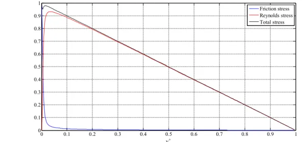
Profiles of the viscous and Reynolds shear stresses obtained with a DNS are shown in Figure 2. It's clear that close to the wall the viscosity ν and the wall shear stress τw are important parameters. From these quantities (and ρ) we define some viscous scales to be used near the wall:
•friction velocity uτ≡
√
τw ρ •viscous lengthscale δν≡ν√
ρ τw= ν uτ•friction Reynolds number ℜeτ≡
uτδ ν = δ δν •wall units y+ ≡ y δν =uτy ν
Different regions in the near wall flow are defined based on y+ . The viscous wall region
Figure 2: Profiles of the viscous shear stress, and the Reynolds shear stress in turbulent channel flow. DNS data from Jimenez (2008), Re=2000.
0 0.1 0.2 0.3 0.4 0.5 0.6 0.7 0.8 0.9 1 0 0.1 0.2 0.3 0.4 0.5 0.6 0.7 0.8 0.9 1 y+ Friction stress Reynolds stress Total stress
(y+
<50) is directly affected by molecular viscosity, while the outer region ( y+
>50) can neglect viscous effects. Within the viscous region there's the viscous sub-layer ( y+
<5) where the Reynolds shear stress is negligible compared to the viscous stress.
Mean velocity profiles
Channel flow is completely specified by ρ, ν, δ, uτ. With no assumptions and adopting a non
dimensional function Φ (to be determined) we can write: d 〈U 〉 dy = uτ y Φ
(
y δν ,y δ)
(1.3.11)keeping in mind that δν is the appropriate lengthscale in the near wall region, while δ is
suitable for the outer region.
The law of the wall
Following Prandtl hypothesis, close to the wall the mean velocity profile is determined by the viscous scales. Mathematically Φ asymptotically tends to a function of only y /δν as y /δ → 0 :
d 〈U 〉 dy = uτ y Φ1
(
y δν)
, for y δ≪1 (1.3.12) where Φ1(
y δν)
=y /δ → 0lim Φ(
y δν, y δ)
. (1.3.13) Defining u+ (y+ ) as u+ ≡〈U 〉 uτ (1.3.14) we can rewrite the previous relation as:du+ dy+= 1 y+Φ1(y + ) (1.3.15)
which after integration is the law of the wall:
u+ =fw(y+ )=
∫
0 y+ 1 y ' Φ1(y ' )dy ' . (1.3.16)Note that, for y
δ≪1 , u
from transition there is experimental proof that the function f w(y
+
) is universal for channel, pipe and boundary layers. The form of the function f w(y
+)
can be determined for small and large values of y+ .
Viscous sub-layer
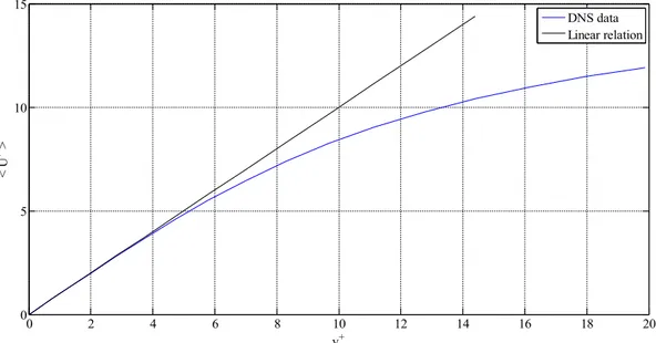
At the wall the no slip condition imposes fw(0)=0 , fw' (0)=1 . Using a Taylor expansion:
fw(y+)=y++Ο(y+2) (1.3.17)
As shown in Figure 3 the linear relation holds well for the viscous sub-layer ( y+
<5) .
The log law
For larger y+ we suppose that viscosity has little effect, so that Φ
1 assumes a constant value: Φ1(y + )=1 k for y δ≪1 , y +≫1 (1.3.18)
where k is the Von Kármán constant. So in this region the mean velocity gradient is given by:
du+
dy+=
1
k y+ (1.3.19)
which easily integrates to give the log law:
Figure 3: Near wall profiles of mean velocity from the DNS of Jimenez (2008), Re=2000.
0 2 4 6 8 10 12 14 16 18 20 0 5 10 15 y+ < U + > DNS data Linear relation
u+
=1
k ln ( y +
)+B . (1.3.20)
The values of the constants are determined experimentally and are taken to be within 5% of
k =0.41 , B=5.2 . (1.3.21)
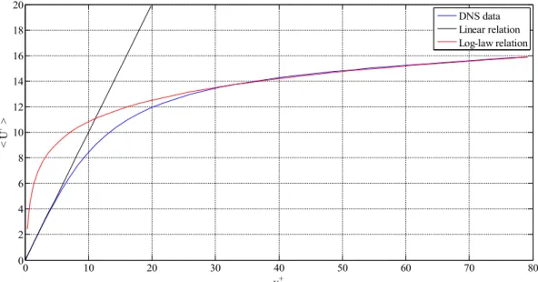
As shown in Figure 4 the law holds very well for y+
>30 and y
δ<0.3 . The region between the viscous sub-layer and the log-law region is called buffer layer, where transition form viscosity dominated to turbulence dominated flow occurs.
The velocity defect law
In the outer layer ( y+>50) we assume that Φ becomes independent of the viscosity
Φ0
(
y δ)
=y/δlimν→∞ Φ(
y δν ,y δ)
(1.3.22) leading to: d 〈U 〉 dy =Φ0(
y δ)
. (1.3.23)Integrating from a generic y/δ to the centre of the channel we obtain the velocity defect law:
U0−〈U 〉 uτ =FD
(
y δ)
=∫
y /δ 1 1 y 'Φ0(y ' )dy ' . (1.3.24)The velocity defect is the difference between the centreline velocity and the mean velocity. Figure 4: Near wall profiles of mean velocity, DNS data from Jimenez (2008), Re=2000.
0 10 20 30 40 50 60 70 80 0 2 4 6 8 10 12 14 16 18 20 y+ < U + > DNS data Linear relation Log-law relation
The law states that this difference, normalized by the friction velocity, depends on y/δ only. There is no suggestion that FD is universal, because it generally varies in different flows.
At high enough Reynolds number (generally Re > 104) there is an overlap region between the
inner layer ( y /δ<0.1) and the outer layer ( y /δν>50) . In this region both equations (1.3.18)
and (1.3.22) must be true, implying that y uτ d 〈U 〉 dy =Φ1
(
y δν)
=Φ0(
y δ)
, for δν≪y ≪δ . (1.3.25)This equation is satisfied in the overlap region only by Φ1 and Φ0 assuming a constant
value: y uτ d 〈U 〉 dy = 1 k , for δν≪y ≪δ . (1.3.26)
We can now determine the form of the velocity defect law for small y/δ to be: U0−〈U 〉 uτ =FD
(
y δ)
=− 1 k ln(
y δ)
+B1 , for y δ≪1 (1.3.27)where B1 is a flow dependent constant. To determine it's value, note that as shown in Figure 4 the log law is reasonably close to the DNS value even in the central part of the channel (0.3< y /δ<1) where no arguments support it. Extrapolating the centreline velocity from the log law we obtain a way to determine B1 :
U0−U0,log uτ
=B1 (1.3.28)
which results in a very small value since U0−U0,log is within 1% of U0 . DNS data lead to B1≈0.2 , while experimental results indicate B1≈0.7 .
Wall regions recap
Region Location Property
Inner layer y /δ<0.1
〈U 〉 determined by uτ and
y+ , independent of U 0
and δ
Viscous wall region y+<50 Significant contribution to the
shear stress due to viscosity
Viscous sub-layer y+
<5 Reynolds shear stress is
negligible compared to viscous
Outer layer y+>50 Negligible effect of viscosity
on 〈U 〉
Overlap region y+>50, y /δ<0.1 Present only at high Reynolds
Log law region y+
>30, y /δ<0.3 Log law holds
Buffer layer 5< y+
<30
Transitional region between viscous and turbulent dominated flow
The friction law
The aim is now to determine the Reynolds number dependence of the skin friction coefficient an other relevant quantities.
A good estimate of the bulk velocity come from the application of the log law to the whole channel. As stated before there are small deviations near the centreline, while the substantial deviations in the near wall region can be overlooked since they have a negligible contribution to the integral.
With this approximation:
U0− ̄U uτ =1 δ
∫
0 δ U 0−〈U 〉 uτ dy≃1 δ∫
0 δ −1 kln(
y δ)
dy= 1 k≈2.4 (1.3.29)Consider the log law in the inner layer 〈U 〉 uτ =1 kln
(
y δν)
+B (1.3.30)and in the outer layer
U0−〈U 〉 uτ =−1 k ln
(
y δ)
+B1 (1.3.31)combining them leads to:
U0 uτ =1 k ln
(
δ δν)
+B+ B1=1kln[
ℜe0(
U0 uτ)
−1]
+B+B1 (1.3.32)which is independent of y. Solving this for Uo/uτ we can calculate (for each given ℜe0 ) the
skin friction coefficient, using:
cf≡ τw 1 2ρU0 2=2
(
uτ U0)
2 (1.3.33)and with approximation (1.3.29) also
CF≡ τw 1 2ρ ̄U
2 . (1.3.34)
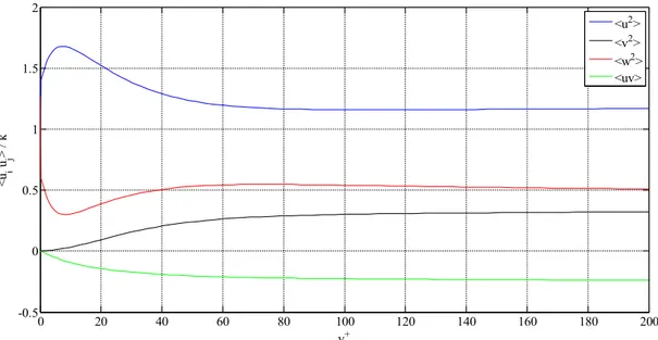
Reynolds stresses
Consider the DNS data at Re = 13'750 shown in Figure 5, Figure 6 and Figure 7. The flow is divided into three regions:
•viscous wall region for y+
<50
•log law region for y+>50, y /δ<0.3 or equivalently 50< y+<120
•core region for y /δ>0.3 or equivalently y+
>120
In the log law region there is approximate self-similarity. The normalized Reynolds stresses 〈uiuj〉
k are almost uniform, as is the production to dissipation ratio P
ε and the normalized
mean shear rate S k
ε . Moreover, production and dissipation are in balance, meaning P ε≈1 . In the core region the mean velocity gradient and the shear stress vanish, leading to P → 0.
In the viscous wall region, production, dissipation, turbulent kinetic energy and anisotropy achieve their peaks. Consider the fluctuation velocity components near the wall (small y) at a fixed point in space and time, expressed through a Taylor expansion:
u=a1+b1y+c1y2+…
v=a2+b2y+c2y2+…
w=a3+b3y+c3y2
+…
(1.3.35)
for the no slip condition and the impermeability at the wall a1=a2=a3=0 . Since u and w are zero at the wall for every x and z, we can state that
(
∂u ∂x)
y=0=0 and
(
∂w ∂z)
y=0=0 (1.3.36)
so for the continuity equation:
(
∂v ∂y)
y=0=0=b2 . (1.3.37)
This means that close to the wall the flow has only two components, i.e. the motion occurs in planes parallel to the wall.
Taking the mean of the series products gives the Reynolds stresses:
〈u2〉=〈b 1 2〉y2+… 〈v2 〉=〈c22〉y4+… 〈w2 〉=〈b32〉y2+… 〈u v 〉=〈b1c2〉y3+… (1.3.38)
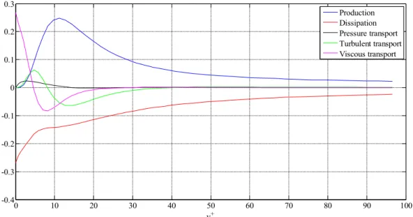
For fully developed channel flow, the turbulent kinetic energy balance equation is:
P−̃ε+νd 2k dy2− d dy〈 1 2ν ̄u⋅̄u 〉− 1 ρ d dy 〈 νp' 〉=0 (1.3.39)
where the terms are respectively production, pseudo-dissipation, viscous diffusion, turbulent convection and pressure transport.
Peak production occurs in the buffer layer at y+≈12 . Here P
ε≈1.8 so the excess energy is transported away. Pressure transport is very small. Turbulent convection transports both in the log wall region and in the near wall region. Viscous diffusion transports energy all the way towards the wall. The dissipation at the wall is balanced by the viscous transport,
ε=̃ε=νd
2k
dy2 , for y =2. (1.3.40)
Figure 5: Reynolds stresses and kinetic energy normalized by the friction velocity against y+ from DNS of channel flow
at Re=2000 (Jimenez 2008). 0 20 40 60 80 100 120 140 160 180 200 -1 0 1 2 3 4 5 6 7 8 9 <u2> <v2> <w2> <uv> kinetic energy
Figure 6: Profiles of Reynolds stresses normalized by the turbulent kinetic energy from DNS of channel flow at Re=2000 (Jimenez 2008). 0 20 40 60 80 100 120 140 160 180 200 -0.5 0 0.5 1 1.5 2 y+ <ui uj > / k <u2> <v2> <w2> <uv>
Figure 7: Profiles of the energy balance components from DNS of channel flow at Re=2000 (Jimenez 2008). 0 10 20 30 40 50 60 70 80 90 100 -0.4 -0.3 -0.2 -0.1 0 0.1 0.2 0.3 y+ Production Dissipation Pressure transport Turbulent transport Viscous transport
1.4 Free shear flows
The most commonly free shear flows are jets, wakes and mixing layers. The main characteristic of these flows is that they are away from walls so that the turbulence in the flow is caused only by differences in the mean velocity. Most of the experimental and numerical work in this thesis is about round jets, so the well known theory for this flow is now reminded here.
Round Jet flow
A round jet consist ideally of a Newtonian fluid, flowing steadily through a round nozzle of diameter d, which produces a flat top-hat velocity profile UJ. The jet flow enters an ambient filled
with the same fluid, which is at rest at infinity. The flow is also statistically stationary and axisymmetric, hence all statistics are independent of the time and the azimuthal coordinate ϑ. The velocity components along the cylindrical coordinate system (x , r , θ) are respectively
(U , Ur, Uθ) .
The flow is completely defined by Uj, d and v so the only non-dimensional parameter defining
it is ℜe=UJd /ν , even if in practice there is some dependence on details of the nozzle and the surroundings (Schneider 1985; Hussein 1994).
The mean velocity field
As expected the mean velocity is predominantly in the axial direction, with the mean azimuthal velocity being zero and the mean radial velocity being one order of magnitude smaller.
Defining the centreline velocity as
U0(x )≡〈U ( x ,0 ,0)〉 , (1.4.1)
and the jet's half width, r1/ 2 , as
〈U ( x , r1/ 2(x ), 0)〉=
1
2U0(x ) , (1.4.2)
one can observe that after an initial development region (say 0≤x /d ≤25 ) the axial mean velocity profile becomes self-similar. This means that as the jet decays and spreads, the mean velocity profile changes, but with proper scaling the shape of the profile is preserved.
To further investigate the jet self-similarity, it is necessary to determine the variation of
U0(x ) and r1/ 2(x ) . In Figure 9 the data for (the inverse of) U0(x ) is plotted against x/d,
resulting in a linear behaviour. The intercept of this line with the abscissa defines the so called “virtual origin”, denoted by x0 . The mathematical relation describing this trend is
U0(x) Uj
= B
(x−x0)/d
, (1.4.3)
where B is an empirical constant called velocity decay. Note that equation (1.4.3) does not formally hold in the development region, and is artificially prolonged there with the only purpose of calculating the virtual origin.
The empirical law for the jet's half width is
r1/ 2(x )=S (x− x0) , (1.4.4)
where S is the (constant) spreading rate. The law again holds only in the fully developed region. Since U0(x )≈ x−1 and r1/ 2(x )≈x the local Reynolds number ℜe0(x )=U0(x )r1 /2(x)/ν
is independent of x. The constants B and S where object of several experiments, summarized in the following table:
Panchapakesan &
Lumley (1993) Hussein (1994) hot-wire data Hussein (1994) laser doppler data
Re 11'000 95'500 95'500
S 0,096 0,102 0,094
B 6,06 5,90 5,80
From the table it appears that the spreading rate and the decay velocity are independent of Re for a turbulent and fully developed jet, the only differences being due to experimental uncertainties.
However, even if the flow shows no dependence of Re in the mean axial velocity profile and in the spreading rate after proper scaling, the Reynolds number still influences the absolute size of the small scale structures, making them smaller for larger Reynolds.
The cross stream similarity variable can be taken to be either
ξ≡r /r1 /2 , (1.4.5)
or
η≡r /(x− x0) , (1.4.6)
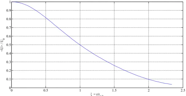
the two being related by η=S ξ . The self-similar mean velocity profile is defined as
f (η)= f (ξ)=〈U ( x , r ,0)〉/U0(x) , (1.4.7) and shown in Figure 9 for the axial component.
Figure 8: The variation with axial distance of the mean velocity along the centreline in a turbulent round jet, Re=95500. Symbols, experimental data from Hussein (1994); line, equation (1.4.3).
0 10 20 30 40 50 60 70 80 90 100 0 2 4 6 8 10 12 14 16 18 x/d Uj / U0 ( x)
Figure 9: Self-similar profile for the mean axial velocity in the self-similar round jet. (Hussein 1994)
0 0.5 1 1.5 2 2.5 0 0.1 0.2 0.3 0.4 0.5 0.6 0.7 0.8 0.9 1 ξ = r/r1/2 <U > / U 0
The mean radial component can be calculated from the continuity equation, resulting smaller by a factor of 40 compared with the axial component. The radial velocity becomes negative at the jet far ends, meaning that flow is actually being entrained form the ambient into the jet.
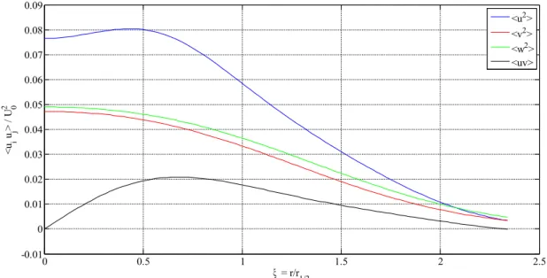
Reynolds stresses
The fluctuating velocity components in the cylindrical coordinate system are (ux, ur, uθ) so
it follows that in the turbulent round jet the Reynolds-stress tensor is
⟦
〈ux2〉 〈uxur〉 0 〈uxur〉 〈ur2〉 0 0 0 〈uθ 2 〉⟧
, (1.4.8)because 〈uxuθ〉 and 〈uruθ〉 are zero for axial symmetry.
The Reynolds stresses are also self-similar, i.e. the profiles of 〈uiuj〉/U0(x) 2
plotted against the radial coordinates ξ=r /r1 /2 or η=r /(x− x0) collapse for all x beyond the
development region as in Figure 10.
The local turbulence intensity is defined as u ' /〈U 〉 where u' is the root mean square (rms) velocity fluctuation u ' ≡
√
(〈u2〉) . At the edge of the jet, although the Reynolds stress decays, the ratio increases without bounds, as in Figure 11, starting from a centreline value of 0,25.
Figure 10: Profiles of Reynolds stresses in the self-similar round jet. (Hussein 1994)
0 0.5 1 1.5 2 2.5 -0.01 0 0.01 0.02 0.03 0.04 0.05 0.06 0.07 0.08 0.09 ξ = r/r1/2 <ui uj > / U 0 2 <u2> <v2> <w2> <uv>
Figure 11: The profile of local turbulence intensity in the self similar round jet. Blue line, data from Hussein 1994; green symbols, data from our facility.
0 0.5 1 1.5 2 2.5 0.2 0.4 0.6 0.8 1 1.2 1.4 1.6 ξ = r/r1/2 u rm s / <U > Hussein 1994 Exp data
1.5 Hot wire anemometry
Nowadays there are several techniques to estimate the velocity field in an experimental set-up. The main candidates are usually hot-wire anemometry (HWA), laser Doppler velocimetry (LDV) and particle image velocimetry (PIV). For the present experiments we choose HWA, mainly because of it's excellent temporal resolution. Spatial resolution is however a different problem, which is analysed in section (1.6), that can greatly affect the accuracy of measurements.
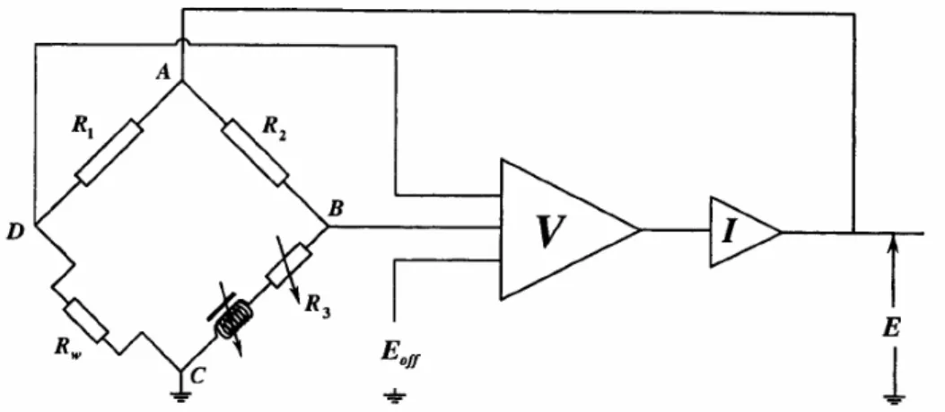
In HWA, a small wire heated by an electric current is placed in the flow. An electronic circuit connected to the wire measures the heat transferred to the flow that invests the wire, which is proportional to the flow velocity. We operate the wire in Constant Temperature Anemometry (CTA) mode, since the wire is maintained at a constant temperature with a feedback circuit as in Figure 12. The hot wire, shown between C and D, it is part of a Wheatstone bridge, such that the wire resistance is kept constant over the bandwidth of the feedback loop. Since the hot wire voltage is a simple potential division of the output voltage, the output voltage is normally measured for convenience.
Since the circuit response is heavily dependent upon the individual hot wire, the feedback circuit must be tuned for each hot wire (Dantec 1986). Although strictly it is necessary to test the hot wire with velocity perturbations to optimise the frequency response, a much simpler electronic test has been developed that injects a small voltage square wave into the Wheatstone bridge. It has been shown (Freymuth 1977), that the optimum circuit performance is found when the output response is approximately that shown in Figure 13. The square wave test allows a quick estimation of the frequency response, although it has been shown (Moss 1992) that any contamination of the wire reduces the frequency response without any apparent effect on the pulse response.
General hot-wire equation
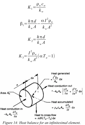
To examine the behaviour of the hot wire, the general hot wire equation must first be derived. This equation will be used to examine both the steady state response of the hot wire, discussed here, and its frequency response, discussed later. By considering a small circular element of the hot wire, as in Figure 14, a power balance can be performed, assuming a uniform temperature over its cross-section: I2Rwδx=ρwcw∂Tw ∂t A δ x+kwA ∂Tw ∂x +h π d (Tw−Ta)δx−kwA
(
∂Tw ∂x + ∂2Tw ∂x2 δx)
+σ ε(Tw 4 −Ta 4 ) πd δ x (1.5.1)where on the left hand side there is the power produced by Joule effect. In the right hand side we find the power accumulated in the wire, the incoming power due to conduction, the power loss to convection, the outgoing power due to conduction and the irradiated power respectively.
The quantities in equation (1.5.1) are: I current intensity in the wire, Rw wire resistance, ρw wire density, cw wire specific heat, Tw heated wire temperature, kw wire thermal conductivity, h convective heat transfer coefficient, Ta fluid ambient temperature, σ Stephan-Boltzmann constant and ε emissivity of the wire.
This can be simplified neglecting radiation (Højstrup 1976), to give the general hot-wire equation: K1 ∂Tw ∂t = ∂2Tw ∂x2 −β1Tw+K2Ta−K3 . (1.5.2)
Figure 13: Optimum square-wave test response. (Bruun 1995)
The constants are given by: K1= ρwcw kw (1.5.3) β1=h π d kwA− αI2 ρw kwA2 (1.5.4) K2=h π d kwA (1.5.5) K3=I 2 ρw kwA2( αTa−1) (1.5.6)
The two main assumptions made in deriving equation (1.5.2) are that the radial variations in wire temperature and the radiation heat transfer are negligible: both of these will be justified briefly. The radiation term in equation (1.5.1) can be compared with any other term to assess its relative importance: the term chosen here is the convective heat loss term in equation (1.5.1), giving a ratio:
Ratio= σ ε h Ta(Tw
4
−Ta4) . (1.5.7)
Typical flow conditions over a typical hot wire give a ratio of 0.048 %.
The effects of radial variations are slightly more complex, but a simple case can be developed whereby the temperature is assumed to vary only in the radial direction. Performing a heat balance on the wire gives:
−I2ρ w kwA2 = 1 r ∂ ∂r
(
∂T ∂r)
(1.5.8)If the change in resistivity with temperature is neglected, this yields the solution: Figure 14: Heat balance for an infinitesimal element.
Tw(r)=const− I 2ρ w kwA2 r2 4 , (1.5.9)
where the constant is found from an energy balance at the surface. The maximum change across the wire as a ratio of the difference in temperature driving the heat transfer is then:
Ratio=1 4
k
kw Nu , (1.5.10)
where Nu is the Nusselt number, defined as Nu=h dw/kw , which is a non-dimensional parameter for the ratio between convectional and conductive heat exchange.
For typical conditions at stage exit, the ratio is 0.022 %. Since these two effects are clearly negligible, equation (1.5.2) can be used as the general hot wire equation.
Steady state solution
The general steady state solution to equation (1.5.2), assuming that ̄β1>0 , is found by applying the boundary condition and defining the mean wire temperature, denoted with an upper bar, along the axial coordinate of the wire x (see also Figure 14):
̄ Tw= ̄Ta at x=±1 , (1.5.11) Tm= 1 2 l
∫
−l +l ̄ Twdx . (1.5.12)The non-dimensional steady state wire temperature distribution is then:
̄ Tw− ̄Ta Tm− ̄Ta =
[
1−cosh (√
̄β1x ) cosh (√
β̄1l)]
[
1− 1 (√
̄β1l)tanh(√
̄β1l)]
, (1.5.13)which is only a function of the Biot number
√
β̄1l as seen in Figure 15.A heat balance can then be performed over the whole wire, assuming that the flow conditions are uniform over the wire:
̄I2R
w= ̄Hcond+ ̄Hconv . (1.5.14)
The two heat transfer components can be found from the flow conditions and the wire temperature distribution:
̄
̄
Hcond=2 kwA
∣
∂ ̄Tw∂x
∣
x=l, (1.5.16)
to give a steady state heat transfer equation:
̄I2R
w=2 π ̄hcd l (Tm−̄Ta) , (1.5.17)
where the corrected heat transfer coefficient is given by:
̄ hc=̄h+ d kw 4 l
(
√
̄β1tanh(√
β̄1l) 1−tanh(√
̄β1l)√
̄β1l)
. (1.5.18)If the Biot number is larger than approximately 3, as is usually the case, in terms of Nusselt number this approximates to (Bradshaw 1971):
Nuc=Nu+ d 2 l
√
kw
k
√
Nu (1.5.19)giving the steady state calibration equation:
̄ Ew2
=2 π k l RwNuc(Tm−̄Ta) , (1.5.20)
where the temperature dependent wire resistance is set by adjusting the current flow in the Wheatstone bridge. To reduce the proportion of heat transfer by conduction for given flow conditions the wire length to diameter ratio must thus be increased. Although the conduction end effect can be compensated out using equation (1.5.19), this is normally done automatically in the calibration. Equation (1.5.20) shows that the variations in the wire voltage are only dependent upon fluctuations in the Nusselt number and the temperature difference between the hot wire and the flow: both of these will now be examined.
Figure 15: Steady state temperature distribution. (Freymuth 1979)
Nusselt number dependence
Due to the general engineering importance of heat transfer from a heated cylinder, the dependence of the Nusselt number on the flow conditions has been the subject of much research. The Nusselt number, as stated before, is a non-dimensional heat transfer coefficient, Nu=h d /k which is the ratio of of the convective to the conductive heat transfer. The most general relationship states the dependence of Nu from several parameters (Bruun 1995):
Nu=Nu(ℜ e , Pr , Kn , M , l /d , ΔT /Ta) , (1.5.21)
where the Reynolds number ℜe=Ud /ν , Mach number M =U /a and Prandtl number Pr=ν/α are defined using the kinematic viscosity of the fluid ν , the velocity of sound a, and the thermal diffusivity α . The Knudsen number Kn=λ/ d represents the ratio between the gas mean free path λ and the wire diameter. The influence of the wire length/diameter ratio is due to the conduction end effects. In principle it would be possible for a given hot-wire probe to find an expression for the Nusselt number in terms of the non-dimensional quantities in equation (1.5.21).
In practice, however, (keeping in mind that hot-wire probes are miniature devices) such a general relation would give large errors for small deviations. It is however possible to further simplify the above relation with some assumptions:
•incompressible flow (eliminates the Mach number dependence) •standard density flow (eliminates the Knudsen number dependence) •infinitely long wire (eliminates both l/d and ΔT /Ta dependence).
This idealised problem was solved by King (1914), resulting in King's law:
Nu=Nu(ℜ e , Pr)=1+
√
2 π(Pr ℜe )1
2 . (1.5.22)
For HWA applications this translates into:
E2=A+B U
eff n
(1.5.23) where A, B and n are variables dependent on several quantities listed in relation (1.5.21), and the effective cooling velocity Ueff is given by Jorgensen's equation:
Ueff2 =Un2 +kt2U t 2 +ks2U s 2 , (1.5.24)
where in the reference system of a single wire Un, Ut,Us are respectively the normal, tangential and bi-normal velocity components; kt, ks are the yaw and pitch factors equal to ≈0.2 and
For a given probe operated in a low Mach number flow the fluid properties are fairly constant and if additionally the temperature difference between the wire and the flow temperature is kept constant (this is known as constant temperature anemometry (CTA)) the variables A, B and n in equation (1.5.23) will loose their dependency on the mentioned dimensionless quantities.
Figure 16 shows a typically observed Nu≈ ℜe0,5 (equivalent to E2≈U
eff
0,5 ) functionality,
which shows a fairly good constancy of the variables in equation (1.5.23) over a quite large Reynolds number range. The constants A, B and n are usually determined by means of a calibration against a known flow field.
Temperature dependence
The measured wire voltage is also dependent upon the temperature difference between the wire and the flow (1.5.21). Unless this temperature difference is measured or already known a measurement error will result, although this error can be minimised for small temperature fluctuations by operating the wire at a high temperature and calibrating the wire at the mean flow temperature. A means of compensation will otherwise be required: there are two main practical ways (Bruun 1995):
1. Automatic compensation: Use a temperature sensor in the Wheatstone bridge.
2. Analytical correction: Measure the flow temperature separately and compensate using the heat transfer equation.
Since automatic compensation has a bandwidth of approximately 100 Hz, analytical correction is the only means of compensation at most experimental frequencies, provided the possibility of having time-resolved temperature measurements.
Figure 16: Nu as a function of Re for hot wire in air. (Alfredsson 2005)
Technique limitations
The features of hot-wire anemometry were already mentioned, namely its continuous signal and its ability to detect very fast fluctuations. If several hot-wires are placed close to each other or on the same probe two or three velocity components as well as velocity gradients can be measured instantaneously and simultaneously. But there are limitations to what can be measured. Most of the limitations can directly be derived from the assumptions made within this chapter. These assumptions begin to fail in very low velocity regions (where natural convection becomes important), separation regions (i.e. backflow, since hot-wires cannot distinguish between upward or downward cooling) or in very close vicinity of solid surfaces (since the heat sink represented by the surface is not taken into account by the calibration) .
1.6 Resolution effects in hot wire measurements
Accurate measurement of the statistics in a turbulent flow is important to further advance the fundamental knowledge in the field. To this day the study of resolution effects was mainly focused on turbulent boundary layers, where the small scale structures are small enough to appreciate the issue. Hot-wire anemometry (HWA) is the most popular experimental technique for turbulent boundary layer research, given its unsurpassed temporal and spatial resolution. A growing number of discrepancies reported in the literature by different groups of researchers led to the investigation on how the lack of resolution can affect measurements. The staple work in this field is the experimental investigation on spatial resolution by Ligrami & Bradshaw (1987), referred to from now on as LB87.
Even if in the present work turbulent boundary layers are not directly considered, similar effects to the ones reported in this chapter can potentially occur in other turbulent flows, such as the jet or the channel. It was deemed appropriate to report the latest results in resolution effects, but the actual impact on jet and channel flow measurements should be far less, because the turbulent structures are bigger than in the boundary layer.
Methodology
The spatial attenuation (filtering) caused by an idealized spanwise sensor is a function of the integral of the velocity fluctuations across the element. In turbulent flows these fluctuations are time dependent, and composed of multiple overlapping and interacting scales. The degree of attenuation on the single spanwise element is highly dependent on the spectral composition of turbulent fluctuations. Specifically one must consider the width of the energetic fluctuations compared to the spanwise length of the sensor element. This requires spectral information in the spanwise direction, which are today available only from direct numerical simulations (DNS).
In recent literature two different approaches to the problem are found. One is to collect many experimental data from previous works, involving different probe lengths, l/d ratios and Reynolds number, and extrapolate the filtering effect caused by these factors. The other is to consider a DNS of the flow and, from these “exact” data, investigate the effects of resolution by filtering the data according to different probe length.
Both approaches seem to lead to the same conclusions (Hutchins 2009), but the debate is still open on some issues. As an example of the effects of spatial resolution effects, we report the near wall peak attenuation and the outer hump generation.