Tactile perception - Perception of tactile distance changes with body site: a neural network modelling study.

SECONDA FACOLTÀ DI INGEGNERIA CON SEDE A CESENA CORSO DI LAUREA MAGISTRALE IN INGEGNERIA BIOMEDICA

“TACTILE PERCEPTION – PERCEPTION OF

TACTILE DISTANCE CHANGES WITH BODY SITE:

A NEURAL NETWORK MODELLING STUDY.”

Tesi in

Sistemi Neurali LM

Relatore Presentata da Prof.ssa Elisa Magosso Enrico Altini

Correlatore

Dr. Matthew Longo

III SESSIONE

                                        To my family: Mum, Dad, Erika, Massimo,

and my sweet Gaia….                                                          

Ø

Computational  Model  

Ø

Synaptic  Connections  

Ø

Tactile  Perception  

Weber’s  Illusion

Introduction

Chapter 1

Tactile Information Processing and Tactile Distance Perception

Introduction………...5

1.1 Touch………..………6

1.2 Mechanoreceptors and Receptive Fields………...8

1.3 Somatic Sensory Cortex………...11

1.4 Cortical Neuron RF………...13

1.5 Tactile Illusion: Weber’s Illusion………..………...15

1.5.1 Homunculus………....17

1.5.2 Magnification Concept……….….……….……....19

1.5.3 Green Experiment……….….……….……...23

1.6 The Neural Network and the simplifying assumptions………...….……....19

Chapter 2

2.1.1 The two main layers..………..28

2.1.2 Application of 2 punctual stimuli: effects within the First Layer…...31

2.1.3 Application of 2 punctual stimuli: effects within the Second Layer...31

2.2 Mathematical description of the network……….35

2.2.1 First Layer of neurons (Area 1)..……….36

2.2.2 Second Layer of neurons (Area 2)…..……….40

2.3 Parameters and their values………..42

2.4 Activation of neurons step by step………...………43

II

Chapter 3

Simulations and results

Introduction……….……….62

The noise……….……….63

Threshold of activation……….………65

3.1 First Experiment………...66

3.1.1 Tactile Size Perception on the Hand vs Arm ………...66

3.1.2 PSE and IQR of the First Experiment……….…….71

3.1.3 Activation of neurons in the Hand and in the Arm ……….75

3.2 Second Experiment………...76

3.2.1 Student t-Test………...………76

3.3 Third Experiment………...82

3.3.1 Two Point Discrimination Threshold ………..………...82

3.3.2 Comparison with Green’s results……….……92

3.3.3 Rescaling Process results.………....93

3.4 Fourth Experiment………....97

3.4.1 Dependency on the stimuli dimension ………..………..97

3.4.2 Analysing of Area1’s output………...…105

3.4.3 Analysing of Area2’s output………...…105

3.4.4 Validation with t-Test………...………..106

3.4.4.1 First Layer: mean 3 vs Mean 4……….110

3.4.4.2 Second Layer: mean 3 vs Mean 4……….111

Chapter 4

4.2 The changed Parameters……….116

4.2.1 Parameters Alteration………...118

4.3 Alteration of the Parameters and Neural Network Behaviour …………...119

4.4 Average Difference between the two activation balls ………...………....139

4.5 Conclusion about the Sensitivity Analysis………...141

4.6 Sensitivity Analysis about the Activation Threshold………….…………142

III

Conclusions………...155

Bibliography ………....159

1

Distortions in the perception of the distance between two punctual stimuli applied on the skin surface of different body regions are called Weber’s Illusion. This illusion was confirmed by many experiments, in which subjects were asked to judge the distance between two stimuli applied on the skin surface of different body regions. Results have shown that the same distance between the stimuli was judged different for different body regions.

The concept that the distance on the skin is frequently misperceived is largely supported, but the neural mechanisms underlying this illusion are still far to be well understood. In particular, it is still unclear how the distance between two simultaneous tactile stimuli is codified at a neural level, and which brain areas are involved in this computation.

Weber’s Illusion may be partly explained considering the differences in receptors density of various body regions, and the distorted image about the body that our brain has inside the Primary Somatic Sensory Cortex (homunculus). However, these mechanisms seem not to be sufficient to explain the observed phenomenon: indeed, according to 100 years-experimental results, the biases in distance judgement are much smaller than imbalances that primary representation would suggest. In other words, the observed illusion is much smaller compared to the effect that the differences in receptor density, or cortical extent would produce. This has lead to the hypothesis that judging tactile distance may require the recruitment of additional brain areas, and mechanisms that operate to rescale – at least partially – information from primary representation, in order to preserve tactile size constancy throughout the body surface

That is, it has been proposed the occurrence of sort of “Rescaling Process” that operates to reduce this illusion toward a more verisimilar perception.

2

The occurrence of this rescaling process is supported by many neuroscience researchers; in particular, Dr. Matthew Longo from the Department of Psychological Sciences, Birkbeck University of London is conducting research on tactile distance perception and body representation, and its research supports this hypothesis. However, the neural mechanisms and circuits at the basis of this potential rescaling process are still largely unknown.

The aim of this thesis was to clarify the possible network organization, and neural mechanisms explaining the Weber’s Illusion and the rescaling process, by using a neural network model. Much of the work was conducted at the Department of Psychological Sciences, Birkbeck University of London, under the supervision of Dr. Matthew Longo.

In order to replicate Weber’s Illusion and rescaling process, the neural network has been organized in two main layers of neurons that may correspond to two functionally different cortical areas:

• First Layer of neurons (that performs the first processing of the external stimuli): this layer might mimic the Primary Somatic Sensory Cortex affected by cortical magnification.

• Second Layer of neurons (that further elaborates information from the previous layer): this layer may represent a Higher Cortical Areas (e.g. in temporo-parietal region) involved in the implementation of the Rescaling Process.

Neural networks have been constructed including synapses connection within each neuron layers (lateral synapses), and between the two neural layers (feed-forward synapses), and assuming that the activity of each neurons depends on its input via a static sigmoidal relationship, and a first order dynamics. In particular, by using the previous structure, I have implemented two different neural networks, for two different body regions (for example, the Hand and the Arm), characterized by different tactile resolution and cortical magnification to replicate the Weber’s Illusion and the Rescaling Process.

These models may help to understand the mechanism of the Weber’s Illusion, and to give a possible explanation of the Rescaling Process. Moreover, the

3

neural networks may help to understand how the brain can interpret the distance on the skin surface, and these models could be used to make new predictions to be verified later, in vivo, by tactile experiments on real subjects. It is important to underline that the developed models are mainly functional models and they are not intended replicate physiologic and anatomic details.

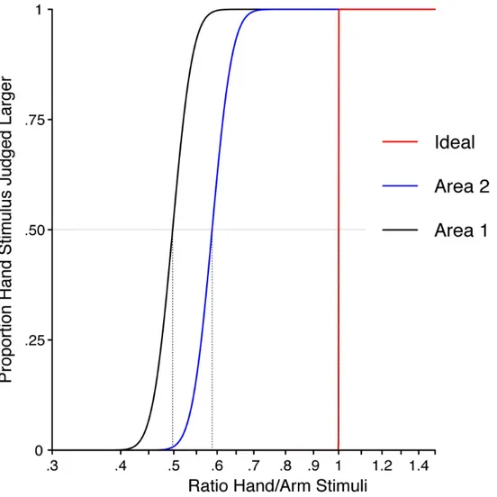
The main results achieved via the models are the reproduction of the Weber’s Illusion for the two different considered body regions (Hand and Arm), as reported in many articles about the tactile illusions. Weber’s Illusion was recorded from the output of the neural networks, and represented by graphics, trying to explain the reasons of these results.

The main part of this thesis was developed in the Department of Psychological Sciences, at Birkbeck, University of London under the supervision of Dr. Matthew Longo, for a period of 5 months. The contribute of Dr. Longo was very useful due to his great experience about experiments involved in the tactical perceptions. His help was directed especially toward the interpretation of the model outputs, giving suggestions about processing of network results, in order to obtain clearer information. Moreover, Dr. Longo has provided help in validation results, performing statistical test. Besides the benefit of interacting directly with an expert person as Dr. Longo, another benefit of may visit at the Birkbeck University was the improvement of my English, and the contact with a different university reality, as well as the experience of working in a team of researchers.

The present thesis is organized in four chapters.

The first chapter explains the theoretical aspects of the Weber’s Illusion, and the tactile processing information that starts from the skin surface of a body region, and continues through different layers in the cortex.

The second chapter is entitled “Mathematical Model”; it explains the network structure, provides a quantitative description of the model containing all mathematical formulas, explanation of each parameter, and provides example of neural activation within the two network layers.

4

Chapter 3 shows the results of the simulations: this chapter provide deep analyses of the output of the neural network in response to the application of an input (two punctual stimuli).

Finally Chapter 4 concerns the “Parameters Sensitivity Analysis”: in that Chapter, simulation results have been analysed after changing the value of one parameter at a time, in order to assess which parameters mainly affect network behaviour.

TACTILE INFORMATION

PROCESSING AND TACTILE DISTANCE

PERCEPTION

Introduction

The perception of distance for dual tactile pressures changes for different body regions. Over a century ago, Weber reported the concept that the distance on the skin is frequently misperceived. In the Weber’s illusion, the perception of distance between two tactile punctual stimuli is different in different parts of the body, increasing as the spatial acuity of the stimulated area increases.

Probably, the main reasons of this Illusion, are relative to the different size of the Receptive Field (RF) on the skin surface bonded to each cortical neuron, and the fact that the Primary Somatic Sensory Cortex reserves different amounts of area for representation of different body regions: for example, the Area involved in the perception of the hand, is much bigger than the Area about the back or the arm (homunculus).

Different extensions of cortical surface implicate different resolutions on different body regions: there are much more neurons in the brain involved to the hand, than the arm. Thus, the area inside the cortex reserved to the hand is bigger compare with the arm’s area. This means that the hand has a higher resolution in the comparison with the arm.

My thesis intends to implement a model able to simulate how the brain can interpret tactile stimuli on the skin surface in two different body regions. From the Weber’s experiment the application of two simultaneous stimuli (on the skin surface with a constant distance, on two different regions (like the hand and the arm) produce two different perceptions of distance.

DISTANCE PERCEPTION

6

As I stated above, the classical explanation of the Weber’s Illusion is the difference in the density of tactile receptors and cortical magnification across body parts. However, this explanation is unsatisfactory, because the illusion is much smaller than the differences in receptor density or cortical extent.

Therefore, there must be present a sort of rescaling process along the pathways of tactile information processing in the brain that might decrease this huge difference (relative to the homunculus dimension) and brings it to an acceptable proportion. It is clear that we feel a sort of distortion in the perceived distance, but basically it is kept down.

The neural mechanisms underlying this rescaling process are still largely unknown. Aim of this thesis is to contribute to clarify the neural mechanisms that may implement this rescaling, via a neural network modelling study. Of course, the model includes several simplifications and it doesn’t aspire to reproduce exactly the reality, also because the number of variables that should be considered is massive. This is mainly a conceptual model that, with the help of some hypotheses, tries to reproduce and interpret some experimental evidences (Weber’s illusion, distortions in perceive distance).

Before starting to explain my model, in this introduction I’m going to introduce few important concepts about the Receptive Field, the Primary Somatosensory Cortex, and the Homunculus.

1.1 Touch

Touch is mediated by mechanoreceptors in the skin and the tactile sensitivity is greatest on the hairless skin (glabrous), on the fingers, palm, sole of the foot and lips. When an object presses against the hand, the skin conforms to its contours. All mechanoreceptors sense these changes in skin contour, and they answer with a particular physiological function that will reach the Somatic Sensory Cortex inside the Central Nervous System.

DISTANCE PERCEPTION

7

All somatosensory information from the limbs and trunk is conveyed by dorsal root ganglion neurons. This kind of neuron is well suited to its two principal functions:

1. Stimulus transduction.

2. Transmission of encoded stimulus information to the central nervous system.

The cell body of these neurons lies in a ganglion on the dorsal root of spinal nerve. The axon has two branches, one direct to the periphery and the other one to the central nervous system.

Figure 1. 1 Position of the Dorsal Root Ganglion.

Mechanoreceptors and proprioceptors are innervated by dorsal root ganglion neurons with large diameter and myelinated axons that conduct action potential quickly. Thermal receptors and nocireceptors have smaller diameter axons that are thinly myelinated; these nerves conduct impulses very slowly. (“Principle of Neuron Science. Chapter 22: The Bodily Sense.” Kandel)

DISTANCE PERCEPTION

8

Neurologists distinguish between two classes of somatic sensation: epicritic and protopathic. Epicritic sensations involve aspects of touch and are mediated by encapsulated receptor. Instead, Protopathic sensation involves pain and temperature senses, and are mediated by receptors with bare nerve endings. In this thesis we will concentrate on Epicritic Sensations.

Information transmitted to the brain from mechanoreceptors in the hand, enabled us to feel the shape and texture of objects, type on computer keyboards, play musical instruments, etc. The ability to recognize objects placed in the hand on the basis of touch alone, is one of the most important and complex function of the somatosensory system. Tactile information about an object is fragmented by peripheral sensors, and must be integrated by the brain. In fact, an object stimulates a large number of receptors and sensory nerve fibres, each of which scans a little part of the object. Spatial properties are processed by populations of receptors that form many parallel pathways to the brain. It is the job of the central nervous system to reconstruct the correct shape of the object from the received fragmented information.

1.2 Mechanoreceptors and Receptive Fields

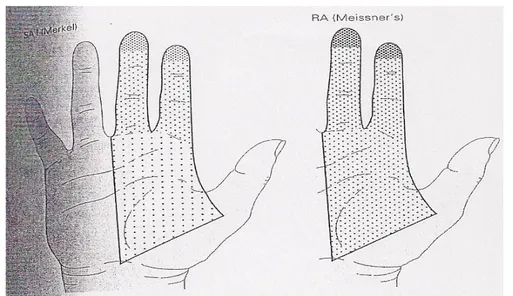
Mechanoreceptors differ in morphology and skin location. Histological and physiological studies have identified four major types of mechanoreceptors on the glabrous skin. Two of these are located in the superficial layers of the skin (Meissner’s corpuscle and Merkel disk receptor), and the other two in the subcutaneous tissue (Pacinian corpuscle and Ruffini ending). The small superficial receptors sense deformation of the papillary ridges in which they reside. The larger subcutaneous receptors sense deformation of a wider area of

DISTANCE PERCEPTION

9

skin that extends beyond the overlying ridges (“Principle of Neuron Science. Chapter 22: The Bodily Sense.” Kandel).

Figure 1. 2 Position of the Dorsal Root Ganglion.

Another important aspect is that mechanoreceptors on glabrus skin vary in the size and structure of their receptive field (RF).

The receptive field of a sensory neuron is a region of space on the skin in which the presence of a stimulus will alter the firing of that neuron. Receptive fields have been identified for neurons of the auditory system, the somatosensory system, and the visual system.In the somatosensory system, receptive fields are regions of the skin or of internal organs. Some types of mechanoreceptors have large receptive fields, while others have smaller ones.

DISTANCE PERCEPTION

10

Figure 1. 3 Example of Receptive Fields.

Large receptive fields allow the cell to detect changes over a wider area, but lead to a less precise perception. Thus, the fingertips are the most densely innervated regions of the skin in the human body, receiving approximately 300 mechanoreceptors nerve fibres per square centimetre, with small receptive field, which enable the ability to detect fine details. While the back and legs, for example, have fewer receptors with large receptive fields. Receptors with large receptive fields usually have a "hot spot", an area within the receptive field (usually in the centre, directly over the receptor) where stimulation produces the most intense response. It has to be considered that the density of receptors changes along the entire body. So, there are regions with a high density receptors (like hands), and regions with low density receptors (like trunk, or arms).

DISTANCE PERCEPTION

11

Figure 1. 4 The distribution of receptor types in the human hand varies.

Tactile-sense-related cortical neurons have receptive fields on the skin that can be modified by experience, or by injury to sensory nerves, resulting in changes in the field's size and position. In general these neurons have relatively large receptive fields (much larger than those of dorsal root ganglion cells). However, the neurons are able to discriminate fine details due to patterns of excitation and inhibition: I will explain this important concept in the next pages of this chapter.

1.3 Somatic Sensory Cortex

Sensory information is processed in a series of relay regions within the brain. There are three synaptic relay sites between sensory receptors in the skin, and the cerebral cortex. Mechanoreceptors in the skin send their axon to the caudal medulla, where they terminate in the gracile nuclei. These second order neurons project directly to the contralateral thalamus, terminating in the ventral posterior lateral nucleus. A parallel pathway from the principal trigeminal nucleus, which represents the face, ascends to the ventral posterior medial nucleus. The third order neurons in the thalamus send axons to the Primary Somatic Sensory Cortex, located in the post-central gyrus of the parietal lobe.

DISTANCE PERCEPTION

12

The Primary Somatic Sensory Cortex (S-I) contains four cytoarchitectural areas: Brodmann’s areas 3a, 3b, 1, and 2. Most thalamic fibres terminate in area 3a and 3b, and the cells in area 3a and 3b project their axons to areas 1 and 2. Thalamic neurons also send a small projection directly to area 1 and 2. Area 3b and 1 receive information from receptor in the skin, while area 3a and 2 receive proprioceptive information from receptors in muscles and joints. However all these areas are interconnected, so that, both serial and parallel processing are involved in higher-order elaboration of sensory information.

Figure 1. 5 Primary Somatic Sensory Cortex.

The Secondary Somatosensory Cortex (S-II), located on the superior bank of the lateral fissure, is innervated by neurons from each of the four areas of S-I. The fibres from S-I are required for the function of S-II. The S-II cortex projects to the insular cortex, which in turn innervates regions of the temporal lobe believed to be important for tactile memory.

Finally, other important somatosensory cortex areas are located in the posterior parietal cortex: Brodmann’s area 5 and 7. These areas receive input from both S-I and pulvinar (associational function). Area 5 integrates tactile information from mechanoreceptors in the skin with proprioceptive inputs from muscles and joint. This region also encapsulates information about the hands. Area 7 receives visual, as well as tactile, and proprioceptive inputs. The posterior parietal cortex projects to the motor areas, and plays an important role in sensory initiation and guidance of movement.

DISTANCE PERCEPTION

13

1.4 Cortical Neuron RF

The neurons in the primary somatic sensory cortex receive, at least, three synaptic connections beyond the peripheral receptors. Thus, their responses reflect information processed in the dorsal column nuclei, the thalamus, and in the cortex itself. They receive information from the skin, and they can be slowly, or rapidly adapting neurons.

Since each cortical neuron receive inputs form receptors in a specific area on the skin, cortical neurons also have receptive fields. All the cortical neurons are identify by their RF, as well as by their sensory modality. Any point on the skin is represented in the cortex by a population of cortical cells, connected to the afferents fibres that innervate that point on the skin. When a point on the skin is stimulated, the population of cortical neurons linked to the receptors at that location is excited. We perceive contact at a particular region on the skin, because a specific population of neurons in the brain is activated.

The receptive fields of cortical neurons are much larger than those of peripheral neurons. For example, the RF of a neuron in area 3b represents a composite of inputs from about 300-400 mechanoreceptors afferents. Receptive fields in higher cortical areas are even larger. A cortical neuron responds best to excitation in the middle of its receptive field; as the stimulation site is moved toward the periphery of the field, response becomes weaker until eventually no spikes is recorded.

A more complex receptive field structure emerges when the skin is touched in two or more points simultaneously. Stimulation of regions of skin surrounding the excitatory region of the receptive field of a cortical neuron, can reduce the excitatory response of the neuron, because afferent inputs surrounding the excitatory region are inhibitory. These regions of the receptive field are called the inhibitory surround. This spatial distribution of excitation, and inhibition is necessary to sharpen the peak of activity inside the brain. Inhibitory interneurons are present in the dorsum column nuclei, in the thalamus, and in the cortex itself. Inhibitory interneurons are fundamental to limit the spatial spread of excitation, in order to obtain a distinct recognition of simultaneous stimuli on the skin.

DISTANCE PERCEPTION

14

Figure 1. 6 Example of Surround Inhibition.

In this thesis project, we have implemented a neural network model that simulates the response to the application of two nearby tactile stimuli as input. Therefore is clear that the inhibitory process is a very important aspect to be considered. Especially, lateral inhibition can aid in two-point discrimination. We are able to perceive two points rather than one, because two distinct populations of neurons are activated in the cortex. If the stimuli are very close, the activity in the two populations tends to overlap, and the distinction between the two peaks might become blurred. However, the inhibition produced by each stimulus is summated in the overlap region. As a result of this more effective inhibition, the peaks of activity in the two corresponding populations become more sharpened, leading to a separation of the two populations.

DISTANCE PERCEPTION

15

Figure 1. 7 Stimulation of two adjacent points. Lateral Inhibitory networks suppress

excitation of the neurons between the points, sharpening the central focus, and preserving the spatial clarity of the original stimulus (solid line).

1.5 Tactile Illusion: Weber’s Illusion

In 1834 E. H. Weber described a tactile illusion. Two points kept equidistant moved over the body surface are felt to converge or diverge. The two points are perceived as converging, when passing from a high resolution region (hand) to a less sensitivity region (arm), and are perceived as diverging when passing from a low-resolution region to a highest one. This means that the same distance between the two stimulated points is perceived in different way on different body regions.

A possible explanation of this illusion may be found in the structure (size) of the RF along the whole body, and also in the variance of receptor density on the skin surface.

The size of the RFs, in a particular region of skin, establishes the capacity to determine whether one or more points are stimulated. If two points within the same receptive field are stimulated, the neuron will signal only one detection. But if the points are located in the receptive field of two different nerve fibres,

DISTANCE PERCEPTION

16

then information about both points of stimulation will be signalled. The contrast between active, and inactive fibre, seems to be fundamental for resolving spatial details, or to evaluate the distance between two points. Spatial resolution on various region of the skin can be quantified in humans by measuring their ability to perceive a pair of nearby stimuli as two different entities. The minimum distance between two detectable stimuli is called two point discrimination threshold.

Figure 1. 8 Two Point Discrimination Threshold along the body.

These variations are correlated with the RF dimension and with the innervation density of mechanoreceptors on the skin surface.

DISTANCE PERCEPTION

17

1.5.1 Homunculus

However, it is licit think that the Weber’s illusion is also linked to the distribution of space reserved for each body regions in the Primary Somatic Sensory Cortex. As it is well known, in this part of brain are present neurons that receive tactile and sensitive information. The space reserved for body regions doesn’t reflect the spatial topography of these regions, rather reflects the density of peripheral innervation of the skin surface A good way to understand the Area reserved for each body parts inside the Primary Somatic Sensory Cortex, is to take a look at the somatosensory map in the figure:

DISTANCE PERCEPTION

18

The image of the body in the brain exaggerates certain body regions, particular the hand, foot and mouth, and compresses more proximal body parts. A drawing of somatosensory homunculus would be like this:

DISTANCE PERCEPTION

19

The reason for the bizarre, distorted appearance of the homunculus is that the amount of cerebral tissue, or cortex, devoted to a given body region is proportional to how richly innervated and sensitive is it, not to its size. In fact, the map represents the innervation density of the skin rather than its total surface area. In humans, a lot of cortical columns receive input from the hands, especially from fingers. Similarly, a large number of cortical neurons receive input from the foot and the face. The proximal portions of the limbs and trunk, are much less densely innervated; so, fewer cortical neurons receive inputs from these regions.

It has to be considered that the somatotopic maps are not fixed, but can change by experience. The details of the map vary from subject to subject. A tennis player will develop a larger proportion of cortical neurons devoted to the arm than a pianist, who needs to increase sensitivity on different fingers.

An important consequence of the magnification of the hands representation in the cortex, is that the sizes of individual peripheral receptive fields on the hand cover a much smaller area of skin than receptive fields on the arm, which are smaller than receptive fields on the trunk. This is a very important aspect linked to the different resolution on different body parts. So, it is clear that the Weber’s Illusion is associated with the concept of different resolution along the whole body.

1.5.2 Magnification concept

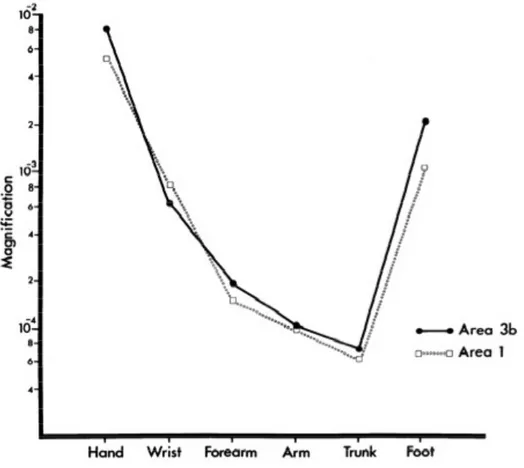
To a better understanding about the magnification effect mentioned before, I suggest to have a look at this article [ “Magnification, Receptive-Field Area, and Hypercolumn Size in Areas 3b and 1 of Somatosensory Cortex in Owl Monkeys” MRIGANKA SUR, MICHAEL M. MERZENICH, AND JON H. KAAS ], in which several features in cortical area 3b, and 1, of somatosensory cortex in monkeys, were quantitatively studied. In particular, some experiments performed in that work led to a quantification of the magnification of body regions inside the primary cortex.

DISTANCE PERCEPTION

20

The overall magnification curve is illustrated below:

Figure 1. 11 Recorded Magnification for different body regions in the MRIGANKA’s

experiment.

Cortical Magnification varies greatly across different body regions. For example, the glabrous hand, or foot representation, occupies nearly 100 times more cortical tissue per unit body surface area than the trunk, or arm representations in both areas 3b, and 1. Even if these data comes from monkey, they can be also used to study the magnification in the human body, as there are several evidence about the similarity between the monkey’s cortex, and human’s cortex. This means that if we are going to consider a square surface area of 5x5 cm on the hand, and 10x10 cm on the arm, the equivalent regions in the primary somatic sensory cortex can be obtained with this simple equation:

DISTANCE PERCEPTION

21

25 cm2 _{= skin area (hand) à cortex area (hand) = 25 cm}2 _{× 0.01 = 0,25 cm}2

100 cm2 = skin area (arm) à cortex area (arm) = 100 cm2 × 0.0001 = 0,01 cm2 The result is that the space reserved in the cortex for the hand is much bigger than that for the arm, even if the square Area considered on the skin of the arm is bigger (100 cm2_{) compared with the hand (25 cm}2_{). That is consistent with the}

homunculus concept, in which some body regions are enlarged, and other regions are reduced within the cortex.

As a consequence, the application of two stimuli on the skin surface will produce a differences in the perceive distance, as the stimulated body region varies: basically, the distance on the hand should be perceived much bigger than on the arm, just because our brain has a distorted image of our body, and the magnification of each body regions is very different (like this case). After all, as we can see in the graphic, there are some body parts wherein the magnification’s difference is low, like trunk, and thigh.

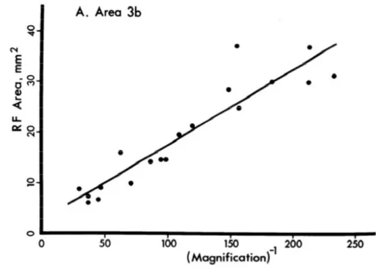
In addition, in the same study, it has been found a relationship between the receptive field size, and the amount of cortical magnification (figure 1.10). In particular, a linear relationship seems to exist between receptive field size and the inverse of cortical magnification.. Basically, regions with a high magnification (like the hands) have receptive field with a small size.

DISTANCE PERCEPTION

22

Figure 1. 12 RF Area (mm2) as a function of the inverse of the Magnification. However, focusing to the hand and to the arm, a difference in magnification equivalents to 100 times is very high, and at the same time, this kind of value is not correct to define how the Weber’s illusion could happen.

That is, the magnification concept cannot be, by itself, a complete and satisfying explanation of the Weber’s illusion. Indeed, considering only the differences in receptor density and cortical magnification, the distortion of the perceived distance across the body regions would be much more higher compared with the actual extent of Weber’s illusion. In particular, the gap between the perceived distance on the hand, and the perceived distance on the Arm, should be much more higher, if we considered only the different extension of cortical representations of the two body regions (referring to the monkey study, I should say 100 times different).

DISTANCE PERCEPTION

23

1.5.3 Green Experiment

Results of Green experiment entitled “The perception of distance and location for dual tactile pressures” support previous consideration. In one experiment Green has used the method of magnitude estimation to construct a psychophysical scale for tactile distance. In that experiment, subjects were asked to assign numbers to represent the apparent distance between two simultaneous punctual tactile stimuli. They were with eyes closed, and four area of the body exposed (palm, forearm, stomach and thigh). Each area was stimulated in both longitudinal and transversal direction. The four areas received stimulation in random sequence, and the precise location of stimulation on each area varied slightly from trial to trial. The stimuli were generated with two brass rods (contactor rods), capped with cylindrical plastic tips that were 4 mm in diameter. Stimulus distance ranged from 1 to 12 cm.

For more details consult the paper: “The perception of distance and location for dual tactile pressures” BARRY G. GREEN. Anyway, results of that experiment are shown in the figures below:

DISTANCE PERCEPTION

24

Figure 1. 1. 13 Green’s Experiment Results for four different body regions.

Thanks to this graphics, it is clear that distortions of body shape produce anisotropy in perceived distance as function of orientation. In this study, that anisotropy appears more evident on the arm than on the palm. Given the importance of this topic, and for a deeper analysis of this aspect I suggest to consult Longo’s article titled “Weber’s Illusion and Body Shape: Anisotropy of Tactile Size Perception on the Hand”.

Now, focusing on the graphics concerning the hand and the arm, we can assert that the perceived distances for the two body regions are different:

• 4 cm on the Arm = 2 perceive point. • 4 cm on the Palm = 3 perceive point.

DISTANCE PERCEPTION

25

These results verify the existence of tactile spatial distortions that were first reported by Weber. But this difference is not as high as the difference in the cortical magnification of the two body regions. Considering only differences in cortical magnification, the difference between the two perceived distances should be much bigger.

So, we can confirm that the magnification plays a key role in the Weber’s Illusion, because sets a distortion in terms of extension of cortical representation inside the primary cortex, but for sure is not the unique process. We hypothesize that there must be present other processing of tactile information that performs a sort of “rescaling”; this rescaling process, may act by decreasing the huge initial gap due to the different cortical magnification, still providing only a partial compensation (the final result is the Weber’s illusion). The neural mechanisms underlying the Weber’s illusion are still largely unknown.

1.6 The neural network and the simplifying assumptions

In this thesis, I developed a neural network model that aspires to contribute to clarify the neural mechanisms producing Weber’s illusion. Some hypotheses have been considered in model implementation; the main hypothesis is that the process of perceived distance involves two layers in the brain. The first one may correspond to the Primary Somatic Sensory Cortex, which receives inputs from the skin surface, wherein we can observe the effect of “Cortical Magnification” . The second layer, linked with feed-forward synapses to the first one, is a higher-level area: it enables to implement a sort of rescaling about the perceived distance, that partially compensates the huge effect resulting from cortical magnification. See the scheme below:

DISTANCE PERCEPTION

26

Figure 1. 14 Neural Network Scheme.

In particular, in this thesis I have developed a model (implemented in the MATLAB environment) that simulates how the brain can interpret the distance between two punctual stimuli on the skin surface of two different body regions, like hand and arm. Obviously, this solution encloses also the rescaling process mentioned before. The details of this model will be given in the next chapters.

Until now, I always talked about distance and perceived distance, but a question arises: how can the brain read out the distance between two different points on the skin surface, from neural activation in the cortex? This is still an open question. It is clear that this is a key point for the development of this thesis. In the model, we adopted a simplify solution to read distance from neural activation. Of course, we are used to think about the distance in terms of meter, centimetre, millimetre, etc., but these measure units are only a concept that we have learned with the school, and with the life experience. The real problem is to understand how the brain can associate these concepts of distance, with the effective process of elaboration distance that involves neurons inside our cortex. For the sake of simplicity, in the model, the distance between two points is

DISTANCE PERCEPTION

27

interpreted in terms of the number of inactivated neurons between two excited populations of cortical neurons (activated by two punctual tactile stimuli). This chapter is conceived as an introduction, entering the main problem faced by this thesis work. In the next Chapters, I will describe the mathematical model used to simulate Weber’s illusion.

MATHEMATICAL MODEL

2.1 Qualitative description of the model

2.1.1 The two main layers

The model aims to reproduce the main steps inside the cortex leading to the perception of distance between a pair of stimuli applied on the skin surface. To this end, two layers of artificial neurons (that may correspond to two different levels of somatosensory processing in the cerebral cortex) have been used. The main idea about this model is that the first layer could represent skin receptors plus primary somatosensory cortex neurons, and it may synthesize the property receptor density-cortical magnification of a skin region. An external tactile input directly stimulates this layer.

Suppose this first layer consists of 41 x 41 units (simulating cortical neurons), corresponding to a skin region of K x K cm (at the moment it does not matter the dimension of the represented skin region. This will be specified later). Each unit on this layer has a Receptive Field (RF) covering a specific portion on the skin surface. Since there are 41 neurons on each side of the matrix, the centres of the RFs are arranged at a distance of:

K cm / 41 neurons

A punctual stimulus, applied in a certain position, activates a “bubble” of neurons on the first layer, in particular all the neurons whose RFs cover that position.

The second layer may represent higher cortical area involved in tactile distance perception, receiving synapses from the first layer. I have assumed that this layer have the same number of units as the first layer (41 x 41 neurons). Activation of

29

the neurons within this second layer in response to an external stimulus depends on the synapses connections from the first layer. A schematic diagram of network structure is represented below.

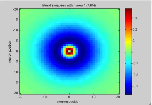
The model also includes the presence of lateral synapses within each layer (excitatory among proximal neurons, and inhibitory among distal neurons).The second layer may represent higher cortical areas that - starting from a distorted primary representation based on receptor density and cortical magnification - may partially rescale tactile information towards their true size.

The previous structure has been applied to represent two different body regions characterized by different density receptor, and cortical magnification.

• Region called A, with high-density receptors on the skin, and high cortical magnification. Supposed that this region has a dimension of 5 x 5

i = 1 i = 40 x y j = 41 j=1 j=41

First Layer = lower level of tactile processing in the cortex.

41 x 41 neurons

Second Layer = higher level of tactile processing in the cortex.

41 x 41 neurons

i = 1

i = 40 j=1

30

cm on the skin surface, and it is mapped by a matrix of 41 x 41 neurons in the cortex. In addition, each neuron has small RF size.

• Region called B, with low-density receptors on skin, and low cortical magnification. Supposed that this region has a dimension of 10 x 10 cm on the skin surface, and it is mapped by a matrix of 41 x 41 neurons in the cortex.. In addition, neurons in this area have large RF size.

Region A could be associated with the hand, whereas region B with the arm. Indeed the number of neurons devoted to each region is the same, but in the region A, 41 x 41 neurons correspond to a skin Area of 25 cm2 , whereas in region B they cover an Area of 100 cm2 _{Hence, Region A has a higher resolution}

compare with region B . In particular, the spatial resolution of neurons for the two regions is:

Ø REGION A (HAND):

5 cm / 41 neurons = 0,125 cm (the first neuron is centered in 0 cm and the last neuron is centered in 5 cm). Ø REGION B (ARM):

10 cm / 41 neurons = 0,25 cm (the first neuron is centered in 0 and the last neuron is centered in 10 cm).

Figure 2. 1 Example: Cortex Area of 41 x 41 neurons codifies for a skin region of 5

x 5 cm.

In Region A, the centers of neuron RFs are arranged at a distance of 0,12 cm whereas in Region B, the centers of neuron RFs are arranged at a distance of 0.24 cm. Moreover, RFs of neurons in the first layer have been assumed smaller in Region A than in Region B. Therefore, we can assert that Region A (Hand)

31

has higher acuity in discriminating the presence of two nearby stimuli. Instead the arm acuity will be lower.

To summarize, the first layer of this model accounts for cortical magnification that occurs in the primary somatosensory cortex: indeed, in this first layer, Region A is represented by a higher number of neurons having smaller RF, whereas Region B is represented by a lower number of neurons having larger RFs. That is, this layer gives rise to a strong distorted representation. The second layer has been included to restore, at least, partially a more truthful representation

2.1.2 Application of two punctual stimuli : effects within the first

layer

Once defined the main structure of the model, suppose to apply 2 punctual stimuli at the same distance (2.5 cm), on the skin surface of both regions. For simplicity, let’s think along one dimension (for example assume that we stimulate units along a row of the matrix showed in figure 2.1).

Example of stimulation: Region A:

The red arrows represent two punctual stimuli applied on the skin surface; these two stimuli stimulate neurons inside the first layer. In this case, the first stimulus is applied on the neuron in position 8 (j=8, RF center = j*0.125 cm = 1 cm), whereas the second one on the neuron in position 28 (j=28, RF center = j*0.125 = 3.5 cm). Each punctual stimulus creates a pattern of neurons activation (like a bubble), because there is overlap among Receptive Fields. Hence, the most

i = 20

32

excited neurons will be the eighth and the twenty-eighth, but also their neighbors will be activated, even if with a less strength.

Therefore, the pattern of neuron activation along the 20th lines of the matrix (first layer), should be like this:

Figure 2. 2 Peaks of activation along the 20th lines of the neurons matrix (Area 1, HAND).

Notice the distance between two peaks: 20 neurons. Region B:

The units are design bigger just to remember that this region has less resolution. Hence, with the same distance of 2.5 cm the 2 most excited should be much closer. For example the first stimulus will hit the neurons number 14 (j=14, RF center = j*0.25 =3.5 cm ), whereas the second one will hit the neuron number 24 (j=24, RF center = j*0.25 = 6 cm). The expected activation of neurons in that row is something like this:

Figure 2. 3 Peaks of activation along the 20th _{lines of the neurons matrix (Area 1,}

ARM). 1 2 3 4 5 6 7 8 9 10 11 12 13 14 15 16 17 18 19 20 21 22 23 24 25 26 27 28 29 30 31 32 33 34 35 36 37 38 39 40 0 0.2 0.4 0.6 0.8 1

position of neuron in the first layer (j)

neur on ac tiv at ion 1 2 3 4 5 6 7 8 9 10 11 12 13 14 15 16 17 18 19 20 21 22 23 24 25 26 27 28 29 30 31 32 33 34 35 36 37 38 39 40 0 0.2 0.4 0.6 0.8 1

position of neuron in the first layer (j)

neur on ac tiv at ion i = 20 j = 40 j = 24 j = 14 j = 1

33

With the same pair of stimuli applied at the same distance of 2.5 cm , the distance between the 2 peaks is decreased (10 neurons) due to the different resolution associated with the two regions.

Notice that on this example we are considering only the first layer, which - as we have assumed -, it is involved in cortical magnification. In fact the difference of the distance between two peaks in Region A is higher than Region B:

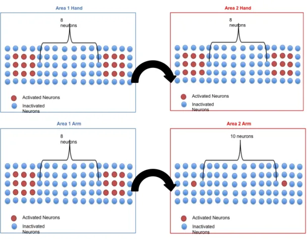
• REAGION A (HAND) : Gap within First layer = 20 neurons ; • REAGION B (ARM) : Gap within First layer = 10 neurons ; The ratio between the gaps is:

20 neurons /10 neurons = 2

so, for the same pair of stimuli, the distance in Region A is represented in the first layer as double than the distance in Region B. This is consistent with the concept of cortical magnification, as we had considered two body regions with a different cortical magnification, like Hand and Arm.

2.1.3 Application of two Punctual Stimuli: Effects Within the

Second Layer

Basically, in this model, the role of the second layer is to implement the rescaling process, in order to decrease the ratio calculated before.

The way to reach this target is to create a pattern of feed-forward synapses connections from Layer 1 to Layer 2 able to bring down the ratio with the activation and inhibition of neurons groups. The easiest solution would be decrease the gap between 2 peaks inside region A (Hand: high resolution), and increase the gap inside region B (Arm: low resolution). However, this solution seems to be not convenient, because it would lead to a resolution decrement in region A.

34

Therefore, it should be better a different implementation; as long as we want to maintain the high resolution of the region A (Hand) , it is much more convenient to work only by incrementing the resolution of the region B (Arm).

Hence, I have hypothesized that the brain implements the rescaling process by increasing the resolution of the lowest resolution region (region B in this case). At the same time, the high resolution of the region A presents in the first layer, will be kept also in the second layer too.

It is clear that to implement such kind of process, the synapses within the network concerning Region A will be different (in terms of parameters) from the network concerning Region B.

Continuing with the example, if we suppose that the rescaling process is going to increase the gap in the second layer of the region B, from 10 neurons to, for example, 14 neurons (and considering for region A that the second layer has the same gap of the first layer), the ratio becomes:

• REAGION A (HAND) : Gap within Second layer = 20 neurons ; • REAGION B (ARM) : Gap within Second layer = 14 neurons ;

RATIO = 20 neurons /14 neurons = 1.42

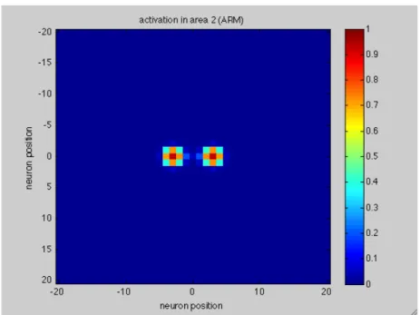
Figure 2. 4 Peaks of activation along the 20th line of the neurons matrix (Area 2, HAND)

Figure 2. 5 Peaks of activation along the 20th _{lines of the neurons matrix (Area 2,}

ARM) 1 2 3 4 5 6 7 8 9 10 11 12 13 14 15 16 17 18 19 20 21 22 23 24 25 26 27 28 29 30 31 32 33 34 35 36 37 38 39 40 0 0.2 0.4 0.6 0.8 1

position of neuron in the second layer (j)

neur on ac tiv at ion

35

Therefore, the illusion is still present, but now, on the second layer, the perceived distance is more similar across the two regions, with respect to what occurs in the first layer. That is, representation in the second layer is more truthful, since actually the distance applied externally is the same. That is, the second layer partially rescales the distortion occurring in the first layer, by reducing the difference in the perceived distance. So, in this model, the fundamental hypothesize is that the second layer (higher cortical level) of each body regions plays a key role in the perception of distance about two stimuli.

2.2 Mathematical description of the network

Since the networks representing Region A and Region B, has the same structure, only the equations for the Hand region will be presented. However, the two networks differ for the parameter values of some synapses. Hence, after description of network structure, I will emphasize the difference in parameter values between the two Regions.

The superscripts f, s will denote quantities concerning the first layer (Area 1) and the second layer (Area 2) respectively. The superscripts H and A will indicate the Hand (Region A) and the Arm (Region B). Finally the subscripts ij, hk will represent the spatial position of an individual neuron.

Each layer can be thought as a matrix of neurons. In the model, each layer is composed by N x N neurons with N = 41. The dimension of this matrix is the same for both regions. For Region A, this Area (matrix) corresponds to a skin region on the hand of 5 x 5 cm. Instead in Region B, this Area (matrix) is relative to a skin region on the arm of 10 x 10 cm.

To replicate the different resolution, RF’s centers are arranged at a distance of 0.125 cm on the Hand, and 0.25 cm on the Arm,.

In the following, I will denote with xi and yi the center of the RF of a generic

neuron ij. By considering a reference frame rigidly connected with the Hand, we can write:

36

xi = -2.625 cm + i ⋅ 0.125 cm ( i = 1, 2, …. , N) (2.1)

yj = -2.625 cm +j ⋅ 0.125 cm (j = 1, 2, …. , N) (2.2)

The same formula can be used for the Arm:

xi = -5.25 cm + i ⋅ 0.25 cm ( i = 1, 2, …. , N) (2.3)

yj = -5.25 cm + j ⋅.0.25cm (j = 1, 2, …. , N) (2.4)

Hereinafter, the RF will be denoted with the symbol Φ (receptive field). The RF of the cortical neurons in “Area 1” is described with a Gaussian Function. Therefore, for a neuron ij in “Area 1” the following equation holds:

!

(x, y) = !

" exp #

(x # x

)

+ (y # y

)

2 " (!

₎

$

%

&&

'

(

))

coordinates (still relative to the skin surface), and !0 s

and !!

s _{, represent the} amplitude and the standard deviation of the Gaussian Function (three standard deviation approximately cover the overall RF). According to the equation, an external stimulus applied at the position (x,y) excites not only the neuron centred in that position, but also the proximal neurons with RFs covering that point.

2.2.1 First layer of neurons (Area 1)

The total input received by a generic neuron ij in “Area 1” is the sum of two contributes:

• The contribution due to the external stimulus applied on the skin (called !ij(t) ).

• The contribution due to the lateral synapses, linking the neuron with other neurons within the same “Area 1” (called !ij(t) ).

37

The input that reaches the neuron ij in presence of an external stimulus, is calculated as the product of the strength of the stimulus and the receptive field, according to this equation:

!

(t) =

!

"

"

(x, y)# I

(x, y, t)dxdy

!

"

#

#

(x, y)$ I

(x, y, t)%x%y

Where If ,H _{is the external stimulus applied on the skin (Hand or Arm) at the} coordinates (x,y) at the time t. The right side of the equation (num. 2.6) means that the integral is computed with the histogram rule !x = !y = 0.0312cm .

In this model the external stimulus is reproduced as a two dimensional Gaussian Function (like a circular point):

I

(x, y, t) =

0,

t < t

I

! exp "

(x " x

₎

+ (y " y

₎

2 ! (

!

₎

#

$

%

&

'

(,

t > t

)

*

+

+

,

+

+

Where t0 is the instant of stimulus application, (x0, y0) is the central point of the stimulus, and I0

f ,H

and !I

f_{, are the amplitude, and the standard deviation of the} stimulus, respectively. I have used a small standard deviation to simulate a punctual external stimulus (see Table).

In this model the application of 2 external stimuli is simulated, applied at the same time in 2 different positions. Hence, the application of 2 stimuli is represented by the following equation:

38

I

(x, y,t) =

0,

t < t

I

!exp "

(x " x

)

+(y" y

)

2!(

!

)

#

$

%

&

'

( + I

!exp "

(x " x

)

+(y" y

)

2!(

!

)

#

$

%

&

'

(, t > t

)

*

+

+

,

+

+

!

(t) =

L

!

!

"

"

(t),

l = f , s.

(t) represents the activity of the neuron in position (h,k) inside “Area 1”, and it is a variable state. Ll,H_{ij,hk is the strength of the synaptic connection from the} pre-synaptic neuron (h,k), to the postsynaptic neuron at the position (i,j). These synapses are symmetrical and are organized as a Mexican Hat function (excitation among nearby neurons, and inhibition among distant neurons). The equation implementing Lateral Synapses is valid for the first layer, as well as for the second layer:

!!,!_!",!! = !!,!_!" ∙ exp −(!! !,!_!! ! !,!₎!_!(! !!,!!!!!,!)! !∙ !_!!"!,! !            −!!,!_!" ∙ exp −(!!!,!!!!!,!)!!(!!!,!!!!!,!)! !∙ !_!!"!,! ! ,      !" ≠ ℎ!            0,      !" = ℎ!       (2.10)

l = f , s.

xi and yj represent the position of the post-synaptic neuron within the “Area 1”

and xh, yk represent the position of the presynaptic neuron within Area1. Lex l,H

and !_!!,!_!" define the Excitatory Gaussian function, whereas parameters Lin l,H _and

!_!!,!_!" the Inhibitory one. To implement a correct Mexican Hat function, some

conditions have to be satisfied:

39

!

<   !

     ! = !, !

The null term in equation (num. 2.10), avoids the auto-excitation. Finally, the total input, called uij

f ,H

(t) received by a cortical neuron in “Area 1”

(First Layer) is the sum of the two contributes:

u

(t) =

!

(t) +

"

(t)

The neuron activity is computed from its input through a first order dynamics (simulation of the passage through the neuron’s membrane), and a static sigmoidal relationship (simulation of the neuron answer):

!

= −!

_{! + !(!}

!  ),

! !

!

=

 . (2.15)

Where !_!"!,! ! is the state variable representing neuron activity. Function ! !_!"!,! ! represents the sigmoidal function of the neuron.

40

The parameter is the value of the input at the central point (that is the value of the input at which activity is equal to Gmax/2; is the slope of the sigmoid at the central point, and is the upper saturation value of the sigmoid, that is the maximum activity value for a generic neuron. Gmax has been set equal to 1, so that neuron activity is normalized with respect to its maximum. According to previous equation (num. 2.15), the activity of a generic neuron inside “Area 1” is equal to zero until its total input is under a given threshold. ! is the time constant of the differential equation (num. 2.14).

Differential equation (num. 2.14) is implemented numerically with the Euler’s method:

!

=   !

+ ℎ ∙ ! !  ,  !

,      ℎ =

. (2.16)

!

=   !

+  

∙ −!

+  

!!!"#  (!!∙(!_!"!,!!!_!!,!)

(2.17)

As long as T is the time length of the simulation, and P is the number of subdivisions of T, it is clear that h represents the sampling step of the Euler’s method.

2.2.2 Second layer of neurons (Area 2)

The Second Layer (Area 2) is assumed to be associated with a high cortical layer. In this model, neurons inside this area, receive inputs from:

• Neurons in “Area 1” via Feed-Forward synapses, having a Mexican Hat distribution.

• Neurons of the same Area via Lateral Synapses, having a Mexican hat distribution.

The following equations hold:

(2.18) u0 f k Gmax

u

(t) = !

(t) +

!

(t)

41

!

(t) =

W

"

"

#

!

_(t),

(t) represents the activity of the neuron hk in “Area 1”. W_ij,hkf ,H _{denotes the} feed-forward synaptic strength from the pre-synaptic cortical neuron hk in “Area 1”, to the post-synaptic neuron ij in “Area 2”. These synapses can be described as follows: !_!",!!!,! =  !_!"!,! ∙ exp −(!!!,!!!!!,!)!!(!!!,!!!!!,!)! !∙ !_!!"!,! ! +       −!_!"!,!∙ exp −(!!!,!!!!!,!)!!(!!!,!!!!!,!)! !∙ !_!!"!,! !         (2.20) Where xi s,H_, yj

s,H_{, represents the position of the ij neuron in “Area 2”, and}

xh f ,H_,

yk

f ,H_{, the position of the neuron hk in “Area 1”. Notice that when the coordinates} of these two neurons are equals, the exponential term assumes an unitary value, and then the synapse connection between these two neurons has the strongest value.

The activity of a neuron in “Area 2” can be computed from its input with the same equation as before (num. 2.14):

!

= −!

_{! + ! !}

! ,

! !

!

=

 .

k is the slope of the sigmoid at the central point, is the value of the input at the central point, and is the gain of the sigmoidal function.

It can be solved by Euler’s method:

!

=   !

+ ℎ ∙ ! !  ,  !

     ℎ =

!

=   !

+  

∙ −!

+  

. (2.24)

42

As long as T is the time length of the simulation, and P is the number of subdivisions of T, it is clear that h represents the sampling step of the Euler’s method.

2.3 Parameters and their values

Lex f ,H = 1 Lin f ,H = 0.5 !ex f ,H = 2 neurons !in f ,H = 8 neurons Lex f ,A = 1 Lin f ,A = 0.5 !Lex f ,A = 2 neurons !Lin f ,A = 8 neurons Feed-Forward Synapses Wex f ,H = 4 Win f ,H = 1 !Wex f ,H = 1 neurons !Win f ,H = 1.4 neurons W_exf ,A = 4 W_inf ,A = 1 !Wex f ,A = 1 neurons !Win f ,A = 1.4 neurons

Lateral Synapses in Area 2 Lex s,H = 4.5 Lin s,H = 2 !ex s,H = 1.5 neurons !in s,H = 2 neurons Lex s,A = 4.5 Lin s,A = 2 !ex s,A = 1 neurons !in s,A = 2 neurons Sigmoidal characteristic Gmax= 1 k = 0.6 u f 0 = u s 0= 12 Time constant ! = 3 ms