ALMA MATER STUDIORUM - UNIVERSITÀ DI BOLOGNA
CONSEIL EUROPÉEN POUR LA RECHERCHE NUCLÉAIRE - CERN (CH)
SCUOLA DI INGEGNERIA E ARCHITETTURA
DIPARTIMENTO DI INGEGNERIA DELL’ ENERGIA ELETTRICA E DELL’INFORMAZIONE
“GUGLIELMO MARCONI” - DEI
CORSO DI LAUREA MAGISTRALE IN INGEGNERIA ENERGETICA
MASTER THESIS
in
Engineering of Superconducting Systems
Analysis of impregnated Niobium-Tin coils for the
High-Luminosity LHC magnets
Candidate:
Coordinator:
Giovanni Succi
Prof. Ing. Marco Breschi
Advisors:
Dr. Arnaud Devred
Dr. Luca Bottura
Prof. Ing. Sandro Manservisi
Ing. Enrico Felcini
Anno Accademico [2017/18]
Sessione III
A Graziella Sarti
e
A mia nonna
“Success is not final, Failure is not fatal: it is the courage to continue that counts”
Sir Winston S. Chuchill
i
Sommario
Il progetto ad alta luminosità dell’LHC prevede l’utilizzo di una nuova tecnologia di magneti
superconduttivi, che faranno affidamento su un materiale mai utilizzato in precedenza, il Nb
3Sn.
Alcuni magneti dipolari verranno sostituiti all’interno dell’acceleratore per migliorare il sistema di
collimazione dei fasci e saranno in grado di produrre campi magnetici nell’ordine dei 12 T, contro gli
8 T della macchina attuale.
La fragilità del Nb
3Sn richiede una fase di impregnazione con resina epossidica durante il processo
produttivo degli avvolgimenti, per evitare che si verifichi lo spostamento relativo dei fili causato dalle
forze di Lorentz, che provocherebbe uno sforzo eccessivo su di essi, degradandone le proprietà
superconduttive. Allo stesso tempo, l’impregnazione impedisce all’elio superfluido, il liquido
refrigerante, di filtrare all’interno degli avvolgimenti, causando una sostanziale differenza nel
comportamento termico delle bobine rispetto a quelle realizzate in Nb-Ti.
Alcune prove sperimentali sono state condotte presso il laboratorio di criogenia del CERN per
studiare il comportamento termico di un campione del dipolo dell’11 T sottoposto a perdite AC, con
valori tipici di densità di potenza nell’ordine del 𝑚𝑊/𝑐𝑚
3. Il campione veniva inserito all’interno di
un contenitore isolante, in cui solamente la superficie dello strato interno di conduttori rimaneva
esposta all’ambiente esterno. Il tutto veniva poi immerso in elio superfluido, per rappresentare al
meglio la situazione reale.
Questa tesi, che è stata svolta presso il gruppo MSC (Magnets, Superconductors and Cryostats) del
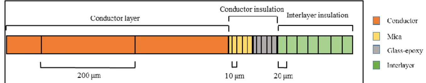
CERN, è incentrata sullo sviluppo di un modello 1-D di una linea radiale giacente sul piano di
mezzeria di un quadrante del magnete. Esso è anche rappresentativo dei materiali della sezione ed è
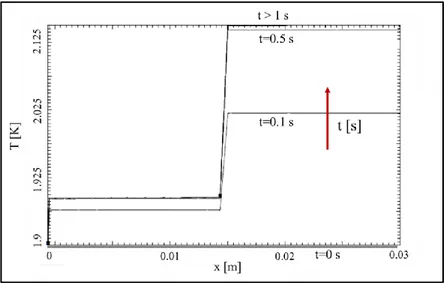
stato utilizzato allo scopo di studiare l’evoluzione di temperatura e i profili stazionari in risposta a
introduzioni di calore nei conduttori, simili a quelle dell’esperimento citato.
Lo stesso modello è stato poi adattato al caso di prove di quench eseguite presso la SM-18 facility su
modelli corti del dipolo dell’11 T. In tali test, riscaldatori induttivi venivano energizzati per rilasciare
calore nel magnete, in modo che il quench venisse innescato a partire da certe condizioni operative
di corrente e campo.
Partendo dalle mappe di campo e dalla parametrizzazione per il materiale superconduttivo, è stato
possibile ricavare i valori di 𝑇
𝑐𝑠, usando di fatto il magnete come un sensore di temperatura.
Il lavoro presenta una descrizione dettagliata del modello e delle ipotesi fatte per condurre le
simulazioni, insieme ad una sua validazione tramite il confronto con le suddette prove sperimentali.
ii
Abstract
The High-luminosity project of the LHC calls for the employment of a new technology of
superconducting magnets, which will make use of a material never used before, Nb
3Sn. Some of the
dipole magnets will be replaced inside the accelerator to enhance the collimating system of the beams
and will be capable of producing magnetic fields in the order of 12 T, against the 8 T of the present
machine.
The fragility of Nb
3Sn requires an impregnation stage with epoxy resin during coil manufacturing, to
avoid that relative movement between strands takes place due to Lorentz forces, which would be the
source of excessive stress on strands themselves, degrading their superconducting properties.
At the same time, the impregnation prevents superfluid helium, the liquid coolant, from filtering
inside the coils, thus causing a substantial difference in the thermal behavior with respect to Nb-Ti.
Experimental tests were conducted at the cryogenic laboratory at CERN to study the thermal behavior
of a sample of the 11 T dipole under AC losses, with typical values of the input power density in the
order of the
𝑚𝑊/𝑐𝑚
3. The sample was inserted into an open box of insulator, with the surface
corresponding to the inner layer of conductors being the only one exposed to the exterior, and was
then immersed in superfluid helium, to get closer to real operation.
This thesis, which was carried out at the MSC (Magnets, Superconductors and Cryostats) Group at
CERN, regards the development of a 1-D model of a radial line crossing the middle plane of a
quadrant of the magnet. It is also representative of the materials in the section and it was used with
the aim to study the temperature evolution and steady-state profiles in response to heat injections in
the conductors, similar to those provided in the experiment.
The same model was adapted to reproduce results of quench tests carried out at the SM-18 facility on
short models of the 11 T dipole. In such tests, inductive heaters were energized to release heat in the
magnet, in order to trigger the quench phenomenon, starting from given operating conditions of
current and field. Using magnetic field maps together with the parametrization of the superconducting
material, it was possible to derive local values of the 𝑇
𝑐𝑠, thus employing the magnet as a temperature
probe.
This work presents a detailed description of the model and of the hypothesis made to run the
simulations, together with its validation obtained through the comparison with experimental tests
cited above.
iii
Introduction
The mission of CERN (European Council for Nuclear Research) is aimed at fundamental research, with a special focus on particle physics. Here, between the years 2001 and 2008 the biggest and most powerful particle accelerator in the world, the Large Hadron Collider (LHC), was built. This accelerator is capable of colliding hadron beams (protons or lead ions) at an energy never reached before, namely 14 TeV in the center of mass, which enables to study the moments immediately following the Big Bang.
The employment of this machine and of its four big detectors has brought, at the present day, to important achievements, as the discovery of the Higgs boson and the demonstration of the existence of penta-quarks. Despite accomplishments in particle physics are of major relevance for the outside world, it is important to consider that a machine so complex as the LHC requires considerable efforts from an engineering point of view. Many systems are involved to obtain proper operation of the machine, from superconducting magnets to cryogenics, from radiofrequency cavities up to kicker magnets, used for injection and extraction of the beams from the machine. Furthermore, the LHC is only the final stage of an entire complex of accelerators, some of them dating back to the establishment of the center.
An upgrading project of the machine, called High-Luminosity LHC, is planned to be completed by the year 2025, which will bring the luminosity, a key parameter for particle physics, a factor ten higher with respect to the present value. This will enable to gather much more data on particle collisions, increasing the potential of discovery of new fundamental phenomena. The fulfillment of such project requires the substitution of some dipoles and of 16 quadrupoles inside the machine, with new versions that will make use of Nb3Sn coils, a superconducting material never used before to build accelerator magnets, which will enable to increase magnetic fields to 12 T, a considerable advance with respect to the 8 T provided by the present material, Nb-Ti.
Nb3Sn requires a special process of fabrication, at the end of which a very fragile composite is obtained, due to the crystalline structure which characterizes this intermetallic compound. Coils are then impregnated using epoxy resin in a way that displacements between adjacent strands are blocked, thus avoiding excessive degradation by mechanical stresses. Determining the thermal behavior of this new technology of magnets is fundamental for their future employment in the machine, since they are significantly different from the past. The aim of this work is to present a thermal study on the dipole magnet for the High-luminosity project (also named “11 T”), where a 1-D model was developed in order to reproduce the features of the magnet under examination. The HEATER software was used for this purpose [40]. This is able to solve the heat conduction equation in complex geometries and under the application of external sources, initial and boundary conditions. The complexity of the model was gradually increased to finally reproduce the proper geometry and material composition along a line radially crossing the middle plane of a quadrant of the magnet.
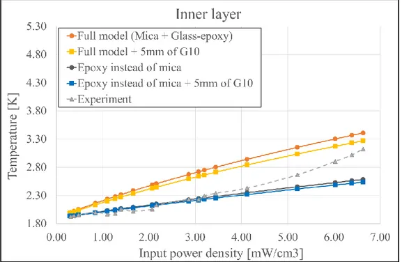
The model was used to reconstruct the temperature profile inside the magnet, both in transient and steady-state regime, in response to heat depositions in conductor layers. Such depositions were modeled as provided from the experiments carried out both at the cryogenic laboratory (Cryolab) [37] and at the SM-18 facility at CERN. Comparison with measurement results is reported.
The work opens with an introductory chapter about CERN and its purposes, where an explanation of the operation principles of accelerators is given. The accelerator complex which brings to the final stage, namely the LHC, is shown, and an outline of the features of the high-luminosity project is also displayed. A second chapter offers an overview on superconductivity, with a special focus on the technologies involved in magnets production.
The third chapter is dedicated to a presentation of the state-of-the-art concerning the mechanisms of heat exchange between the liquid coolant, helium, and superconducting cables made of Nb-Ti. The study begins from a first article [7] and then extends to a bibliographic research about heat exchange problems in a more general sense.
The main chapters present the activity which saw me involved at CERN, and which concerns subjects linked to heat exchange. The Cryolab experiment is firstly illustrated, to then pass at the 1-D simulation in HEATER. Care is adopted for the description of the approach to the problem, with a special focus in explaining all the details of the model, as the choice of the mesh, initial conditions and boundary conditions, as well. Discussion
iv
of the results is very important for the purpose of this text, since the first simulations were significantly different from experimental ones. Consequently, a serious process of revision was undertaken, making assumptions that let us obtain a much better match with the measurements. These assumptions regard the role played by materials in the system from a thermal perspective and will be adequately justified.
The same model was then used to simulate quench tests carried out on short samples of the 11 T dipole. Quench is a major problem for superconducting magnet operation, since it is linked to the stability of magnets themselves. This phenomenon is typically produced by localized heat releases, which cause the transition of a small portion of material to the normal state, with the subsequent propagation to the entire magnet by Joule effect. Inductive heaters, called quench heaters, are normally instrumented on the external radius of the magnets, to ensure a uniform heating in the case a quench is detected, and to avoid excessive extra-heating in localized points. Two kinds of tests were conducted using quench heaters. In some of them, heaters were placed as in real operation, like the one already described. In others, they were inserted in the space between the two conductor layers, substituting the interlayer. Heat deposition in the magnet caused a temperature rise in both cases, with the following trigger of a quench. An interesting aspect is that the knowledge of operating conditions of the magnet and of the critical curve makes, to a certain extent, the magnet as a temperature probe. The 1-D model was adapted to the respective geometries cited above, to understand if it was able to reproduce, firstly, quench detection in the same blocks identified in the measurements and, secondly, in the inner layer of the coil, which sees the higher values of magnetic fields. We started from field maps computed using the ROXIE software, to derive the field profiles on radial lines considered the most critical ones. Next, the Nb3Sn parametrization for ITER [38] was used, conveniently modified for the cables of the 11 T dipole, and to derive the current sharing temperature profiles, 𝑇𝑐𝑠, along the same lines. The criterion defined to determine quench
initiation was the overtaking of the temperature profile coming from the simulation with respect to the one coming from the 𝑇𝑐𝑠, as in the computations above. A comparison with experimental results is presented, together with their interpretation.
In parallel with these two main studies, another one was performed, which is reported in Appendix I, aiming at determining the effective thermal conductivity of impregnated Rutherford cables made of Nb3Sn.
Computations were made along all the three dimensions of the cable, and it was shown how the strand twisting plays a significant role in rising the conductivity along the major direction of the cable cross-section. In fact, strands behave as tubes for heat transmission, being made of more than 50% of copper. In this last case, results were compared again with experimental measurements on coil samples [34], performed along the radial and azimuthal direction of the coils. Explanation for discrepancies between analytical computations and experimental results is given.
v
Contents
1. CERN and the Large Hadron Collider 1
1.1 CERN and its aim……… 1
1.2 The synchro-cyclotron and accelerators operation………..………... 1
1.3 The CERN accelerator complex………..………... 2
1.4 The High luminosity LHC……… 4
2. Superconductivity 6
2.1 Introduction and historical background……… 6
2.2 Perfect diamagnetism (Meissner effect)……..……… 8
2.3 Critical parameters of superconductors………. 10
2.4 Type I superconductors………..……….. 11
2.5 Type II superconductors……….. 11
2.6 Theories of superconductivity………..……… 12
2.7 High Temperature Superconductors (HTS)……… 13
2.8 Technologies for superconducting materials…..………..……….……… 15
2.8.1 Niobium-Titanium………...……… 15
2.8.2 Niobium-Tin…...………...……..………. 15
2.8.3 Fabrication methodologies of Nb3Sn strands……….. 16
2.8.4 Cables and coils for accelerator magnets…………....……… 17
2.9 Comparison with Nb-Ti cables……… 19
3. Heat exchange properties of Helium in
Nb-Ti superconducting cables 21
3.1 Heat loads during machine operation………..……… 21
3.2 The quench phenomenon……….……….……….. 21
3.3 Introduction to the model…..…….………..……….………. 22
3.4. Heat transfer to helium……… 24
3.4.1 ℎ𝐾 (Kapitza)……..……… 24 3.4.2 ℎ𝐵𝐿 (Boundary layer)….……….………..………. 25 3.4.3 ℎ𝑆𝑆 (Steady-state)….……….………...……… 26 3.4.4 ℎ𝐻𝑒𝐼 (Helium I)……….……… 28 3.4.5 ℎ𝑛𝑢𝑐𝑙.𝑏𝑜𝑖𝑙.(Nucleate boiling)……..………..………... 29 3.4.6 ℎ𝑓𝑖𝑙𝑚 𝑏𝑜𝑖𝑙. (Film boiling)………….………... 31 3.4.7 ℎ𝐻𝑒𝐼(Gaseous helium)…….………….………. 32
4. The Cryolab experiment 33
4.1 Introduction……… 33
4.2 The experiment………... 33
4.3 A brief outline about AC losses……….……….. 33
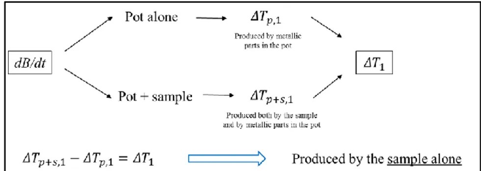
4.4 The calibration procedure……….……….. 37
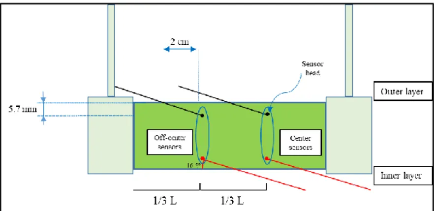
4.5 Temperature measurements and sensors mounting……….……… 39
vi
5. Numerical model and simulation results 44
5.1 Introduction………. 44
5.2 The Cryolab experiment model………... 45
5.3 Mesh……… 47
5.4 Initial and boundary conditions………….……….. 47
5.4.1 Initial conditions……….. 48 5.4.2 Boundary conditions……… 48 5.5 Heat inputs……….. 49 5.6 Temperature comparison……… 50 5.7 Simulation results………... 51 5.8 Analytical validation………... 52
5.9 Analysis of the results………. 55
5.10 Time constants……….. 58
5.11 Discussion of the results………. 58
5.12 A first consideration……….. 60
5.13 The fall of the adiabatic condition……… 62
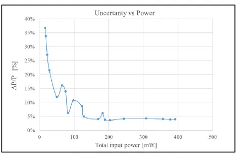
5.14 Some other comparisons: the error bands………. 63
5.15 Heating distribution……… 66
5.16 The sign of the second derivative……….. 68
5.17 A possible explanation………. 70
5.18 A resume of the approach………. 71
5.19 AC losses computation……….. 71
6. Tests at the SM 18 facility 72
6.1 Introduction………. 72
6.2 Geometry of a quench heater……….. 72
6.3 Boundary conditions……… 73
6.4 Outer layer quench heater tests………. 73
6.5 Interlayer quench heater tests……….. 75
7. Conclusion 82
Acknowledgement 83
Appendix I. Effective thermal conductivity of Nb
3Sn impregnated Rutherford cables 84
A.I.1. Rutherford cables……… 84
A.I.2. Assumptions of the study and definitions……….………... 85
A.I.3. Local and global reference systems……… 86
A.I.4. Computations……….. 88
A.I.4.1. Thermal conductivity along the y’ axis……….………… 88
A.I.4.1.1. Copper fraction in a strand……….………. 89
A.I.4.2. Thermal conductivity along the x’ axis……….……… 90
A.I.4.3. Thermal conductivity along the z’ axis……….……… 96
A.I.4.4. Tensor rotation and effective thermal conductivity...………. 96
A.I.4.5. Thermal conductivity on a multiple twist-pitch scale…...………. 98
A.I.4.6. Comparison with experimental measurements……….100
Appendix II. Volume of metallic parts of the Cryolab sample 104
Appendix III. Detailed data about the experiments 105
1
1. CERN and the Large Hadron Collider
1.1 CERN and its aim
CERN, acronym for Conseil Européen pour la Recherche Nucléaire, is the European laboratory for nuclear research, created in 1954 just few years after the end of the Second World War.
The idea behind the establishment of the center, which laid in the mind of the French physicist Louis De Broglie and which was then supported by other scientists as the Italian Edoardo Amaldi, was to create a place that could gather the best minds all over Europe, in order to carry out fundamental research both in theoretical and experimental physics, while trying to stop the so-called “mind-drain” from Europe to United States, which characterized the war years.
The Convention for the Establishment of the Organization [1] states, in its Purposes, that “the Organization should provide for collaboration among European states in nuclear research of a pure scientific and fundamental character, and in research essentially related thereto. The Organization shall have no concern with work for military requirements and the results of its experimental and theoretical work shall be published or otherwise made generally available”.
These words, from which shines a crystalline purpose, derive the main activities of the center. They are basically three: 1) Provide a unique complex of accelerators and facilities to study nuclear physics; 2) Provide a strong international environment, where people from all over the world can gather, in order to push the boundaries of science and knowledge, in a general sense; 3) Deepen the study in fundamental physics, to uncover the secrets of nature and the universe.
1.2 The synchro-cyclotron and accelerators operation
The first machine to be built at CERN was the synchro-cyclotron, which at its time became the most powerful accelerator in the world, and whose construction lasted from 1955 to 1957. Its operation was based, as other accelerators, on the combination of electric and magnetic fields, which both act on charged particles. There is a substantial difference in the way electric and magnetic forces act on a particle, which is addressed in eq.(1.1)
𝐹⃗ = 𝑞𝐸⃗⃗ + 𝑞 𝑣⃗ 𝑥 𝐵⃗⃗ . (1.1)
The first term on the right-hand-side (rhs) represents the electric force, which acts in the same direction of the field, so that it makes a work on a particle. The second term, on the other hand, represents the magnetic force, which acts in the direction normal to the field, so that it does not apply a work on the particle. To resume, electric fields accelerate particles, which in turn means give energy to them, while magnetic fields can bend particles.
The machine made use of massive vacuum pumps to extract the air from the inside of its chamber, and to avoid particles to collide with air molecules. In the proton source, hydrogen gas was ionized so that their nuclei, being protons, could be injected in the middle of the synchro-cyclotron. Two D-shaped electrides with opposite polarity were fixed inside the vacuum chamber, in the middle of the external magnet. The magnet consisted of two coils, each wound with 6380 m of aluminum conductor, carrying 1800 A and dissipating a total power of 750 kW. Pole discs had a diameter of approximately 5 m and the total weight of the magnet was 2500 tonnes [2]. Protons, having a positive charge, were driven to the negative electride, starting their acceleration through the gap between the two electrides. The magnetic field forced them to follow a circular trajectory, and they returned to the gap after one-half turn. Meanwhile, the radio-frequency generator reversed the polarity of the two electrides, so that protons were now attracted to the opposite electride, continuing their path and gaining more energy. This process was repeated over and over again, and every time protons completed a half turn, the radius of their path increased. After completing more than 100.000 turns they reached an energy of 600 MeV, corresponding to 80% the speed of light [46].
The synchro-cyclotron played a fundamental role in the physics of the pion, particularly in studying its rare decays. From 1964 the machine began to focus on nuclear research, leaving particle physics to the new and more powerful proton-synchrotron. Its life went on, though, providing beams for the ISOLDE facility, dedicated to radioactive ion beams. It was finally dismissed in 1990, when the line was transferred to the proton-synchrotron booster.
2
1.3 The CERN accelerator complex.
It is worth to briefly describe the accelerator chain at CERN. The journey starts from a tiny bottle of hydrogen which, at a precise rate of 1.2 seconds, releases 1014 hydrogen atoms which go into the source chamber of a linear accelerator, LINAC 2. Here, hydrogen atoms are stripped off from their electrons, to leave hydrogen nuclei, which are protons, indeed. Having a positive charge, they can be accelerated by an electric field, and by the time they emerge they gain an energy of 50 MeV, corresponding to nearly 30% of the speed of light. They are now about to enter the proton-synchrotron booster (PSB). Started operation in May 1972, the PSB is made up of four superimposed rings. Its main function is to increase the number of protons that its next companion, the Proton-Synchrotron (PS) can accept. In fact, in order to maximize the intensity of the beam, the initial packet is divided into four, one for each of the Booster rings. At this point, a linear acceleration would be impractical, the reason why the PSB is circular, being 157 m in circumference. Protons are here also accelerated by means of a pulsed electric field, which increases the energy of the beams at each turn. As seen for the cyclotron, magnets are used to bend the particles and keep them on track. The concept of a synchrotron is that particles are bent on a fixed path, with the magnetic field increased over time, and synchronized with the energy of the beam. All accelerators we will describe from this moment on are synchrotrons.
The PSB accelerates particles up to 1.4 GeV, corresponding to 91.6% the speed of light. It also squeezes the bunched in order for particles to stay closer together. Recombining the packages from the four rings, the next step is the Proton-Synchrotron (PS), the third stage of the particle journey. The PS was the second machine inaugurated at CERN and accelerated its first protons on 24 November 1959, also becoming for a short period the world’s highest energy particle accelerator, and the first CERN synchrotron. From this type of particle accelerators comes the term “synchrotron radiation”, which is used in a wide range of applications, from geology to particle therapy. The proton-synchrotron at CERN is characterized by a circumference of 628 m, and has 277 conventional (ferromagnetic) electromagnets, where 100 are dipoles to bend the particle beams. It operates up to 25 GeV and it is a key component in the CERN’s accelerator complex.
In its early days, LINAC 2 sent particles directly to the PS. However, its low energy limited the number of protons that the PS could accept and this was the reason to build an intermediate stage, the PSB. Inside the PS, protons circulate for 1.2 seconds, reaching 99.9% the speed of light. A point of transition is reached here: energy transmitted to particles through electric fields does not translate in a further increase in particle velocity, so all the energy contributes only to increase the mass of the particles. This is well explained thanks to the special theory of relativity
𝑚 = 𝑚0 √1 − 𝑣𝑐22
.
(1.2)
In eq.(1.2) 𝑚0 is the mass of the particle at rest, v is the velocity of the particle, and 𝑐 is the speed of light. To be more precise, it is to be said that in experiments everything behaves in the same way as if the mass of
particles was increased. Despite this subtle aspect, it will make no difference, for our present purposes, to
consider that the energy increase translates in an effective increase in the mass of the particle.
It is worth to define something else before going on. The energy of the particles is commonly expressed in a unit called electronvolt, which by definition is the energy acquired by an electron moving in an empty region of space between two points which have an electrical potential difference of 1 V. An electronvolt is a tiny amount of energy, corresponding to
1 𝑒𝑉 = 1.602 ∗ 10−19 𝐶 ∗ 1 𝑉 = 1.602 ∗ 10−19 𝐽 . (1.3)
In the theory of special relativity, energy and mass are interchangeable, due to the Einstein’s relation
3
Therefore, the mass of the particles can be expressed in terms of energy, in eV/𝑐2, or eV, to be shorter.
The mass of the proton at rest is 938.27 MeV/𝑐2, almost 1 billion eV. When protons pass through the PS, they
acquire an energy of 25 GeV, equivalent to 25 times their mass at rest.
Particles from the PS are injected to the Super-Proton-Synchrotron (SPS). The SPS is the second largest accelerator at CERN, being 7 km in circumference. It began its work in 1976 and during his operation has enabled various kind of studies, from the inner structure of the proton to the investigation of the asymmetry between matter and antimatter. Its major contribution came in 1983 with the discovery of the 𝑊± and 𝑍0 bosons, which mediate the weak force, using proton-antiproton collision. That discovery was awarded with the Nobel prize in Physics to the Italian physicist Carlo Rubbia and the Dutch Simon van der Meer.
The SPS is properly designed to receive protons at 25 GeV and “accelerates” them up to 450 GeV. It has 1317 conventional (room-temperature) magnets, including more than 700 dipoles to bend the beams. When the packets are energized sufficiently, they are launched into the orbit of the Large Hadron Collider (LHC). Let’s have a look at Fig.1.1, to visualize what has been said so far.
Being one-hundred meters below ground and 27 kilometers in circumference, the LHC is the world’s biggest and more powerful accelerator. It contains two beam pipes, one circulating clockwise and the other counterclockwise. It takes 4 minutes and 20 seconds to fill each LHC ring, and 20 minutes for the protons to reach their maximum energy of 6.5 TeV. The beams collide in 4 points in the machine, where detectors are placed. They are: ATLAS, CMS, ALICE, and LHCb; the energy in the center of mass is the sum of that of the two beams, namely 13 TeV. Eq.(1.4) shows how a certain amount of energy can be converted into mass, so the higher is the energy, the higher the resulting mass can be. The reason why all the efforts during the past 60 years have been made to go higher in energy are due to this rather simple idea. In fact, as the mass which can be created is higher at higher energies, also the probability that rare phenomena can happen becomes higher. Probability is also related to luminosity, which will be explained hereinafter.
ATLAS and CMS are two general-purpose detectors, which investigate a wide range of particle physics. They were the protagonists of the discovery of the Higgs boson, announced in July 2012, which ended a 50-years race for its search. Similarly to 1983, it brought to the assignment of the 2013 Nobel prize in Physics to the British physicist Peter Higgs and the Belgian François Englert, who independently proposed the Brout-Englert-Higgs mechanism in 1964. The two detectors are also looking at the possible existence of extra dimensions and dark matter particles, in search for physics beyond the Standard Model. ALICE and LHCb, on the other hand, have different objectives. ALICE studies the properties of the quark-gluon plasma, a form of matter that is supposed to have existed at the very beginning of the Universe, few fractions of a second after the Big Bang. It has been so far observed that this mixture behaves as a very particular fluid, being 30 times denser than an atomic nucleus, but that also having zero viscosity, as a perfect fluid. LHCb, where the “b” stands for beauty
4
(after the name of the corresponding quark), is the smallest of the four detectors, and investigates the existing asymmetry between matter and antimatter.
The LHC is an outstanding machine, which represents the peak of the efforts made by generation of scientists all over the world. Despite all that LHC represents, CERN is more than that. Several other experiments are conducted there. To give some examples, the aim of the ALPHA experiment is to study the properties of anti-matter, and of anti-hydrogen atoms, in particular. One of its goals will soon be the measurement of the behavior of the anti-atoms in the Earth’s gravitational field. Another important test will be the analysis of the spectrum of the anti-hydrogen, to put the famous CPT symmetry at test. There are other wonderful pieces of science at CERN, such as nTOF, for the study of interactions between neutrons and nuclei, ISOLDE, for the exotic atomic nuclei, and the CERN Neutrinos to Gran Sasso, whose aim is to investigate neutrino properties as its changes in flavor.
1.4 The High luminosity LHC
The LHC is a synchrotron-type accelerator, which means that the magnetic field is increased over time in order to follow the energy increase of the beams. Electrical fields are used to accelerate particles, through RF cavities which operate frequencies around 400 MHz. Magnetic fields, on the other hand, have three main roles in a particle accelerator: 1) Beam bending; 2) Beam focusing; and 3) Particle detection.
The bending of the beams is achieved using dipole magnets (MB, Main Bending), while focusing is done thanks to quadrupole magnets (MQ, Main Quadrupole). Particle detectors take also advantage of magnetic fields to bend particles inside the detector itself, making it easier to reveal the charge and mass of the particles, relying on the covered path when subject to a given field.
Back in 2011, studies for the enhancement of the LHC began, which would have involved a 15-year project, whose aim was to raise the potential of discoveries of the machine after 2025. The main goal of the High-luminosity project is to increase the High-luminosity of the LHC by a factor ten beyond its first design project, enabling to gather much more statistics. This may lead to a better understanding of the 10 TeV energy scale and potentially bring to new discoveries.
Luminosity is an extremely important indicator of the performance of an accelerator, and is defined as the number of events detected, N, in a certain time, t, to the interaction cross-section, σ [3]
𝐿 = 1 𝜎 𝑑𝑁 𝑑𝑡 [ # 𝑐𝑚2𝑠] . (1.5)
In practice, L is dependent on the particle beam parameters, such as beam width and flow rate. A very important quantity is also the integrated luminosity, which is the integral of the luminosity with respect to time
𝐿𝑖𝑛𝑡 = ∫ 𝐿 𝑑𝑡 . (1.6)
Luminosity and integrated luminosity are crucial parameters to characterize a particle accelerator. The LHC has the highest luminosity with respect to all the other accelerators ever built in the world, sharing it with the KEKB in Japan, with a value of 2.1 ∗ 1034 𝑐𝑚−2𝑠−1.
The effort to be put in place to achieve luminosities ten times higher than the present values will be very demanding from a technological point of view. Several components of the machine will need replacement or
new installation, and can be summarized in the following:
- Main Focusing magnets - Main Bending magnets - Crab cavities
- Power transmission lines - Accelerator chain
5
One of the most relevant aspects consists in increasing the “squeezing” of the beams. This is put in practice using sets of quadrupole magnets. The High-luminosity project aims at the substitution of existing
quadrupoles with new generation ones, which will make use of Nb3Sn, a superconducting material which was
never used before, but which enables to reach magnetic fields much higher than the present material, Nb-Ti. New versions of the main bending magnets will also be built, using again Nb3Sn. The magnets will be shorter than in the present machine, each being 5.5 meter-long, and coupled in pairs so that 4 meters will be left to have additional space for corrector magnets, thus enabling a better control of the beams even far from the interaction regions. One single demonstrator of the so-called 11T dipole will be installed during the Long Shutdown 2 (2019-2020) and put into operation during the Run 3 (2021-2023).
Another fundamental aspect of the project are the crab cavities, an innovative superconducting equipment which will give the particle bunches a transverse momentum before meeting, thus enlarging the overlap area of the two bunches and increasing the probability of collision. Sixteen of such cavities will be installed close to the main detectors, ATLAS and CMS.
Superconducting transmission lines will connect the power converters to the accelerator. This new type of cables makes use of both high-temperature superconductors (HTS) and magnesium diboride (MgB2) superconductors, representing the very first industrial application of such materials. They are able to carry currents of record intensities, up to 100.000 amperes.
The injector chain described in Section 1.3 requires some major upgrade. LINAC 2 which has been in operation for 40 years, is going to be replaced by a more powerful linear accelerator, LINAC 4, which brings particles up to 160 MeV, becoming the first element of the accelerator chain. Other interventions are also planned on the PSB, the PS, and the SPS. Last, but not least, due to the much higher rate of radiation generated by the increase in luminosity, works of civil engineering are necessary in order to provide new underground facilities for electrical equipment (power converters).
6
2. Superconductivity
The purpose of this chapter is to give an overview on superconductivity, providing a first historical introduction and description of the main features of superconducting materials. The attention is then focused on the application of superconductivity for cables and coils production for the construction of accelerator magnets. The discussion is inspired by [5] and [44].
2.1 Introduction and historical background
Superconductivity is a special property of various materials, which can carry current under specific conditions, without any losses. The history of superconductivity began in 1908 with the work of Heike Kamerlingh Onnes, after a race that spanned all along the 19th century to reach lower and lower temperatures. During the 1870s only a few substances had not yet been liquified: oxygen, helium, nitrogen, and hydrogen, which for this reason were called “permanent gases”. The saturation temperature of some cryogenic fluids, at ambient pressure, is reported in Table 2.1.
The term “cryogenics” is usually referred to temperatures below -100° C. One of the biggest problems during the 19th century was to make vacuum in order to remove the mechanism of heat exchange by convection, which was achieved by Dewar in 1898. Ten years later, Onnes managed to liquefy helium (in a volume of 60 cm3), something of paramount importance, since it made available a cold reservoir to conduct experiments at very low temperatures. In that sense, liquid helium played the same role as the Volta pile for the electromagnetic field, which on its side made available a source of direct current.
In the same laboratory, but three years later, in 1911, studying the electrical properties of a very pure sample of mercury (Hg), Onnes observed the phenomenon of superconductivity for the very first time. To be more specific, Onnes noticed a sudden transition in the resistance-to-temperature diagram for mercury, as Fig. 2.1 depicts. The sample resistance diminished to non-measurable values, and mercury passed to a state with completely different electrical properties, unknown until that moment. Onnes decided to call it “superconducting state”.
Using the words of Onnes himself, “There is plenty of work which can already be done, and which can contribute towards lifting the veil which thermal motion at normal temperature spreads over the inner world of atoms and electrons” [4].
Table 2.1: Saturation temperatures of some cryogenic fluids.
Figure 2.1: Electrical resistivity as a function of temperature for mercury.
7
Researches have shown that 26 metallic elements and around 1000 alloys and compounds become superconducting at low temperature.
Before the discovery of superconductivity, resistivity was thought to be the sum of two contributions (Matthiessen formula)
𝜌 = 𝜌𝑇+ 𝜌𝑅 , (2.1)
where the first is due to thermal motion and the second to crystalline imperfections. Electrical resistivity in metals depends on the interactions of the conduction electrons with ions of the crystal lattice, which vibrate around their equilibrium position. As temperature decreases, the amplitude of motion of the ions and the energy given by the electrons to the crystalline lattice, does the same. At zero Kelvin, the motion stops, and the remaining energy transfer is due to the imperfections in the lattice. Consequently, an ideal crystal at 0 K would have no resistivity, while a real crystal would still have a residual 𝜌𝑅, dependent on the level of imperfections. Regarding traditional materials, one can define the RRR (Residual resistivity ratio)
𝑅𝑅𝑅 = 𝜌 (273 𝐾)
𝜌 (4 𝐾) , (2.2)
which is expressed as the ratio of the resistivity at 273 K and at 4 K, which varies significantly with the degree of purity. This can be also visualized in Fig.2.2.
In practice, the higher the purity, the less the resistivity at 4 K, and the higher the RRR is. This is what classical theories predicted about the behavior of metals at low temperature. Thanks to quantum theory, though, it was discovered that ρ could not even arrive at zero, due to Heisenberg Uncertainty Principle. That’s why helium does not become a solid even close to 0 K, and to reach that state it needs to be put under high pressures.
Despite the classical theory, some metals were discovered to behave very differently from copper: when they are cooled, their resistance decreases linearly, until a certain value of temperature, called the critical
temperature, Tc, at which it drops to non-measurable values. Such materials are called superconductors, and
the transition happens independently from the degree of purity of the crystal. The transition is actually a real phase change; it does not happen only electrically, but also thermodynamically, being a second-type transition, without any associated latent heat.
Figure 2.2: Resistivity dependence of copper from temperature and for different value of the RRR.
8 This can be observed in Fig.2.3.
It represents the ratio of the normalized specific heat, namely that of super-electrons referred to normal electrons, 𝐶𝑒,𝑠/𝐶𝑒,𝑛, versus the normalized temperature, 𝑇/𝑇𝑐 A similar behavior can be observed for magnetic
susceptibility.
2.2 Perfect diamagnetism (Meissner effect)
The absence of electrical resistivity at very low temperatures does not enable, alone, to categorize a material as a superconductor. Conventional materials have a resistivity approaching zero, as well. The key feature of superconductors is their response to external magnetic fields, which reveals their diamagnetic nature. Both for an ideal conductor and a superconductor, the Faraday law is true
𝛻⃗⃗˄𝐸⃗⃗ = −𝜕𝐵⃗⃗
𝜕𝑡 , (2.3)
while the Ohm law, also called constitutive law
𝐸⃗⃗ = 𝜌𝐽⃗ , (2.4)
is valid only for an ideal conductor. When resistivity goes to zero, no electric field is present inside the material, and in turn, there is also a constant magnetic field. This means that, cooling a sample of conductor material and inserting it into a static magnetic field, the magnetic field vector, 𝐵⃗⃗ remains zero inside the material. Conversely, if one puts the material inside the field, at room temperature, when cool down is applied, the field remains constant in the material even after removing the field. The state of magnetization of an ideal conductor does not only depend on external conditions, but also on the sequence perform to arrive at certain conditions. This is properly shown in Fig. 2.4.
Fig.2.3: The blue curve depicts the specific heat of the super-electrons compared to normal electrons.
Fig.2.4: Different behavior of an ideal conductor and of a superconductor when subject to external fields and cooling. Field always remains zero in a superconductor.
9
A superconductor, on the other hand, always presents no magnetic field (𝐵⃗⃗ = 0⃗⃗) inside it, whichever sequence of external field and cooling down is applied. Such effect of repulsion of magnetic field lines is what really distinguishes an ideal conductor from a superconductor, and it is called Meissner effect.
The Ampère law is important, as well
𝛻⃗⃗˄ 𝐵⃗⃗ = 𝜇0 𝐽⃗ . (2.5)
In fact, if 𝐵⃗⃗ is zero, then also 𝐽⃗ should be zero, the reason why shielding currents generate a magnetization only on the surface of the material. The total field inside the material can be expressed by the contribution of two factors, the external field, 𝐻⃗⃗⃗, and the magnetization of the material itself, 𝑀⃗⃗⃗
𝐵⃗⃗ = 𝜇0(𝐻⃗⃗⃗ + 𝑀⃗⃗⃗) . (2.6)
Again, if 𝐵⃗⃗ is zero, then 𝑀⃗⃗⃗ = −𝐻⃗⃗⃗, which means that the magnetization given by the material acts in the exactly opposite way of the external field. Currents flow in the first 10-100 nm layer, the reason why the magnetic field can also penetrate for a certain depth, decaying with an exponential law from the outside to the inside. This can be seen in Fig.2.5.
The layer where currents flow is called penetration depth, λ, and represents the depth at which the external induction field is able to penetrate. It is defined in a way that
𝐵𝑎𝜆 = ∫ 𝐵𝑑𝑙
+∞
0
, (2.7)
and its dependence on temperature is given by an experimental law 𝜆(𝑇) = 𝜆(𝑇 = 0)
√1 − ( 𝑇𝑇
𝑐) 4
. (2.8)
Even though for a completely different purpose, eq.(2.8) resembles in its form eq.(1.2). This means that, when 𝑇 is relatively far from the critical temperature, λ is almost unaltered with respect to its maximum value; on the contrary, as it approaches Tc it gets bigger, due to the asymptote. When the magnetic inductance penetrates
completely inside the material, then it returns to the normal state.
Fig.2.5: Field trend across the surface of a sample made of a type I superconductor.
10
2.3 Critical parameters of superconductors
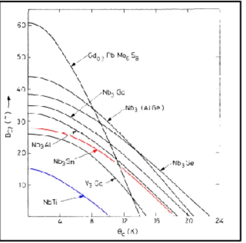
The only quantity that has been described until now is the critical temperature, which governs the transition to the superconducting state. However, there are other parameters that determine the transition, and the superconducting state is given also by current density, J, and magnetic field, B. Together, they define a critical curve, shown in Fig.2.6.
If the critical surface is cut at constant temperature, one can see the variation of Jc with B.
Fig.2.7 shows the relevant quantities in the operation of a superconductor. Drawn in red is the critical curve, at a given external field. Starting at a certain value of operating current density and temperature, 𝐽𝑜𝑝 and 𝑇𝑜𝑝,
if temperature is increased at fixed current, one arrives to cross the red curve, which means that the current sharing regime is established: the material is still superconducting, but current starts to flow also in the surrounding copper of the cable (superconducting filaments are plunged in a copper matrix which acts as a stabilizer and brings the exceeding current). At 𝑇𝑐, the material loses completely the superconducting state and
returns normal conducting. On the other hand, starting from the operation point and keeping the temperature fixed, one can increase the current until 𝐽𝑐, where the superconducting state is lost again. Unfortunately, there is no parallel for current as for the current sharing temperature as for temperature itself. Conventional conductors, like copper or aluminum, can carry around 1-2 A/mm2, arriving at a maximum of 6 using powerful cooling systems. Superconducting cables, on the other hand, can reach 500 A/mm2 (meant as an engineering current density) as it is the case for accelerator cables, thus helping to keep magnet systems compact. Finally, a fourth quantity is a critical parameter, namely the frequency. This is not normally taken into account, but can play a significant role above 109 Hz, bringing to the transition to the normal state at around 1011 Hz. The reason for this can be better understood in next sections, but it is basically related to the energy that super-electrons receive from an oscillating electric field. For all the applications we are interested in, frequency can be neglected to be a critical parameter.
Fig.2.6: Critical curve (J,B,T) for three superconducting materials.
Fig.2.7: An example of 𝑇𝑐𝑠 and Jc at a certain operating
11
2.4 Type I superconductors
Eq.(2.6) has shown that, if the magnetic field inside the material is zero, 𝐵⃗⃗ = 0⃗⃗, the magnetization generated by the material itself, by the superficial currents, is exactly the opposite of the induction field. This remains true until the critical field is reached, when a sudden transition is observed (Fig.2.8).
A high number of elements of the periodic table shows the superconducting state, between the 0.325 K of rhodium (Rh), to the 9.3 K of niobium (Nb). Most of them belongs to type I superconductors, which cannot be used to build magnets (critical fields are in the order of mT). It is important and curious to underline that common conductors are not superconductors. In other cases, it is the shape of the material to determine superconductivity (as for Beryllium), and sometimes the composition of two non-superconducting elements gives a superconductor compound. Once again, some materials become superconducting only under the effect of pressure.
2.5 Type II superconductors
In type II superconductors, the transition to the normal state does not happen with a sharp profile as for type I materials. Increasing the field, the material remains initially in a perfect diamagnetic state, until the so-called lower critical field, 𝐻𝑐,1 is reached. Here, the magnetic flux starts to penetrate inside the material, bringing it to the “mixed state”. The “mixed” region is much wider than the Meissner region, and magnetization diminishes as one approaches the upper critical field, 𝐻𝑐,2, as Fig.2.9 depicts.
In the theory by Abrikosov (which was developed in analogy to super-fluidity), the penetration of the magnetic field in the material is quantized and happens thanks to flux quanta, called vortices (𝜑𝐵 = 2.07 ∗ 10−15𝑊𝑏).
Super-currents rotate around vortices and sustain the field inside them. Fig.2.10 shows the idea. Figure 2.8: Magnetic induction B and magnetization M inside a type I
superconductor as a function of the applied magnetic field.
Fig.2.9: Magnetic induction (a) and magnetization (b) as a function of the applied magnetic field, for type II superconductors.
Fig.2.10: Simple drawing of the super-currents that support the flux inside vortices.
12
Current can easily flow around vortices, but the problem comes when their number increases. In fact, vortices repel each other, so they tend to distribute uniformly in the material, at the vertices of hexagonal structures, in order to minimize Gibbs energy.
When a current flows in the material, a Lorentz force is exerted on the vortices, which tries to make them move, originating a dissipative phenomenon (flux flow). To avoid dissipation, lattice imperfections are used to literally block the vortices, in a procedure called pinning. This can be enhanced through thermal and mechanical treatments which try to bring the average distance among imperfections close to the mean distance among vortices. If the pinning force, 𝐹𝑝 is bigger than the Lorentz force, 𝐹𝐿, vortices remain blocked, but as soon as the two forces are the same, vortices start to move causing dissipation. The threshold is given by 𝐹𝑝= 𝐹𝐿, and 𝐽𝑐 = 𝐹𝑝/𝐵. The critical current density is then closely related to the ability to have a very high value
of the pinning force.
To resume the differences between Type I and Type II superconductors, we can have a look at Fig.2.11.
Type II superconductors have values of 𝐻𝑐1,0 in the same order of 𝐻𝑐 of type I superconductors. However,
values of the upper critical field, 𝐻𝑐2,0 can be very high, so that for some materials are still unknown.
2.6 Theories of superconductivity
The very first description of the macroscopic effects of superconductivity came from London, with his two famous equations. The first is
𝐸⃗⃗ = 𝜇0𝜆2𝜕𝐽⃗
𝜕𝑡 , (2.9)
Which justifies the absence of resistance and it is derived from Newton second law of motion and the Ohm law for common materials. The second one, eq.(2.10) is the diffusion equation for the magnetic field, and gives reason of the Meissner effect
𝛻2𝐵⃗⃗ − 1
𝜆2𝐵⃗⃗ = 0 . (2.10)
After London’s macroscopic explanation of superconductivity, there were other descriptions of the phenomenon, all using quantum theory. The process was finally completed with the BSC (Bardeen-Cooper-Schrieffer) theory of 1957, which describes the isotopic effect. In fact, thanks to various experiments, it was discovered that
𝑇𝑐𝑀1/2 = 𝑐𝑜𝑛𝑠𝑡𝑎𝑛𝑡 , (2.11)
Fig.2.11: Comparison of critical curves of type I and II superconductors. Type II is characterized by the wide mixed state.
13
where 𝑇𝑐 is the critical temperature, while 𝑀 is the mass of the specific isotope in the material. This relation made people realize that the crystal lattice played an important role in the superconducting phenomenon, differently from what was thought at the time, namely that interactions would have brought to dissipation. A force of attraction is actually exerted between electrons, so that two of them put together to form a pair. A certain amount of energy, in the form of a phonon, is given by a first electron to the lattice, which then given to a second electron. In this way the lattice acts only as a mediator, with no losses involved. Simultaneously, a boson is formed, which does not respond to the Fermi-Dirac statistics but to Bose-Einstein. The energy level occupied by the Cooper pairs is below the lowest energy for normal electrons, of the exact amount needed to break the couple. This energy can be provided in different ways, as thermal motion, magnetic field or even electric field (remind that frequency is a critical parameter). The amount of this energy is very little and corresponds to the photon exchanged with the lattice: ħ𝜔𝑛 + 1/2.
The BCS theory works for elements and alloys as NbTi and Nb3Sn, but not for High-Temperature-Superconductors (HTS), which have a critical temperature above 77 K, the nitrogen saturation temperature. BSCCO and YBCO are the main materials in this field. The advantages generated by HTS are undeniable: much higher critical fields (so high that are in part still unknown), and the possibility to not rely on superfluid helium, thus using a much simpler cryogenic system. The disadvantage is that HTS, being ceramic materials, are very fragile. There are some empirical rules to describe the behavior of the critical temperature in materials. 𝑇𝑐 is higher for elements that have an odd atomic number, it increases with the number of elements involved, and with the anisotropy of the material itself
𝑇𝑐(𝑁𝑏) < 𝑇𝑐(𝑁𝑏𝑇𝑖) < 𝑇𝑐(𝐵𝑆𝐶𝐶𝑂) .
These are, of course, only empirical rules, and could be proved wrong with future discoveries.
2.7 High Temperature Superconductors (HTS)
The structure of an HTS (schematically shown in Fig.2.12) is formed by a series of Cu-O2 layers spaced out by Calcium or Yttrium atoms. The n Cu-O2 layers are closed by two blocks containing metals, rare earths and O2. Superconductivity acts along Cu-O2 planes if they are properly addicted by the two blocks at the extremities, which constitute a reservoir for positive charges.
Currents easily flow along (a;b) planes, but much more unlikely along c. The orientation of the external field is highly important, too: a field along (a;b) planes is always better in terms of critical current density. The superconductor is characterized by the number of planes between the insulation blocks, and by the elements they are made of. The number of planes is very important for the 𝑇𝑐, and the maximum is reached at n=3. The typical structure of both YBCO and BSCCO is that of perovskite, ABX3
𝑌𝐵𝐶𝑂: 𝑌𝐵𝑎2𝐶𝑢3𝑂𝛿 , 𝐵𝑆𝐶𝐶𝑂: 𝐵𝑖2 𝑆𝑟2 𝐶𝑎𝑛−1 𝐶𝑢𝑛 𝑂𝑦 .
In the composition of BSCCO, n can be either 2 or 3. In fact, its two possible composites are called 2212 and 2223, respectively. In YBCO, the role of A is sometimes carried out by Y, other times by Ca. Values of δ must
14
be at least equal to 6.35 and more than 6.93 to maximize the 𝑇𝑐. Controlling the oxygen quantity and its
maintenance is then extremely important during the material formation process.
Cooper pairs are the carriers of electric charge in superconductors, but they are not necessarily close in space. The coherence length, ξ, is the quantity that defines the interaction between electrons in a Cooper pair which is at a distance, indeed. If an insulation layer thinner than ξ, is interposed in some way, the material can remain in the superconducting state. LTS materials have very high ξ (as NbTi, Nb3Sn), so that grain borders do not represent a problem; on the contrary, one wants more of them because they act as pinning centers. The same does not happen with HTS, since ξ is smaller and the grain border would make 𝐽𝑐 drop drastically with respect to the inter-grain. Therefore, a single crystal is grown in bulk materials (with dimensions around 25-30 mm) even if this does not enable to build cables. The texturation process is used to give preferential directions to the growth of grains, so that they can be aligned (RabiTs). This process is currently highly expensive, the reason why LTS are still much more used than HTS.
The biggest difference between LTS and HTS is due to the irreversible field, 𝜇0𝐻∗, as Fig.2.13 shows.
Above the irreversible field, the critical current density becomes zero, due to the perfect reversibility in magnetization. Above this threshold vortices behave as a liquid, so that the material cannot be used anymore. An HTS then shows 4 phases rather than 3 (Fig.2.14).
Below the irreversibility line, vortices are arranged in a glass structure, with a regular pattern as it happened for the Abrikosov mesh in conventional superconductors. Another difference is that vortices are two-dimensional, rather than three-two-dimensional, laying on Cu-O2 planes.
BSCCO is much penalized by the irreversibility field above 77 K, so it is to be used at 4.2 K. Things are better for YBCO, which at 77 K can still sustain a 4 T field (which becomes 30 T at 4 K). A second problem of these materials is anisotropy: if field and planes are normal to each other, 𝐽𝑐 drops.
Fig.2.13: Magnetization curve of an HTS.
Fig.2.14: The four phases of an HTS. The vortex liquid appears, which makes materials unusable.
15
To conclude, HTS have the relevant advantage to show very high critical fields and currents. On the other hand, they are fragile, anisotropic, and expensive, since they require the RabiTs process which constitutes a manufacturing difficulty. They also require a bigger amount of stabilizer compared to LTS, since they do not carry current during the transition at all, and without a stabilizer everything would break apart.
2.8 Technologies for superconducting materials
This paragraph is dedicated to the description of the technological processes for the production of cables and coils made of NbTi and Nb3Sn, with a special focus on accelerator applications.
2.8.1 Niobium-Titanium
Materials used to produce cables are built in thin filaments in order to reduce flux jump, and they are also immersed in a copper matrix for stabilization. A strand made of NbTi has a diameter between 0.81 and 0.83 mm and has a multi-filamentary structure. Production starts from NbTi bars (diameter: 20.3 cm, height: 76.2 cm and weight: 136.1 kg) firstly inserted in a Nb container, surrounded by an even bigger second container, made of copper. The resulting billet is extruded at cold and reduced in diameter in various stages, which bring to the formation of the filaments of the final cable. Then, the multi-filamentary billet is obtained inserting various filaments in an external copper container (called the Cu-can) and after a second, long process of extrusion, a single – one millimeter - strand is finally procured. The Cu can contains hundreds of superconducting filaments at this stage, each coming from one single billet of NbTi.
NbTi is used in 90% of applications and it has firstly been exploited for various reasons. First, it is a metallic alloy, which means that it is quite easy to manufacture and superconducting properties are almost independent from the applied strain, at the same time. Second, it can be used to produce fields up to 10 T, which is enough for most applications. It has a critical temperature, 𝑇𝑐, around 9 K, as Fig. 2.15 shows.
Heat and mechanical treatments at cold are put in place and interchanged once strands are formed. This is done in order to form α-phases, rich in Ti, uniformly spaced inside the material, and alternated to β-phases at a reciprocal distance which should be very similar to that of vortices. In this way, they can act as pinning centers, in order to maximize the 𝐽𝑐. Artificial pinning centers (APC) are also added to the material, and can be made of pure Nb, NbTa, W, or Fe. In fact, adding Ta, the upper critical field, 𝐻𝑐2, increases by 1.3 T at 2K, even if
the process of strand making becomes more complex.
NbTi was the first superconducting alloy to have a commercial application: it has optimal mechanical and metallurgical properties, being a ductile material, which makes it simpler to manufacture. The winding process is very easy, too, and the temperatures required for heat treatments are relatively low (250-600°C). The main disadvantages are given by the maximum field and temperatures of employment, which force to work with liquid helium.
2.8.2 Niobium-Tin
Nb3Sn was discovered in 1954, even before NbTi. It is an intermetallic compound, and this means that it has a crystalline structure, which makes it very fragile. The critical temperature of Nb3Sn is 18.3 K that can be
Figure 2.15: Upper critical field vs critical temperature for some superconducting alloys and compounds.
16
used to produce fields up to 25 T (Fig.2.15). Being very fragile is much more difficult to manufacture with respect to NbTi. As an example, it is very sensible to deformation, as Fig.2.16 depicts.
The upper critical field suffers from relevant decreases already at few decimal points of the strain. Consequently, strain is not negligible as it was for NbTi, and it affects all the critical parameters: 𝐽𝑐 = 𝐽𝑐(𝐵, 𝑇, 𝜀), 𝐵𝑐= 𝐵𝑐(𝐽, 𝑇, 𝜀), 𝑇𝑐 = 𝑇𝑐(𝐽, 𝐵, 𝜀).
The manufacturing process for Nb3Sn is much more complicated than for NbTi. In fact, the superconducting compound must be in the form of the A15 phase, which requires temperatures in the range between 925 to 1050°C. This is quite a long process and enables the formation of grains, which need to be of the proper dimension in order to make their borders to act as pinning centers. At the same time, grains should not be too large (above 0.2 μm) since this dimension would become similar to the coherence length, ξ, thus causing a drop in the critical current.
There are two methods to form the Nb3Sn compound, which are the React-and-Wind and Wind-and-React techniques. In the latter, the material is firstly wound to form the coil and then is put in the oven at 1050°C to form the superconducting compound. Thanks to that, the material does not break apart when it is wound, which is instead the problem of the React-and Wind technique. Copper is also involved in the reaction, and acts as a stabilizer, resulting in a ternary phase diagram. To resume, the superconducting phase is formed thanks to diffusion by heat treatment, but there are some problems: at T > 700°C the glass fiber insulation deteriorates, and ceramic materials should be used, which in turn, is expensive. Furthermore, the grain dimension is enlarged, and a compromise to keep 𝐽𝑐 at acceptable values must be found. Finally, the different phases
produced during the heat treatment have different densities, so that voids can be formed due to the different contraction coefficients of the elements inside the material itself.
2.8.3 Fabrication methodologies of Nb3Sn strands
Three techniques are commonly used to produce Nb3Sn strands: 1) Bronze route. In this technique, Niobium bars are inserted in a bronze (Cu + Sn) matrix, with a high tin content (α-bronze). An anti-diffusive barrier prevents tin diffusion into copper. Fig.2.17 shows the idea.
It is important that copper does not mix with tin, which on the other hand, needs to diffuse in niobium. The anti-diffusive barrier made of tantalum is inserted for this reason, which also guarantees that copper remains pure thus being a heat and electricity conductor in order to stabilize the system.
Figure 2.16: Upper critical field as a function of strain (J.W.Elkin,1984)
17
2) Powder in tube. A NbSn2 powder is inserted in Nb tubes, immersed in a copper matrix. Copper remains very pure and the thermal treatment is short, but the material is not very ductile. Fig.2.18 depicts the system.
3) Internal Tin. In this last process, tin diffuses both into copper, forming bronze, and in niobium, but it is prevented from going in the outside copper by an anti-diffusive barrier. This is shown in Fig.2.19.
2.8.4 Cables and coils for accelerator magnets
There are basically two types of cables which make use of Nb3Sn strands: Rutherford cables and Cable-In-Conduit-Conductors (CICC). CICCs are used for magnets for the controlled thermonuclear fusion (ITER project), while Rutherford cables are mainly exploited for particle accelerator magnets. Our attention will be focused on this second type of cables, since they are of interest for the present work.
Rutherford cables are manufactured through a winding process which involves the use of a winding machine (Fig.2.20).
This machine is instrumented with 40 spools of Nb3Sn conductor, one for each strand of the final cable, which are mounted in the first section of the machine. During operation the machine rotates, and each spool is equipped with an electric motor, to control the strand tension, so that it remains always close to the proper value. The 40 strands converge towards the rolling section of the machine, where they are pressed together by vertical and horizontal forces (30 kN and 5 kN, respectively), in order to give a flatten shape. A stainless- steel core is put between the two layers of strands that made up the cable and it is added in order to cut the coupling currents. Once the cable is formed, it passes to the quality control, where high-resolution cameras are used to analyze the shape of the cable, in order to verify that it fulfills all the required specifications.
Fig. 2.19: Internal tin process
Figure 2.20: A part of the winding machine. On the left, one can see the numeration of each spool. Cortesy: CERN.
18
The cable is now added with the insulation clothing. The first layer is made of mica, a composite material used for electrical insulation. It is also not perfectly closed around the cable for two main reasons: 1) ensure an opening to let epoxy resin to get in, and 2) avoid the risk of over-thicknesses, which would induce high mechanical stresses on the cable itself. The second layer is made of glass-fiber, a white material which is used as electrical insulator, as well. Both mica and glass-fiber are 50 μm thick, so that their sum is 100 μm. The combination of the two can be seen in Fig.2.21.
The next step in the chain is coil winding. As underlined in Section 2.9.2, the reaction of the Nb and Ti to form the superconducting phase can only take place after winding, due to the high fragility of the Nb3Sn crystalline compound. One single cable is used for the winding and takes place in two steps. The coil ha in fact two layer, the inner and the outer.
At first, the inner layer is wound, followed by a heat treatment in which temperature is brought to 150°C. This is done in order to let the coil “relax”, while it is also put under compression, in order to maintain the proper dimensions. Then, the radius of the cable winding is increased, such that the outer layer can be wound, as well. The heat treatment is repeated. The result is shown in Fig.2.22.
Reaction can now take place. Coils are placed inside a mold and then put in an industrial oven at temperatures around 670°C (the actual process is a little bit different from the other described above) for a couple of weeks, to ensure the proper formation of the superconducting phase. It is worth to noticing the range of endurance of the coils: from the formation process to real operation (in superfluid helium), they are able to withstand a temperature range of about 1000° C.
Figure 2.21: Insulation materials of the Nb3Sn cable. On
the left, in white, there is glass-fiber, while mica comes out from it, on the right. Total thickness is 100 um.
Figure 2.22: The coil after winding, and before reaction. The thickness of a single cable can be seen.