Analysis of experimental tests of natural circulation with supercritical fluids

UNIVERSITÀ DEGLI STUDI DI PISA

FACOLTÀ D’INGEGNERIA

Tesi di Laurea Specialistica in Ingegneria Energetica

Analysis of experimental tests of natural circulation

with supercritical fluids

Relatori Candidato

Prof. Ing. Walter Ambrosini Eugenio Molfese

Dr. Nicola Forgione

Dr. Pallippattu Vijayan

I miei nonni, Eugenio e Aminta, che mi amano da Lassù, e nonno Ciccio e nonna Dina che mi hanno dato il doppio dell’amore normale; tutto ha avuto origine da loro.

Mio padre, il cui impegno e affetto per me sfiorano cime altissime, mia madre, perché è la persona che più mi capisce al mondo, e mio fratello per essere un faro della mia vita.

Tutti gli zii, in particolare: Vittorio e Angela, Eugenio e Silvia, Marisa e Tonino, Marco e Barbara e Mila, che hanno fatto tanti chilometri per essere qui.

I cugini grandi e quasi coetanei: Silvano, Giuseppe, Francesco, Eugenio, Stefano, Mara e Maria, meravigliosi e unici per allegria e carattere, ma anche quelli più piccoli (… per me rimanete sempre “piccoli”) del gruppo “Maria Laura & Co.”.

Marta e Domenico, persone eccezionali a cui mi sono molto affezionato.

Vincenzo, Andrea, Nico, Fabri e Danilo, coinquilini e amici preziosi in questi anni universitari, e che, in un modo o nell’altro, hanno contribuito alla mia crescita con insegnamenti utili … anche se pochi di cucina.

I miei colleghi d’università e futuri ingegneri, in primis Paolo e Rachele, perché hanno reso il percorso insieme piacevole.

I miei compagni di liceo, Andrea e Vincenzo, che ho ancora la fortuna di frequentare. Il Tae Soo Do Pisa: KBN Pietro e tutti i hwarang, che mi hanno insegnato a mettermi in gioco, a non mollare e ad accettare le sfide.

I presenti che non ho nominato, ma che se sono qui meritano la mia gratitudine.

Infine, di nuovo Francesco, con cui ho perso innumerevoli scommesse sui miei esami, perché ha avuto la pietà (o la pancia piena) di abbonarmene abbastanza da evitare la bancarotta.

Grazie a tutti per essere qui!

11 marzo 2011 Eugenio

“a hardworker can surpass a genius” Masashi Kishimoto

Natural circulation is known to be a relevant phenomenon for nuclear reactors since it involves several regimes of reactor operation. The natural circulation phenomena with supercritical fluids were not thoroughly studied in the past; indeed, very few experimental studies are reported in previous literature.

In this work, included in the frame work of the Coordinated Research Project (CRP) of the International Atomic Energy Agency (IAEA) on “Heat Transfer Behaviour and Thermo-hydraulics Codes Testing for SCWRs”, the experimental data obtained at the Bhabha Atomic

Energy Centre (BARC) of Mumbai, India, related to natural circulation with CO2 and H2O at

supercritical pressures, were used to test the predictions of different system and CFD codes: RELAP5/MOD3.3, Fluent, STAR-CCM+ as well as specifically developed in-house codes.

The study addressed most of the experimental information, involving steady-state

analyses for carbon dioxide and water, as well as transient analyses (only for CO2); the actual

operating conditions of the experiments, as well as various others like “open loop” and “closed loop” configurations with imposed cooling flux, were considered in order to provide an overview of the capabilities of available computational tools in predicting natural circulation phenomena.

Regarding the steady-state analyses, for the "open loop" condition as well as for the actual operating conditions, a reasonable agreement was found between the CFD codes predictions, the experimental data and the BARC predictions by the NOLSTA code. The key role of an accurate evaluation of the simulation parameters, in particular the secondary heat transfer coefficient, was pointed by running several sensitivity analyses.

In the transient analyses, the agreement of the CFD predictions with the experimental data is considered unsatisfactory in relation to stability effects; in fact, among the several transient analyses performed to reproduce the experimental data, no one succeeded to predict instability. Unstable behaviour could be detected only by decreasing by a factor 10 the wall density; as a consequence, the role of heat structures on stability was also largely discussed performing several simulations.

Acknowledgments

I would like to express my gratitude to Dr. Pallippattu Vijayan and Dr. Manish Sharma of the Bhabha Atomic Research Centre (BARC, Mumbai, India), for their endless courtesy in always supporting me during the present thesis work.

Many thanks also go to Daniele Martelli for his advices about Fluent, as well as to Mattia De Rosa to have been a good roommate.

The International Atomic Energy Agency (IAEA) is acknowledged for including the research performed at the University of Pisa in the Co-ordinated Research Project in ‘Heat transfer behaviour and thermo-hydraulics code testing for super-critical water cooled reactors (SCWRs)’, through the Research Agreement No. 14272.

Stephen Lomperski and CD-Adapco, in the person of Dr. Emilio Baglietto, are kindly acknowledged for supporting this research.

Abstract ... i Acknowledgments ...iii Contents... v List of Figures ... ix List of Tables...xvii Nomenclature ... xix

1.

Introduction... 1

Motivation for the present work ... 2

Thesis outline ... 3

2.

Review of investigations on natural circulation loops with

supercritical fluids... 5

2.1 Introduction ... 5

2.2 Previous works ... 6

3.

Reference experimental data ... 23

3.1 Experimental facility ... 23

3.1.1 Instrumentation………...………..23

3.1.2 Characterizing loop tests………..25

3.2 Addressed test conditions with supercritical CO2... 29

3.2.1 Operation with supercritical CO2……….29

3.2.2 Steady state data………...29

3.2.3 Stability data……….32

3.3 Addressed test conditions with supercritical H2O... 35

3.3.1 Operation with supercritical H2O………36

3.2.2 Steady state data………..37

4.

Methodology of the analysis... 41

4.1 Adopted fluid-to-fluid similarity principles ... 41

4.2 RELAP5 system code... 44

4.2.1 Balance equations……….45

4.2.2 Adopted nodalization and boundary conditions………...49

4.3.3 Fluid properties………60

4.3.4 Boundary conditions for HHHC configuration………63

4.4 In-house codes ...65

4.4.1 Calculation of steady-state conditions in dimensional form………65

4.4.2 Calculation of steady-state conditions in dimensionless form……….68

5.

Steady state analysis in the HHHC configuration ... 75

5.1 Water in the open loop case with imposed cooling flux...75

5.2 Dimensionless code results: comparison between different supercritical fluids ...79

5.2.1 Considerations about the similarity among different fluids……….80

5.2.2. Effects of subcooling and friction………82

5.3 Closed loop with carbon dioxide and actual cooling conditions ...87

5.3.1 Basic calculation cases……….87

5.3.2 Sensitivity analyses………...94

5.4 Closed loop with water and actual cooling conditions ...97

6.

Transient analyses in the HHHC configuration... 111

6.1 Water in open loop and closed loop cases with imposed cooling flux condition ...111

6.1.1 Transient simulations in open loop……….112

6.1.2 Transient simulations in closed loop conditions………116

6.2 Carbon dioxide in the closed loop case with actual cooling condition...121

6.2.1 Start-up simulations………121

6.2.2 Simulation with power increase and reduced density walls………...123

7.

Conclusions ... 131

Appendix A: Heat transfer coefficients calculation...141

Secondary cooling heat transfer coefficient with chilled water………..141

Equivalent heat transfer coefficient with the environment………..141

Figure 2-1. (a) Idealized schematic of the natural circulation loop. (b) Model equation of state:

density-enthalpy ... 6

Figure 2-2. Comparison of theoretical and experimental results with Freon-114 at 3.62 MPa (Pcr = 3.25 MPa) ... 7

Figure 2-3 NC loop studied ... 8

Figure 2-4. Flow-power curves obtained with SPORTS code and analytically... 8

Figure 2-5. Stability prediction by the SPORTS code for the considered loop... 9

Figure 2-6. (a) Schematic of NC Lomperski’s loop. (b) Operating curve for SCCO2 test loop ... 12

Figure 2-7. Steady state flow rate at 80 bar and Theater inlet = 24 °C ... 12

Figure 2-8. Power perturbations with Tinlet ~23°C ... 13

Figure 2-9. Schematic diagram of Jain and Rizwan-uddin loop ... 14

Figure 2-10. Effect of reducing time step on the transient solution at 1.0 MW ... 15

Figure 2-11. Comparison of stability prediction with previous investigations ... 15

Figure 2-12. Effect of inlet subcooling on threshold power... 16

Figure 2-13. Stability maps for Chatoorgoon’s loop and Jain and Corradini loop, both at 25 MPa, predicted by SUCLIN code... 17

Figure 2-14. Effect of internal diameter and of loop height on stability behaviour of loop... 17

Figure 2-15. Effect of local losses on stability behaviour ... 18

Figure 2-16. Schematic of Sharma ‘s natural circulation loop ... 19

Figure 2-17. Comparison of experimental and predicted mass flow rate, heater inlet and outlet temperature ... 20

Figure 2-18. Experimental unstable behaviour observed at 700 W and 800 W for HHHC orientation... 20

Figure 2-19. Predictions of instability at 800 W by NOLSTA code ... 21

Figure 3-1. Schematic of the supercritical pressure natural circulation loop (SPNCL) of the BARC ... 24

Figure 3-2. Enlarged view of the thermocouples installed in the horizontal heater ... 24

Figure 3-5. Specific heat at constant pressure for H2O at 30 bar in the temperature range 100 –

150 °C ... 27

Figure 3-6. Estimated heat loss fraction for various orientations during NC experiments with subcritical water ... 28

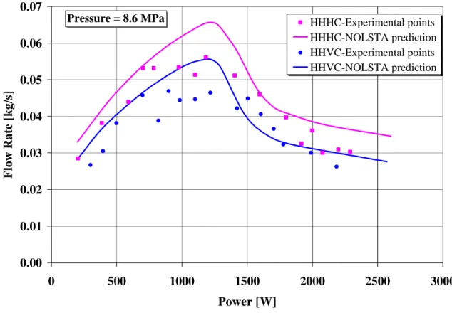
Figure 3-7. Specific enthalpy and specific heat at constant pressure for CO2 at 8.6 MPa... 31

Figure 3-8. Steady state flow rate at 8.6 MPa in HHHC and HHVC configurations ... 31

Figure 3-9. Start-up from rest at different powers (IAEA, Annual Progress Report 2010)... 32

Figure 3-10. Instability observed at 500 W, 9.1 MPa and 10.1 lpm secondary flow ... 33

Figure 3-11. Detail of heater outlet temperature oscillations at 500 W ... 33

Figure 3-12. Instability observed at 800 W, 9.1 MPa and 15 lpm secondary flow ... 33

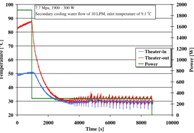
Figure 3-13. Temperature oscillations due to large power decrease (1900 – 300 W) at 7.7 MPa ... 34

Figure 3-14. Detail of temperature oscillations at 300 W due to large power decrease (1900 – 300 W), at 7.7 MPa ... 34

Figure 3-15. Pressure drops across the heater due to large power decrease (1900 – 300 W), at 7.7 MPa ... 34

Figure 3-16. Horizontal/ vertical heater test section for H2O ... 35

Figure 3-17. Schematic of the SPNCL for H2O... 36

Figure 3-18. Steady state flow rate data with supercritical water ... 37

Figure 3-19. Steady state heater inlet and outlet temperature with supercritical water ... 38

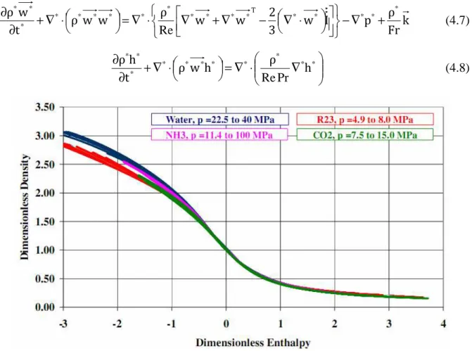
Figure 4-1. Dimensionless equation of state for H20, CO2, NH3 and R23 at different pressures... 42

Figure 4-2. Prandtl number as function of dimensionless enthalpy... 43

Figure 4-3. Thermal diffusivity as function of dimensionless enthalpy ... 43

Figure 4-4. Kinematic viscosity as function of dimensionless enthalpy... 44

Figure 4-5. RELAP5 modular structures ... 44

Figure 4-6. Schematic of difference equation nodalization ... 47

Figure 4-7. Nodalization of the BARC facility (HHHC case) adopted for RELAP5/Mod 3.3 52 Figure 4-8. Picture of vectors in diffusive term calculation ... 57

Figure 4-12. STAR-CCM+ frontal view of the bottom left bend of the loop ... 59

Figure 4-13. Detail of piece-wise linear interpolation of cp around the pseudocritical temperature (311.05 K)... 60

Figure 4-14. CO2 properties: cp, ρ, k, µ as function of temperature at 8.6 MPa ... 61

Figure 4-15. Detail of cubic splines interpolation of cp around the pseudocritical temperature (311.05 K)... 62

Figure 4-16. Schematic of boundary conditions applied to the BARC loop (colours obtained by temperature contour)... 63

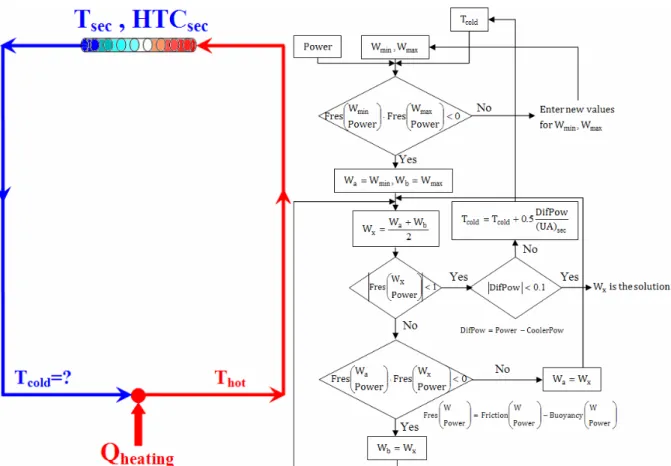
Figure 4-17. Loop with punctual sources and flowchart of the numerical scheme adopted .... 66

Figure 4-18. Loop with punctual heater and real cooler, and flowchart of the numerical scheme adopted... 67

Figure 4-19. Picture of the cooler discretized... 67

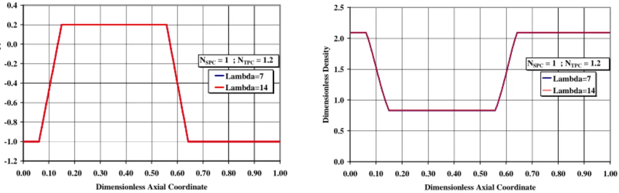
Figure 4-20. Dimensionless code nodalization of the BARC facility ... 70

Figure 4-21. Heating-cooling and gravity distribution factors ... 70

Figure 4-22. Dimensionless enthalpy and density distribution along the loop ... 71

Figure 4-23. Example of zR contour plot... 72

Figure 5-1. Schematic of the open loop condition with imposed cooling flux ... 75

Figure 5-2. Steady-state SC water (P=25 MPa) flow rate with smooth tube and rough tube .. 76

Figure 5-3. Supercritical water heater outlet temperature as function of the heating power ... 77

Figure 5-4. Steady-state flow rate at 25 MPa and 30 MPa... 77

Figure 5-5. Steady-state flow rate with different heater inlet temperature... 78

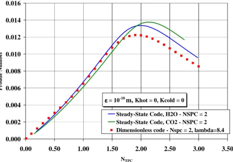
Figure 5-6. Steady-state code dimensionless code results ones with H20, CO2, NH3 and R23 79 Figure 5-7. Plot Fr-NTPC for H20, CO2, NH3 and R23 with NSPC = 0.52 ... 81

Figure 5-8. Position of water, ammonia, carbon dioxide and R23 in the plane ZC-ω... 81

Figure 5-9. Fr-NTPC characteristics for different NSPC... 82

Figure 5-10. Fr-h*hot characteristics for different NSPC... 83

Figure 5-11. Mass flow rate vs. NTPC for CO2 and different NSPC... 83

Figure 5-14. Comparison of Fr-NTPC characteristics obtained by in-house codes increasing

NSPC... 85

Figure 5-15. Comparison of Fr-NTPC characteristics obtained by in-house codes with a rough tube... 86

Figure 5-16. Agreement of in-house codes in the subcooling region ... 86

Figure 5-17. Flow rate predicted by Fluent and STAR-CCM+ codes ... 88

Figure 5-18. Heater inlet and outlet temperature at different powers as calculated by Fluent 89 Figure 5-19. Plot of heating and cooling powers versus heater inlet temperature calculated by Fluent ... 89

Figure 5-20. Temperature and density contour plots of the SC CO2 in the loop at 1400 W as calculated by Fluent ... 90

Figure 5-21. Detail of CO2 temperature in the heater section at 1400 W ... 91

Figure 5-22. Detail of CO2 temperature in the cooler section at 1400 W... 91

Figure 5-23. Temperature and velocity magnitude of the left bottom bend for CO2 at 1400 W ... 91

Figure 5-24. Temperatures at the cooler outlet and heater inlet thermocouples sections for CO2 at 1400 W ... 92

Figure 5-25. Temperature and density at the heater outlet thermocouples section (T15 – T16) for CO2 at 1400 W ... 92

Figure 5-26. Effective viscosity and thermal conductivity at the heater outlet thermocouples section at 1400 W... 93

Figure 5-27. Turbulent kinetic energy and turbulent dissipation rate at the heater outlet thermocouples section at 1400 W ... 93

Figure 5-28. Flow rate versus power with different secondary HTC ... 94

Figure 5-29. Flow rate versus power with different secondary coolant temperature ... 95

Figure 5-30. Flow rate versus power with different environmental HTC ... 96

Figure 5-31. Flow rate versus power with different values for tube roughness... 96

Figure 5-32. Flow rate versus power at different pressure ... 96

Figure 5-33. Prediction of flow rate by the CFD codes ... 98

Figure 5-36. Heater inlet and outlet temperatures as calculated by Fluent ... 101 Figure 5-37. Heater inlet and outlet temperatures as calculated by STAR-CCM+... 101 Figure 5-38. Sensitivity of flow to the secondary heat transfer coefficient as calculated by Fluent ... 102 Figure 5-39. Sensitivity of temperature to the secondary heat transfer coefficient as calculated by Fluent ... 102 Figure 5-40. Temperature contour plot at the heater outlet as computed by Fluent at 8017 W

... 103 Figure 5-41. Temperatures in the horizontal heater outlet thermocouple section as computed by Fluent at 8017 W ... 103 Figure 5-42. Temperature contour plots respectively at the heater outlet and at 230 mm far from it at 8017 W ... 104 Figure 5-43. Temperature contour plot of a cross-section of the heater wall as computed by Fluent at 8017 W ... 104 Figure 5-44. Temperature and specific heat at the thermocouple location computed by Fluent at 7792 W ... 105 Figure 5-45. Temperature and enthalpy in the thermocouple computed by Fluent at 8017 W

... 105 Figure 5-46. Steady state flow rate for a rough tube ... 106 Figure 5-47. Steady state flow rate for a smooth tube... 106 Figure 5-48. Relap5 transient calculation at high power terminated with a failure (23 MPa)107 Figure 5-49. Relap5 transient calculation near to 8 kW of power showing the flow rate

decrease (25 MPa) ... 107 Figure 5-50. Temporal evolution of the temperatures predicted by Relap5... 108 Figure 5-51. Example of transient calculation performed with Relap5 to obtain steady state conditions ... 109 Figure 6-1. Schematic of the open loop and closed loop condition with imposed cooling flux

... 111

Figure 6-2. Stability map for the open loop case with cooling heat flux imposed (Λ = 7.7 ; K =

Figure 6-4. Temporal trend of the mass flow rate obtained by RELAP5 “without structures”

... 113

Figure 6-5. NTPC and powers trend obtained by RELAP5 “without structures”... 114

Figure 6-6. Flow rate oscillations obtained by RELAP5 at 175 kW ... 115

Figure 6-7. Temperature oscillations obtained by RELAP5 at 175 kW ... 115

Figure 6-8. Dimensional stability map obtained from the dimensionless one (Λ = 7.7 ; K = 0) compared with the stability thresholds obtained by RELAP5 ... 115

Figure 6-9. Stability map of Sharma et al. (2010a) for the open loop case ... 116

Figure 6-10. Stability map for the closed loop case with cooling heat flux imposed (Λ = 8.4 ; K = 2) ... 117

Figure 6-11. RELAP5 transient simulation “with heat structures” performed to achieve steady-state conditions ... 117

Figure 6-12. Oscillations in flow rate as computed by RELAP5 and Fluent “without structures” at 1 kW... 118

Figure 6-13. Oscillating heating and cooling powers obtained by RELAP5 at 1 kW after a perturbation (case “without structures”) ... 118

Figure 6-14. Oscillations in flow rate as computed by RELAP5 and Fluent without structures at 50 kW ... 119

Figure 6-15. Temperature oscillations obtained by Fluent at a power of 50 kW ... 119

Figure 6-16. Flow rates and powers at 1 kW in the transient calculations “with structures” 120 Figure 6-17. Flow rates and powers in the transient calculations at 50 kW “with structures” ... 120

Figure 6-18. Temperatures evolution in the transient calculations at 50 kW “with structures” ... 120

Figure 6-19. Flow rate trend at 50 kW in the transient calculations performed passing from structures with reduced density to the actual ones ... 120

Figure 6-20. Experimental start-up from rest at 700 W (IAEA, Annual Progress Report 2010) ... 121

Figure 6-23. Flow rates and powers of the start-up simulation at 750 W “with structures” .. 123 Figure 6-24. Temperatures for the start-up simulation at 750 W “with structures”... 123 Figure 6-25. Instability observed in the experiment with power decrease from 700 W to 500 W ... 124 Figure 6-26. Instability observed in the experiment with power increase from 600 W to 800 W

... 124 Figure 6-27. Flow rate in the case of power decrease from 700 to 500 W (walls with reduced density) ... 124 Figure 6-28. Flow rate in the case of power increase from 600 to 800 W (walls with reduced density) ... 125 Figure 6-29. Detail of flow rate oscillations at 600 W (walls with reduced density)... 125 Figure 6-30. Steady-state flow rate vs. power curves as computed by Fluent (walls with reduced density) corresponding to the operating conditions of the experimental tests. The markers indicate transient calculations, reporting the nature of the observed behaviour (stable or unstable) ... 126 Figure 6-31. Steady-state flow rate vs. power curve as computed by Fluent (walls with

reduced density) at different values of the HTC to the secondary side. The markers indicate transient calculations, reporting the nature of the observed behaviour (stable or unstable) . 127 Figure 6-32. Stability predictions respectively by NOLSTA (Sharma et al., 2010c) and Fluent at different powers ... 128 Figure 6-33. Heater inlet and outlet temperature computed respectively by NOLSTA and Fluent at different powers... 128 Figure 6-34. Effect of the heat structures density... 128

Table 2-1. Chatoorgoon’s loop data ... 8 Table 2-2. Lomperski’s loop data... 11 Table 2-3. Geometric data for Chatoorgoon’s and Jain and Corradini loop ... 17 Table 2-4. Data of supercritical CO2 natural circulation loop... 19

Table 3-1. Thermocouples measured data... 30 Table 3-2. Features of the oscillations observed (Sharma et al., 2010b)... 32 Table 3-3. Parameters of the experiments ... 37 Table 4-1. Pressures used for the calculation of SC fluids properties ... 43

Table 4-2. RELAP5 Nodalization data of the BARC facility (CO2 SPNCL) ... 50

Table 4-3. Fluent mesh details... 58 Table 4-4. Thermal properties of AISI 347 material (Incropera, 1996) ... 62 Table 5-1. Data on the condition of max flow rate... 76 Table 5-2. Operating conditions for the simulations with different SC fluids ... 79 Table 5-3. Critical Compressibility Factors and Pitzer Acentric Factors extracted by Reid et al. (1987)... 81 Table 5-4. Results in the point of maximum Froude number... 82 Table 5-5. Variability of Λ by increasing NSPC with ε = 10-10 m... 85

Table 5-6. Variability of Λ by increasing NSPC with ε = 5·10-5 m... 85

Table 5-7. Experimental and simulation CO2 data ... 87

Table 5-8. Summary of CO2 Fluent results ... 90

Table 5-9. Values used in the sensitivity analysis ... 94 Table 5-10. Effect of different values of HTCenv at similar power conditions... 95 Table 5-11. Experimental and simulation H2O data... 97

Table 5-12. Summary of H2O Fluent results ... 100

Roman Letters

A area [m2] Λ friction dimensionless group [-]

cp specific heat at constant pressure [J/(kgK)] µ dynamic viscosity [kg/(ms)]

D diameter [m] ν kinematic viscosity [m2/s]

Dh hydraulic diameter [m] ρ density [kg/m3]

f friction factor [-]

fg gravity distribution function [-] Subscripts

fq heat flux distribution function [-] c critical

Fr Froude number [-] in inlet

g gravitational acceleration [m/s2] out outlet

G mass flux [kg/(m2s)] PC pseudocritical

h specific enthalpy [J/kg] r reduced conditions

H height [m] t turbulence

k thermal conductivity [W/(mK)] w wall

k turbulent kinetic energy [m2/s2]

K singular pressure-drop coefficient [-] Superscripts

L length [m2] * indicates dimensionless values

Npch phase change number [-]

Nsub subcooling number [-] Abbreviations

NSPC sub-pseudocritical number [-] CFD Computational Fluid Dynamics

NTPC trans-pseudocritical number [-] HTC Heat Transfer Coeff. [W/(m2K)]

p pressure [Pa] NC Natural Circulation

Pr Prandtl number [-] RANS Reynolds-Averaged Navier-Stokes

q” heat flux [W/m2] SC Supercritical

q”’ volumetric heat source [W/m3] SCWR Supercritical-Water-cooled Reactor

Q power [W] env Environment

Re Reynolds number [-] sec Secondary

t time [s]

T temperature [K]

v specific volume [m3/kg]

V volume [m3]

w velocity [m/s]

W mass flow rate [kg/s]

Greek Letters

α

β isobaric thermal expansion coefficient [K-1]

δ Dirac delta function [m-1]

General background

During the nuclear era, many several power plant concepts were proposed and built; these concepts were different mainly for the choice of moderator, coolant and layout. However, nowadays the Light Water Reactors (LWRs) have become the industrial standard in the sector, with a share close to 90% of all operating nuclear power plants (Tulkki, 2006). Though the LWRs are by far more widespread than the heavy water and gas cooled reactors, they also seem to have reached their physical limitations in terms of efficiency, cost reduction and passive safety. For these reasons, the next generation of nuclear energy systems, known as Generation IV, requires further improvements in terms of efficiency, cost, safety and reliability with respect to the current Generation III (GIF, 2002).

Six reactor projects are included in Generation IV, being the Fast Reactors cooled by gas (GFR), by Lead (LFR) and by Sodium (SFR), the Molten Salt Reactor (MSR), the Very-High-Temperature Reactor (VHTR) and the Supercritical Water Reactor (SCWR). Recently, in the frame of the European Union, priority was given to the concept of sodium fast reactor, on which design, construction and operation experience already exists, with alternative options being the lead cooled fast reactor and the gas fast reactor. Nevertheless, the supercritical water reactor has been the subject of a huge European and worldwide effort (see e.g., the HPLWR2 Project Web Site), in which several design problems were tackled and solutions were proposed; this concept is therefore still playing an important role in the Generation IV worldwide panorama because of its promising characteristics.

The SCWR concept envisages that the cooling and moderation of the core (for the thermal neutron spectrum option) is accomplished by light water at pressures higher than the critical one (hence the adjective “supercritical”). The use of light water at supercritical pressures (25 MPa) avoids boiling (no phase change between liquid and gas), and therefore the temperature can be raised considerably (up to 550 °C) as there is no risk of a thermal crisis, in favour of higher efficiencies, evaluated to be up to 45% (Duffey et al., 2010). Though it is basically a single-phase fluid, the large enthalpy change possible in supercritical water reduces the coolant flow rate as well as the pumping power, while the adoption of a direct cycle simplifies the nuclear system, eliminating the need of recirculation lines, pressurizer, heat exchanger, steam separators and dryers (Schulenberg and Starflinger, 2010). In summary, the SCWR design takes advantage of the very desirable feature of the Boiling Water Reactors (BWRs) with respect to the Pressurized Water Reactors (PWRs), being the

direct cycle, without the associated disadvantage of dealing with a two-phase flow system in normal operation, with all the associated complications.

Nevertheless, though there are large benefits from the employment of SCWRs, the design difficulties and technological challenges, mainly in terms of material resistance, together with the need to get reliable models for the physical phenomena occurring with supercritical fluids, require a significant effort in terms of research and development. Indeed, in supercritical water reactor operating conditions, the thermodynamic and transport properties of water change remarkably as the temperature approaches the “pseudocritical point”, corresponding to a sharp maximum observed in specific heat.

As an example, the large changes in density, similar in magnitude to those encountered during boiling, make the SCWR core susceptible to flow instabilities similar to those observed in BWRs (such as density-wave instabilities and coupled neutronic thermo-hydraulic instabilities). Since the operation with unstable flow is highly undesirable, as it can lead to power oscillations, causing mechanical vibration of components and challenging the control system, the deployment of SCWRs is conditioned to the design of stable systems.

In this aim, it is necessary to clearly understand and predict the instability phenomena occurring with supercritical fluids and to identify the variables which affect these phenomena.

Motivation for the present work

Natural circulation is known to be a relevant phenomenon for nuclear reactors since it involves several regimes of reactor operation. Though the natural circulation phenomena at subcritical pressure, both in single and two-phase flows, have been thoroughly studied, the same cannot be said for natural circulation with supercritical fluids. Indeed, very few experimental studies on natural circulation with supercritical fluids are reported in previous literature (see e.g., Zuber, 1966, and Lomperski et al., 2004).

The University of Pisa and the Bhabha Atomic Energy Centre (BARC) of Mumbai, India, are both involved in the Coordinated Research Project (CRP) of the International Atomic Energy Agency (IAEA) on “Heat Transfer Behaviour and Thermo-hydraulics Codes Testing for SCWRs”. This IAEA CRP promotes international collaboration among IAEA Member States (Usa, Russia, China, UK, Canada, India, Italy and other Countries) with the aim to collect accurate data on heat transfer, pressure drops, natural convection and stability regarding fluids at supercritical pressure as well as to develop reliable thermal-hydraulic codes for SCWRs.

In the frame work of this co-operation, the experimental data obtained at the BARC, related to natural circulation with CO2 and H2O at supercritical pressures, were used in this

work to test the predictions of different system and CFD codes: RELAP5/MOD3.3 (SCIENTECH Inc., 1999), Fluent (Fluent Inc., 2006), STAR-CCM+ (CD-Adapco, 2009) as well as specifically developed in-house codes.

The study, performed in cooperation with BARC, addressed most of the experimental information made kindly available in its researches, involving steady-state analyses for carbon

dioxide and water, as well as transient analyses (only for CO2); the actual operating conditions

of the experiments, as well as various others like “open loop” and “closed loop” configurations with imposed cooling flux, were considered in order to provide an overview of the capabilities of available computational tools in predicting natural circulation phenomena.

Thesis outline

The work is subdivided into seven chapters which are organized in two parts.

The first part is devoted to present a short literature review on natural circulation with supercritical fluids and to describe the reference experimental data obtained at BARC and the methodology of analysis adopted in the work. The second part, instead, describes the code results for steady-state conditions as well as the transient simulations run aiming to characterise the free evolution of the system.

More specifically, Chapter 2 presents the investigations, mostly of numerical nature, carried out on natural circulation with supercritical fluids in past studies. Chapter 3 presents the reference experimental facility, the Supercritical Pressure Natural Circulation Loop (SPNCL) of BARC, and the steady-state and stability data obtained with carbon dioxide and water at supercritical pressures; tests characterizing the loop in terms of friction factor, localised pressure loss coefficients and heat losses are also described, as well as the operating procedure adopted in the experiments. Chapter 4 presents the computational tools used in the work: the RELAP5/MOD3.3 system code (SCIENTECH Inc., 1999), CFD codes as Fluent (Fluent Inc., 2006) and STAR-CCM+ (CD-Adapco, 2009), and finally, in-house dimensional and dimensionless codes. In Chapter 5, the steady-state results for the “open loop” condition with imposed cooling flux obtained by RELAP5 and the in-house codes are compared and discussed, as well as the CFD code predictions and the experimental data about the actual cooling conditions. Chapter 6 is devoted to present the results of transient analyses. Finally, Chapter 7 summarizes the main conclusions and provides recommendations for the future work.

2.

Review of investigations on natural circulation

loops with supercritical fluids

2.1

Introduction

Flow stability is usually studied by solving the time-dependent mass, momentum and energy conservation equations representing the system. These equations are generally solved either in frequency-domain or time-domain to determine stability boundaries in appropriate parameter spaces.

In the frequency-domain approach, the conservation equations along with the

necessary constitutive laws are linearized about an operating point and Laplace transformed. Stability predictions are then made by applying such well-known stability analysis methods as Bode plots, Nyquist plots, root-locus techniques, etc.. Though very valuable, results of these frequency domain approaches are valid only for infinitesimal perturbations; besides, the linear stability analysis only predicts the threshold of instability but cannot predict the limit cycle oscillations.

In the time-domain approach, the conservation equations are solved numerically

using, for example, finite-difference techniques. Usually, this approach is very time consuming when used for stability analyses, since the allowable time step size may be very small, and large numbers of cases must be run to generate a stability map. However, with ever increasing computational resources, time domain stability analysis is becoming more widespread. It is usually performed to predict the threshold value of a system parameter (for example, heat flux or power level) below (or above) which the system is stable. Usually, the set of steady-state equations are solved first, then, the steady-state solution, with a perturbation, is used as the initial condition for the transient flow. The perturbation can either be a fractional change in the steady-state solution or a small change in one or more system parameters (like heat flux, pressure drop coefficient, etc.) that lasts a short period of time. System stability can also be investigated by momentarily perturbing the boundary conditions. If the disturbance grows in time and yields sustained or diverging flow oscillations, then the steady-state system is considered to be unstable. On the other hand, if the disturbance leads to decaying oscillations resulting in convergence of flow and other field variables to the steady-state solution, then the corresponding steady-steady-state solution is considered to be stable.

2.2

Previous works

This section summarizes, in chronological order, some of the most significant papers about supercritical natural circulation loops.

Walker, B.J., Harden, D.G. – “The “density effect” model: prediction and verification of the flow oscillation threshold in a natural-circulation loop operating near the critical point”. ASME Paper No. 64-WA/HT-23, 1964 In this paper are presented the results of a theoretical and experimental investigation of the “density-effect” model, formulated by Bouré (1965), applied to a natural circulation loop operating with Freon-114 at supercritical pressure to predict the pressure and flow oscillation threshold.

Two main idealizations were made in defining the model. The first, shown in Figure 2-1(a), was the idealization of the loop geometry, which was divided into three sections:

upstream adiabatic, L0, heater section, LC, and downstream adiabatic, L1. The cooler was not

included as long as conditions entering the upstream adiabatic section and leaving downstream were specified. A constant volumetric heat flux, W, is added to the fluid in the heater section.

The second idealization, given in Figure 2-1(b), consisted in the equation of state used. The non linear-change of density with enthalpy was postulated as being the driving mechanism for the oscillations and was the only mechanism introduced into the model. This model is called “density effect” model, and was introduced analytically by Bouré (1965).

Figure 2-1. (a) Idealized schematic of the natural circulation loop. (b) Model equation of state: density-enthalpy

By making the conservation equations dimensionless (herein, small letters are used for dimensionless quantities, capital letters for dimensional ones) by means of characteristic

values, handling, linearizing and applying the method of small perturbations, Walker and Harden, assumed the expression for the entrance velocity as:

ct 0 0 t u v e

u ( )= _∞ + (2.1)

where v0 is small in comparison with u∞, the steady state velocity, and c is a complex number

taken as

c=r+iω (2.2)

The “equation in c” investigated for the case of a pure oscillatory solution (r = 0), led to a

hypersurface (Σ) function of u∞ , a dimensionless entrance velocity, g, a dimensionless gravity

parameter and s, a dimensionless subcooling, defined as:

) , , ( ) (Σ =Σ u_∞ g s ; ( ) ; C 0 C 2 2 0 C C 0 C H H s L W R H G g WL R H U u_∞ = ∞ = = (2.3)

Figure 2-2. Comparison of theoretical and experimental results with Freon-114 at 3.62 MPa (Pcr = 3.25 MPa) The experimental instability points, as shown in Figure 2-2, revealed for supercritical pressures a good agreement with the threshold surface given by equation (2.3) by plotting

u∞= u∞(g) with s as a parameter. The operating range of temperature of the performed runs is

not reported in the paper.

Chatoorgoon, V. – “Stability of supercritical fluid flow in a single-channel natural-convection loop” International Journal of Heat and Mass Transfer 44 (2001) 1963-1972

In this paper, Chatoorgoon investigated a natural circulation loop with supercritical water (see Table 2-1) and the boundary condition of imposed heating and cooling heat flux. He performed a stability analysis, developed a stability theoretical criterion and also compared the results of the SPORTS with analytical ones.

Figure 2-3 NC loop studied Pin 25 MPa Tin 350 °C Boundary condition Pout 25 MPa Area 0.0044 m2 ID 0.0785 m Hloop 14 m Width 6 m z1 3 m z2 20 m z3 17 m f1 0.167 f2 0.0567 f3 0.0381

f includes also the local loss coefficient

Table 2-1. Chatoorgoon’s loop data

The SPORTS code is a non-linear code originally developed to investigate the stability of flows at low pressure due to subcooled boiling; it detects flow instability by introducing a perturbation in the inlet flow rate and executing a time transient. The loop investigated is shown in Figure 2-3; it has uniform cross section area and a distributed heat source and sink applied respectively along the lower horizontal leg AB and the upper horizontal leg CD.

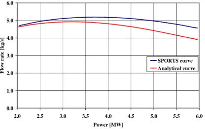
The most significant result emerged from steady state analysis with the code was the non-monotonic evolution of the flow vs. power characteristic and its good agreement with the mass flux obtained by analytical means (Figure 2-4).

0.0 1.0 2.0 3.0 4.0 5.0 6.0 2.0 2.5 3.0 3.5 4.0 4.5 5.0 5.5 6.0 Power [MW] F lo w r a te [ k g /s ] SPORTS curve Analytical curve

Figure 2-4. Flow-power curves obtained with SPORTS code and analytically

For the sake of simplicity, to develop the analytical solution, the heat source and sink were not considered uniformly distributed along a finite length, but were assumed to be point source and sink located in the middle of the segments AB and CD, thus partitioning the loop

problem of the spatial integration of the density terms (of the momentum equation) in the analytical derivation:

(

)

(

)

(

) (

)

{

}

The expression of the mass flux shows how the heating power, affecting the hot leg density

ρ2, influences also the mass flux by means of the buoyancy term at the numerator (ρ1 − ρ2)

and the friction term at the denominator (f2z2/ρ2).

Equation (2.4) helps to explain the trend of the curve flow vs. power curve, firstly increasing and then decreasing; before the maximum, the mass flow rate increases with power as the enhanced driving head is counterbalanced by friction losses at higher flow rates, while beyond the maximum, the mass flow declines with power because the rise in hot leg velocity increases enough friction losses that the balance between circulation driving head and friction losses occurs at lower mass flow rates.

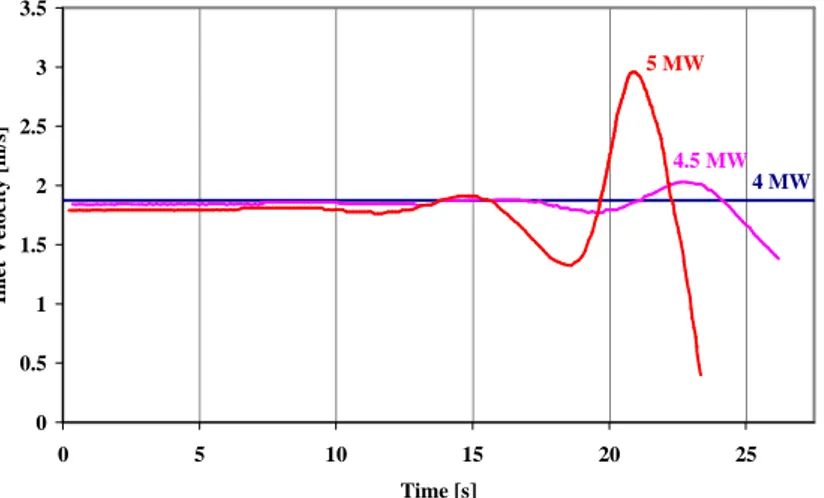
From some stability simulations carried out with the SPORTS, Figure 2-5, it turned out that flow instability occurred for powers above 4.5 MW, i.e. larger than the power corresponding to the maximum flow rate.

0 0.5 1 1.5 2 2.5 3 3.5 0 5 10 15 20 25 Time [s] In le t V el o ci ty [ m /s ] 5 MW 4.5 MW 4 MW

Figure 2-5. Stability prediction by the SPORTS code for the considered loop

Chatoorgoon suggested, therefore, that the threshold of instability could be detected by the approximate criterion: 0 ρ G 0 Q G 2 = ∂ ∂ = ∂ ∂ equally or (2.5)

(

)

(

)

This choice was derived from the study of the sign of the first derivative of G versus

ρ2: this derivative is negative in the region below the peak and positive beyond it. A

perturbation that raises the outlet fluid temperature (e.g., a decrease in flow rate) would

reduce the hot leg fluid density, and then, below the peak power where G_m =ξρ₁Φis negative

(∂G ∂Qis positive), the consequent change in flow rate would be positive, which would

counteract the perturbation. Beyond the peak power, instead, ∂G ∂ρ2 is positive, then the

change in flow rate would be negative, which would amplify the perturbation. The same reasoning applied to a negative temperature perturbation (increase of flow rate) indicates flow instability in the region beyond the peak of the flow rate versus power curve.

Solving the equation (2.5), Chatoorgoon obtained the analytical expressions for the maximum mass flow and for the corresponding thermal power;, this highlighting highlighted how that the power corresponding to the maximum flow depends only on the inlet conditions and the geometric characteristics of the loop.

Φ ξρ G_m = ₁               = 1 Φ ρ B Φ ξρ A Q 2 η 1 1 1 b - (2.7)

where the friction terms Φ and ξ are equal to

θ θ θ Φ≡ + 2 + 3 3 1 1 2 2 z f z f z f θ + ≡ 2 2 2 z f gDh 2 ξ ≡ (2.8)

In addition, B and η2 in equation (2.7) are constants, derived from an approximate water

equation of state in the addressed range:

2 2 2 η h B ρ = ; B=1.7418⋅1023 η₂ =3.277 (2.9)

Lomperski, S., Cho, D., Jain, R., Corradini, M. L. – “Stability of a Natural Circulation Loop with a Fluid Heated Through the Thermodynamic Pseudo-critical Point” - ICAPP'04: 2004 international congress on advances in nuclear power plants, Pittsburgh, PA (United States), 13-17 Jun 2004

This is one of the first published works of an experiment of supercritical fluid in a natural circulation loop and, therefore, it is particularly important and relevant. Before this work, only Harden and Boggs (1964) and Cornelius and Parker (1965) investigated experimentally the transient behaviour near the pseudocritical point of a closed natural circulation loop with Freon-114 as working fluid.

Lomperski et al. (2004) conducted experiments with supercritical CO2 in a

natural-circulation loop. CO2 was used in lieu of water to permit operation at more moderate

temperature and pressure, and also because carbon dioxide is considered a good substitute for water, as it has analogous change in physical properties across the pseudocritical point.

Even though the focus of Lomperski’s work was to investigate experimentally the

stability of closed-loop natural circulation for the CO2 bulk fluid temperature passing through

the pseudocritical point, the paper also includes results from a numerical model developed to predict flow stability.

The implemented test apparatus was a rectangular loop consisting of horizontally-oriented heating and cooling sections joined by two vertical pipes high 2 meters (see Figure 2-6). The main data of Lomperski’s loop are summarized in Table 2-2.

A measurement of differential pressure across the heat exchanger was used to monitor signs of flow instability while the steady-state flow rate was determined by an energy balance that utilized the measured electrical power input and the fluid enthalpy change between the heater inlet and outlet.

Table 2-2. Lomperski’s loop data

Pipe material AISI 316 stainless steel Heater section 1 meter long, AC current

Max heater power 15 kW

ID: heater, risers and elbows 14 mm

Risers height 2 m

Type Two tube in tube heat exchanger in parallel

ID 9.4 mm

Cooler section: heat exchanger

Length 6 m per heat exchanger Secondary coolant Water/glycol mixture

Cover gas Helium

Pressurizer

Free volume 1.7 liters

Thermocouples K-type,

7 fluid thermocouples, 15 wall thermocouples

System pressure 80 bar

(a) (b)

Figure 2-6. (a) Schematic of NC Lomperski’s loop. (b) Operating curve for SCCO2 test loop

The tests run consisted of stepwise increases in input power followed by a waiting period to allow the system to stabilize at a new flow rate. The secondary side conditions were occasionally adjusted to maintain the target cold leg temperature of 24 °C and gas was bled from the pressurizer to keep the system pressure near 80 bar.

The experiments (see Figure 2-7) were conducted in two different configurations: a base case without flow obstructions in order to maximize the flow rate, and a second one with a 6 mm-diameter orifice within the hot leg (the addition of flow resistance in the hot leg lowers the threshold power at which flow instabilities develop).

Over the course of testing, the loop has been operated within these ranges of conditions: inlet temperature 20-30 °C, outlet temperature 40-85 °C; pressure 75-95 bar. No flow instabilities have been observed despite attempts to produce them with perturbations to the power input: the system is always returned to steady state after such perturbations, as shown in Figure 2-8.

Figure 2-8. Power perturbations with Tinlet ~23°C

Lomperski et al. developed also a computer code to study stability behaviour. Numerical simulations were carried out using initial conditions corresponding to both the positive and negative slope regions of the steady state mass flow versus power; the results obtained were that positive slope region identifies a stable area, while the negative slope region an unstable one, in which the calculated flow rate always diverged after a short time.

The only difference between the model and the experimental apparatus was the absence of the pressurizer in the numerical simulations, but experimental tests done on it suggested that the pressurizer is not the source of unexpected loop stability.

Lomperski et al., because of the absence of oscillations in experiments, suggested that the instabilities observed with the code could be numerical in nature.

Prashant K. Jain, Rizwan-uddin – “Numerical analysis of supercritical flow instabilities in a natural circulation loop” Nuclear Engineering and Design 238 (2008) 1947–1957

In this work, Jain and Rizwan-uddin investigated flow instabilities in a natural circulation

loop with supercritical CO2 through a computer code written in FORTRAN 90.

The main contribution of this paper was in the study of the effects of numerical discretization parameters on stability threshold. Stability results, in fact, can change refining

spatial and temporal grid until results’ independence is reached with respect to the adopted grid (convergence analysis).

A schematic diagram and geometric parameters for the investigated loop are shown in Figure 2-9. It is a constant area loop with lower horizontal heating and upper horizontal cooling sections. Heat source and sink were assumed to be of equal magnitude, and uniformly distributed along the respective sections. Energy was assumed to be directly deposited to or extracted from the respective sections eliminating the need to model wall heat transfer mechanism. Both, inlet and outlet of the loop were assumed to be connected to a large reservoir or pressurizer chamber in order to maintain constant inlet conditions (i.e. constant pressure and temperature at point A).

Figure 2-9. Schematic diagram of Jain and Rizwan-uddin loop

As shown in Figure 2-10, with a temporal grid refinement study, Jain and Rizwan-uddin have shown that a level power of 1 MW, well below the stability threshold of 1.51 MW found with

∆t = 0.35 s, can be revealed as unstable further reducing the time step.

This meant that a ∆t = 0.35 s (adopted in previous work by Chatoorgoon et al., 2005b) was a time step too large for an accurate stability analysis; in fact, it is well known that a large time step may induce numerical diffusion and hence artificial flow stability into the system. In Figure 2-11 is shown how a not enough small time step could lead to a strongly wrong stability prediction.

Further reductions of the time step yielded a time step size independent converged solution at t = 0.021875 (0.35/16) s.

Figure 2-10. Effect of reducing time step on the transient solution at 1.0 MW

Figure 2-11. Comparison of stability prediction with previous investigations

Differently, the spatial grid refinement study has revealed that reducing the spatial grid size does not have a meaningful effect on system stability, as the system remained stable at finer spatial resolutions producing spatially converged results.

Jain and Rizwan-uddin investigated also that the stability behaviour for different inlet subcooling founding, as shown in Figure 2-12, a similar behaviour to that observed in two-phase heated channel systems (Boure et al., 1973).

Figure 2-12. Effect of inlet subcooling on threshold power

From the results presented in this paper, Jain and Rizwan-uddin concluded that the stability threshold of a natural circulation loop with supercritical fluid is not confined to the near-peak region of the steady state flow-power curve, as reported previously by Chatoorgoon et al. (2005b).

Manish Sharma, D.S. Pilkhwal, P.K. Vijayan, D. Saha, R.K. Sinha – “Steady state and linear stability analysis of a supercritical water natural circulation loop” Nuclear Engineering and Design 240 (2010) 588–597 In this work, Sharma et al. (2010) carried out a linear stability analysis of a supercritical water natural circulation loop through the code SUCLIN. The boundary condition used was of cooling heat flux imposed, that even if it is something that is not very much close to the physics of a real loop, it was consistent with the previous works of Chatoorgoon et al. (2005a) and Jain and Corradini (2006). Through the study of stability maps generated by the linear code SUCLIN, Sharma et al. focused on the effects of diameter, loop height and local loss on stability behaviour. The stability maps set up for different loop geometries, for instance, highlighted a very different threshold of instability for Chatoorgoon loop and Jain and Corradini loop.

As shown in Figure 2-13, beyond a heater inlet temperature of 365 °C, from the stability map of Chatoorgoon’s loop resulted that the system should be stable whatever power is added, while the same effect was obtained with an inlet temperature of 220 °C for Jain and Corradini loop. The reason of this remarkable difference could be identified by the different geometric values of the loops reported in Table 2-3, and especially by H/ID, ratio between height and inner diameter of the loop.

Figure 2-13. Stability maps for Chatoorgoon’s loop and Jain and Corradini loop, both at 25 MPa, predicted by SUCLIN code.

Table 2-3. Geometric data for Chatoorgoon’s and Jain and Corradini loop

ID 78.5 mm ID 42.9 mm

Hloop 14 m Hloop 3 m

Width 6 m Width 2 m

Chatoorgoon’s loop

H/ID 178.3

Jain and Corradini loop

H/ID 69.9

The single effects of the internal diameter and of loop’s height on stability, are shown in the stability maps of Figure 2-14, generated for another supercritical water loop corresponding to a supercritical test facility set up in BARC (Bhabha Atomic Research Centre).

By increasing the diameter the power envelope of the unstable zone increases notably, while the heater inlet temperature beyond which instability is not observed decreases.

The same behaviour occurs by raising loop height.

The effect of local losses on the stability behaviour is shown in Figure 2-15. As in two-phase natural circulation loops, local losses in cold or sub-critical leg stabilizes, while local losses in hot or supercritical leg destabilizes.

Figure 2-15. Effect of local losses on stability behaviour

Manish Sharma, P.K. Vijayan, D.S. Pilkhwal, D. Saha – “Experimental and theoretical investigations on the steady state and stability behaviour of Natural Circulation Systems operating with supercritical fluid”. IAEA Technical Meeting on Heat transfer, thermal-hydraulics and system design for supercritical pressure water cooled reactors, 5-8 July 2010 Pisa, Italy

In this work, the experimental results obtained in a closed natural circulation loop (SCNCL) with supercritical carbon dioxide were compared with those of the computer code NOLSTA. Sharma et al. carried out a steady state and stability analysis of open and closed loop.

In the open loop analysis, the inlet fluid temperature to heater is fixed irrespective of the heater power, the rate of heat rejection in the cooler is not evaluated based on calculation of overall heat transfer coefficient for cooler and temperature difference between primary and secondary fluid. Whatever the amount of heat generated in the heater, it is rejected in the cooler without evaluating its capacity of heat removal. In this case, the operating pressure of the loop, inlet fluid temperature to the heater and the heater power are specified.

In the closed loop analysis, the coolant mass flow rate on secondary side of cooler is kept constant as heater power is increased, the heater inlet temperature is not fixed and increases with increase in heater power. The rate of heat rejection in the cooler is evaluated based on calculation of overall heat transfer coefficient for cooler and temperature difference

between primary and secondary fluid. In this case, the operating pressure of the loop, coolant mass flow rate & inlet temperature for secondary side of cooler and the heater power are specified.

The schematic of the test facility is shown in Figure 2-16, while geometric data of the loop are listed in Table 2-4.

Figure 2-16. Schematic of Sharma ‘s natural circulation loop Table 2-4. Data of supercritical CO2 natural circulation loop

Pipe material AISI 347 stainless steel Heater section 1.3 meter long, AC current

OD / ID 21.34 mm / 13.88 mm

Height 4.1 m

Width 3.01 m

Type Tube in tube heat exchanger

Length 1.2 m

Cooler:

OD / ID 88.9 mm / 77.9 mm Secondary coolant Chilled water (9 °C) Secondary volumetric flow rate 10 – 56 LPM

Pressurizer: cover gas Helium

Possible configuration HHHC; HHVC; VHHC; VHVC Operating pressure 8 - 9 MPa

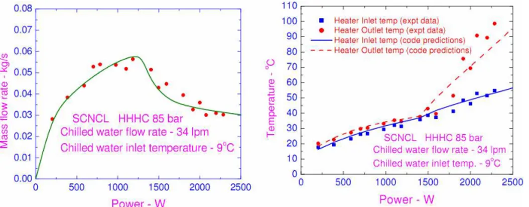
In the closed loop analysis, the steady mass flow rate obtained from the code NOLSTA showed a good agreement with the experimental results (Figure 2-17).

It can be observed that the heater inlet temperature is no more constant, as in open loop analysis, and that the major difference of flow-power curves respect of previous investigations with open loop condition is the sharp reduction of flow, which occurs when the cold leg passes the pseudocritical point. (37.4 °C at 85 bar).

Figure 2-17. Comparison of experimental and predicted mass flow rate, heater inlet and outlet temperature

From experiments on instability, see Figure 2-18, resulted that the only possibly unstable configuration was the HHHC orientation (Horizontal Heater Horizontal Cooler), and that the

unstable power range was 500÷925 W. A typical characteristic of this instability shown by

experiments, was that only heater outlet temperature oscillated while the heater inlet temperature remained practically constant indicating a open loop type behaviour.

Figure 2-18. Experimental unstable behaviour observed at 700 W and 800 W for HHHC orientation

The stability analysis carried out for HHHC orientation with the code NOLSTA (Figure 2-19) showed remarkable differences with the experimental results: the loop was found to be

unstable in a larger power range, 800÷1400 W, flow reversal was predicted and inlet heater

3.

Reference experimental data

In this chapter the experimental facility of the BARC (Bhabha Atomic Research Centre,

Mumbai, India) used to perform experiments on supercritical CO2 natural circulation is

described. The experiments carried out are also reported.

3.1

Experimental facility

In Figure 3-1 it can be seen the schematic of the experimental loop. It is a uniform diameter rectangular loop made of 13.88 mm inside diameter stainless steel (SS-347) pipe, with an outside diameter of 21.34 mm. The loop has two heater test sections and two cooler test sections, so that it can be operated in any one of the four orientations such as Horizontal Heater Horizontal Cooler (HHHC), Horizontal Heater Vertical Cooler (HHVC), Vertical Heater Horizontal Cooler (VHHC) and Vertical Heater Vertical Cooler (VHVC).

The heater was made by uniformly winding nichrome wire over a layer of fiber glass insulation. The cooler was of the tube-in-tube type with chilled water as the secondary coolant flowing in the annulus. The outer tube, forming the annulus, had a 77.9 mm inside diameter and 88.9 mm outside diameter. The loop had a pressurizer connected to the bottom horizontal pipe which takes care of the thermal expansion besides accommodating the cover gas helium above the carbon dioxide. The safety devices of the loop (i.e. rupture discs RD-1 & RD-2)

were installed on top of the pressurizer which also had provision for CO2 & He filling.

The entire loop was insulated with three inches of ceramic mat (k=0.06 W/(mK) ).

3.1.1 Instrumentation

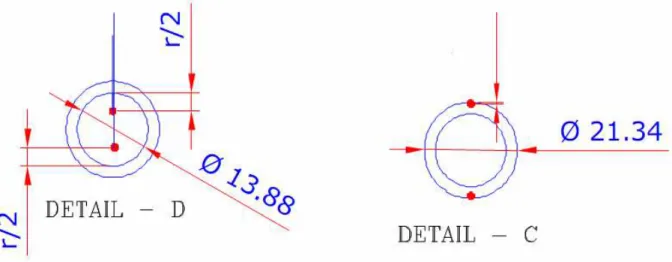
The BARC loop was instrumented with 44 calibrated K-type mineral insulated thermocouples (1 mm diameter) to measure the primary fluid, secondary fluid and heater outside wall temperatures. Primary fluid temperatures at each location were measured as the average value indicated by two thermocouples inserted diametrically opposite at a distance of r/2 from the inside wall (see detail-D in Figure 3-3). On the other hand, secondary fluid temperatures were measured by a single thermocouple located at the tube centre. This was adequate to obtain the average temperature as the temperature rise in the secondary fluid was small (< 4 °C). The thermocouples used to measure the heater outside wall temperature (see Figure 3-2) were installed flush with the outside surface for a total of 12 thermocouples installed at six axial distances at diametrically opposite locations (see detail-C in Figure 3-3).

Figure 3-1. Schematic of the supercritical pressure natural circulation loop (SPNCL) of the BARC

The system pressure was measured with the help of two Kellar made pressure transducers located on the pressurizer as well as at the heater outlet. The pressure drops across the bottom horizontal tube and the level in the pressurizer were measured with the help of two differential pressure transmitters. The power of each heater was measured with a wattmeter, while the secondary flow rate was measured with the help of a rotameter. All instruments were connected to a data logger with a user selectable scanning rate. For all the transient and stability tests the selected scanning rate was 1 second.

The accuracy of the thermocouples was within ± 1.5 °C. The accuracy of the pressure and differential pressure measurements were respectively ± 0.3 bar and ± 0.18 mm of water column. The accuracy of the secondary flow as well as the one of power measurement are both ± 0.5 % of the reading. In addition, typical fluctuations of each instrument were also recorded during steady state with and without power (stagnant initial conditions) and a light difference was observed.

Figure 3-3. Detail of the thermocouples used to measure fluid and wall temperature

3.1.2 Characterizing loop tests

In this section, tests performed to quantify the heat losses and the pressure drops along the loop are presented. The pressure drop characterization tests were carried out under forced flow conditions with the help of a pump in a separate facility using the same bottom horizontal pipe and one of the elbows installed horizontally.

From the measured pressure drop across the bottom horizontal pipe and the flow rate, the friction factor for the pipe was estimated by the following equation:

2 m 2 m LW p Δ A ρ D 2 = f (3.1)

The estimated friction factor is plotted in Figure 3-4. together with the correlation fitted to the friction factor data. From the measured pressure drop across the elbow and the flow rate, the loss coefficient was estimated as below:

2 m m 2 W p Δ A ρ 2 K = (3.2)

The loss coefficient data generated at forced flow condition is plotted together with its fitting in Figure 3-4. The loss coefficient was found to be constant at 0.55 for Reynolds numbers greater than 45000.

Figure 3-4. Experimental friction factor and experimental K coefficient (IAEA, Annual Progress Report 2010)

To estimate the heat losses, natural circulation experiments were carried out at various powers with water at subcritical conditions. These experiments were carried out at a system pressure of 30 bar for all the four orientations of the heater and cooler.

The NC mass flow rate of subcritical water was estimated by the heat balance across the heater:

(

)

where the specific heat considered is that corresponding to the arithmetic average of heater inlet and outlet temperatures. This choice seems reasonable because, as shown in Figure 3-5, the specific heat trend is quite linear for short ranges of temperature.

The heat rejected at the cooler, Qcooler, was estimated using the measured cooler inlet and

outlet primary temperatures:

(

)

p

cooler Wc T T

Q = , − , (3.4)

In this way, it was possible estimate the heat loss fraction (Figure 3-6) as:

cooler heater Q Q Q Fraction Loss Heat = − (3.5)

4.15 4.2 4.25 4.3 4.35 4.4 4.45 4.5 4.55 100 110 120 130 140 150 Temperature [°C] C p [ k J /( k g K )] H2O : P = 3 MPa Saturation Temp. = 233.8 °C

Figure 3-5. Specific heat at constant pressure for H2O at 30 bar in the temperature range 100 – 150 °C Since the ambient temperature was significantly high (30 ± 2 °C) compared to the chilled water coolant temperature (9.8 ± 1.6 °C), in certain low power cases, heat was gained rather than lost.

However, by observing Figure 3-6 it can be noted an unusual result, i.e. the heat loss is maximum (about 20% of heater power) for HHHC orientation. Actually, it would be expected that the heat losses were maximum for the HHVC orientation since its hot leg is the longest, and minimum for VHHC orientation, since its hot leg is the shortest. Instead, what we see is that VHHC shows almost minimum heat loss as expected, whereas HHVC does not show the maximum heat loss. This discrepancy between our theoretical considerations and the heat losses calculated in this way could be due to problems of thermal stratification with HHHC orientation.

Indeed, the unavoidable thermal stratification in the horizontal heater outlet and horizontal cooler outlet leads to some error in the measured heater and cooler outlet temperatures, even if there is a mixing length available at the outlet side of both the horizontal heater and horizontal cooler. Then, the heat losses estimated could be less than that shown in Figure 3-5 for HHHC orientation. Although, it is known that there is larger error in the heat loss calculation for HHHC orientation, it was not found a better way to experimentally estimate it (a Coriolis flow meter could not be chosen because of the vibrations introduced in the system).