School of Industrial and Information Engineering
A
N EXPERIMENTAL PROCEDURE TO PERFORM MECHANICAL
CHARACTERIZATION OF SMALL
-
SIZED BONE SPECIMENS FROM
FEMORAL THIN CORTICAL WALL
Supervisor:
Prof. Pasquale Vena
Co - Supervisors:
Prof. Dario Gastaldi
Ing. Massimiliano Baleani
Master Thesis of:
Fulvio AIRAGHI Matr. 875500 -
Master of Science in Materials Engineering and NanotechnologyLivio BONANNI Matr. 875882 -
Master of Science in Biomedical EngineeringII
Ringraziamenti
Il qui presente progetto di tesi è stato reso possibile grazie alla collaborazione con il laboratorio di tecnologia medica dell’Istituto Ortopedico Rizzoli (IOR) di Bologna. Doveroso è un ringraziamento a coloro che hanno donato alla scienza il proprio corpo, permettendo alla ricerca di progredire ed avanzare; la speranza è che anche il nostro studio possa contribuire, seppur in minima parte, al progresso scientifico, valorizzando il prezioso dono da loro fattoci.
In particolare, ringraziamo l’ingegner Massimiliano Baleani e l’ingegner Roberta Fognani, il cui aiuto è stato essenziale per lo sviluppo dello studio. Non di meno, la disponibilità e l’attenzione del professor Pasquale Vena e del professor Dario Gastaldi che ci hanno guidato durante tutto il progetto di tesi.
III
Contents
Abstract VII
Sommario X
Chapter 1 - Femur: Structure, and Mechanics 1
1.1 Nano- and Micro-Structure of the Bone Tissue in the Femur 2
1.2 Mechanics 8
1.3 Toughness and Post-Yield Behaviour 11
1.4 Aim of the Study 19
Chapter 2: Materials & Methods 22
2.1 Sample preparation 22 Preliminary considerations 22 Slicing 29 Sanding 35 2.2 Experimental Procedure 39 Preliminary Considerations 39 Setup Design 42 Experimental Protocol 48
2.3 Accuracy and Repeatability 56
Accuracy tests 56
Aluminum Tests 58
Animal Tissue Tests 59
Chapter 3 – Results and Discussion 60
3.1 Results 60
Post-Rupture Analysis 66
Statistical Analysis 69
3.2 Discussion 71
V
List of Figures and Tables
Figure 1 - Visual representations of the area of interest ... VIII Figure 2 - Initial frame showcasing specimen placing ... IX
Figure 3 - Proximal femur anatomy ... 1
Figure 4 - (left) Radiograph of the proximal femur ... 4
Figure 5 - Slices from a 3D µ-CT scan of a human femur ... 5
Figure 6 - Simplified representation of the compact bone ... 6
Figure 7 - Main toughening mechanisms ... 13
Figure 8 - Visual representation of punctual and extensive damage to bone ... 14
Figure 9 - Schematization of crack progress ... 15
Figure 10 - Display of the main nano scale structures ... 16
Figure 11 - Nanoscopic 2D model of HA/collagen composite ... 17
Figure 12 - Typical stress/strain curves ... 18
Figure 13 - Three-dimensional model of a femur neck ... 25
Figure 14 - Schematic representation of the sample’s final shape ... 27
Figure 15 - Supero-lateral harvesting site ... 28
Figure 16 - Harvesting procedure ... 30
Figure 17 - Microtome setup ... 31
Figure 18 - Microtome grip ... 33
Figure 19 - Harvesting procedure ... 34
Figure 20 - Proximal half of a typical slice ... 35
Figure 21 - Pictures of a Plexiglas dish ... 36
Figure 22 - Isolation procedure ... 37
Figure 23 - Schematization of the three-point bending setup ... 40
Figure 24 - CAD model of the whole testing apparatus ... 41
Figure 25 - CAD model of the holder ... 43
Figure 26 - CAD model showcasing how the holder ... 44
VI
Figure 28 - Exploded representation of the loading wedge ... 47
Figure 29 - First and last frame of a typical bending test ... 50
Figure 30 - Typical stress/strain plot ... 52
Figure 31 - Wireframe of the nodal distribution utilized to compute surface areas ... 54
Figure 32 - Force/displacement graph for each sample, divided by donor ... 62
Figure 33 - Stress/strain graph of the obtained data ... 63
Figure 34 - Intensity scan obtained with the laser microscope from a specimen ... 66
Figure 35 - Simplified model of osteonal lamellae ... 78
Figure 36 - Two very distinct stress/strain curves produced during this study ... 79
Figure 37 - Cross section of a broken specimen ... 80
Figure 38 - Lateral view of a typical breakage site ... 81
Table 1 - Overview of the hierarchical levels of bone ... 6
Table 2 - Numerical data Young’s Moduli measured from human femur diaphyses ... 11
Table 3 - Slide accuracy data ... 57
Table 4 - Numerosity of samples for each donor subject ... 60
Table 5 - Experimental data from donor #3029 ... 64
Table 6 - Experimental data regarding donor 4771 ... 65
Table 7 - Experimental data of donor #4843 ... 65
Table 8 - Post-rupture analysis data from donor #3029... 67
Table 9 - Post-rupture analysis data regarding donor #4771 ... 68
Table 10 - Post-rupture analysis data of donor #4843 ... 68
Table 11 - Average values for each subset analysed ... 70
Table 12 - Statistical analysis made on subsets of donors ... 71
Table 13 - Compact bone’s mechanical properties find in literature ... 74
VII
Abstract
Clinical Studies show that hip fractures are generally located in either the medial or the lateral aspects of the proximal femur.
During traumatic events such as falls, the femur neck is often impacted sideways, which may lead to fractures with initiation sites in its infero-medial side, because of the unphysiological loading conditions. The elderly and the osteoporotic subjects are the ones at higher risk, since in both of these cases trabecular bone loss and cortical wall thinning occur. These conditions, in their most extreme forms, might lead to spontaneous rupture of the femur neck in its subcapital supero-lateral aspect.
It is known that bone is a highly heterogeneous tissue throughout the body, and, while plenty of research has been conducted on the femur diaphysis, few studies have addressed this subject while focusing on its proximal epiphysis.
Because of these reasons, the femur neck constitutes a region of particular interest for biomechanical investigations.
The aim of this study is to design and implement a procedure that enables harvesting and testing of small cortical bone specimens from the femoral neck. This methodology should allow to discriminate between specimens that come from different aspects of the femur neck, as well as those that come from diseased or healthy subjects.
The lateral aspect of the femur neck presents cortical tissue that is thinner (<0.5 mm) than that of the diaphysis and is curved in a double-saddle shape.
Thus, the mechanical characterization of this tissue is challenging.
An accurate sample harvesting procedure is preventively designed by simulating the cutting strategy with the aid of 3D models of the femur head from micro-CT scans.
Three human femoral necks are isolated and later sliced longitudinally 1 mm thick with a Leica SP1600 microtome. Obtained slices are subsequently sanded down in a prismatic shape with an EXAKT400CS Micro Grinding System leaving 0.4 mm of cortical bone, separated from both trabecular and periosteal tissues.
VIII
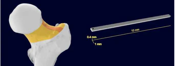
Figure 1 - Visual representations of the area of interest (left) for the harvesting procedure (orange) of the femur neck (yellow). (right) Definitive prismatic shape of extracted samples with nominal dimensions
A three-point bending setup is chosen as the best-compromise solution for the particularly small samples that can be obtained, with the purpose of identifying elastic and plastic engineering constants such as the flexural elastic modulus, yield stress and strain, ultimate stress and strain, toughness, and total dissipated energy. A uniaxial DC gear motor (M112.2DG, Physik Instrumente, DE), with a 25 mm travel range, 50 nm displacement resolution, and a maximum load of 10 N is implemented for the application of load. Force measurement is performed by means of a canister load cell (Model 31, Honeywell, US), with a measuring range of ± 5 N, and a load resolution of 1 mN. A suitably designed sample grip and a wedge are used to hold and apply the load to the sample respectively. The span between the ends of each sample is set at 8 mm, and the displacement rate of the centre is 2.5 μm/s. A monotonic bending test is carried-out on samples.
An optical stereo-microscope (Olympus SZ61) coupled with a camera (IDS GigE uEye SE), are utilized to capture images of the curvature of samples synchronized with load data. Displacement is measured with through a video tracking software (OSP Tracker app, US).
IX
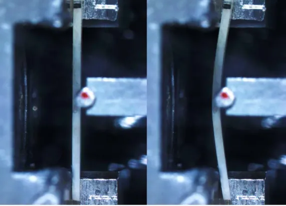
Figure 2 - Initial frame showcasing specimen placing on the test setup (left). Last frame showing curvature of the same sample before rupture (right)
A series of accuracy and repeatability tests with animal subjects (pig tibiae) and aluminum 6060 T6 specimens are made in order to validate the method. A repeatability of 2% is achieved intra-sample and 3.6% inter-sample. Accuracy falls within 1% of the true value. After assessing the accuracy and effectiveness of the aforementioned experimental procedure, a total of 41 human cortical bone samples are tested.
Measured values for Young’s Modulus are about 12.5 GPa, as well as a yield and maximum stress of 150 MPa and 200 MPa respectively.
Statistically significant differences have been found among both specimens collected from either diseased or healthy subjects, and samples collected from either the medial or lateral side of the subject’s femur neck.
These preliminary results show the effectiveness of the presented procedure in capturing intra- and inter-subject changes related to the cortical bone tissue of the femoral neck.
X
Sommario
Come emerge dagli studi presenti nella letteratura, la frattura dell’anca è solitamente figlia di un cedimento nelle regioni laterale e mediale del femore prossimale.
A seguito di cadute accidentali il collo del femore si trova ad essere sottoposto a carichi trasversali (non fisiologici) in grado di causarne la frattura, che generalmente origina dalla regione infero-mediale dello stesso. I Soggetti anziani e soggetti affetti da osteoporosi risultano essere particolarmente sensibili a questo evento traumatico poiché la qualità del tessuto osseo viene intaccata dalle suddette condizioni cliniche (perdita di tessuto trabecolare e assottigliamento del tessuto corticale). In particolare, nei casi più critici, per le suddette condizioni, può avvenire la frattura spontanea che si innesca nella zona sub-capitale dell’aspetto supero-laterale.
L’epifisi prossimale costituisce, per le motivazioni appena citate, una regione di particolare interesse per gli studi biomeccanici.
Benché sia risaputo che le proprietà strutturali e meccaniche del tessuto osseo possano presentare variazioni sia tra ossa di diversi distretti anatomici, sia tra regioni diverse dello stesso osso, solo poche ricerche sono state incentrate sulla caratterizzazione di questa a discapito di una certa numerosità di studi condotti sulla diafisi femorale.
Lo scopo di questo studio è, a tal ragione, quello di progettare e di implementare una procedura atta a estrarre e testare campioni di osso corticale del collo femorale. L’obiettivo finale è riuscire ad individuare, ove presenti, differenze nelle proprietà meccaniche fra tessuti ossei provenienti da diversi aspetti del collo femorale, e fra soggetti sani o affetti da patologie.
Dato l’esimio spessore di tessuto corticale (minore di 0.5 mm nel suo aspetto laterale) e la particolare geometria a doppia sella presenti nel collo femorale, la procedura di estrazione dei campioni risulta essere particolarmente difficoltosa. L’iter di preparazione dei provini è stato pertanto preventivamente simulato su modelli tridimensionali ottenuti da micro-Tomografie Computerizzate (μ-CT).
XI Successivamente, tre epifisi femorali sono state isolate dal resto dell’osso, e tagliate in sezioni dello spessore di 1 mm, tramite l’utilizzo di un microtomo (Leica SP1600). Le sezioni così ottenute sono state quindi levigate tramite una levigatrice (400CS Micro Grinding System), per asportare l’osso trabecolare ed il periostio dal campione finito, ed ottenere una forma prismatica il cui spessore di 0.4 mm fosse interamente composto da tessuto corticale.
Figura 1 - (sinistra) rappresentazione del collo femorale (giallo) e della zona d’interesse laterale (arancione) per la procedura d’estrazione dei campioni. (destra) Campione di forma prismatica dopo aver concluso la sua
procedura di lavorazione. Sono indicate le sue dimensioni nominali in giallo
La prova di flessione a tre punti è risultata essere la più adatta a testare i campioni ottenuti, date le loro dimensioni ridotte. Grazie a questa sono state determinate le principali costanti ingegneristiche, quali modulo elastico a flessione, sforzo e deformazione di snervamento, sforzo e deformazione massime, tenacità a frattura e l’energia totale dissipata.
Il carico della prova è stato generato tramite un attuatore lineare con una risoluzione di spostamento di 50 nm, una corsa totale di 25 mm ed una capacità massima di 10 N (M112.2DG, Physik Instrumente, DE). La misurazione delle forze applicate è stata effettuata tramite una cella di carico ad alta risoluzione (1 mN), con un intervallo di forze di ± 5 N. Al fine di allineare e sostenere il provino durante il test è stato realizzato un
XII apposito afferraggio in alluminio; analogamente un cuneo è stato ideato per sviluppare la forza applicata al centro dello stesso. I campioni sono stati testati con una prova di flessione monotona. La prova di flessione a tre punti è stata eseguita utilizzando una luce di 8 mm ed una velocità di 2.5 µm/s.
Uno stereo-microscopio ottico (Olympus SZ61) accoppiato ad una telecamera (IDS GigE uEye SE), hanno permesso di registrare una sequenza di immagini che catturano la deflessione del provino durante la prova; la frequenza di acquisizione è la stessa utilizzata per la lettura dei dati di forza, di modo che i due valori risultino essere sincronizzati fra loro. Da queste sono stati poi ricavati gli spostamenti del punto centrale della trave tramite l’utilizzo di un software di tracciamento (OSP Tracker app, US).
Figura 2 - Primo fotogramma del campione montato sul supporto per il test di flessione a tre punti (sinistra). Ultimo fotogramma prima del cedimento dello stesso, nel quale si può
apprezzare il grado di curvatura raggiunto (destra)
Prove di accuratezza e ripetibilità sono state effettuate utilizzando campioni suini (tibia) e di alluminio 6060 T6, al fine di valutare la bontà del setup sperimentale. Gli errori
XIII commessi sulla ripetibilità intra- ed inter-campione sono risultati essere minori rispettivamente 2% e del 3.6%. L’accuratezza della prova invece ha superato il 99%. Dopo aver verificato la validità e l’accuratezza di tale procedura, un totale di 41 campioni è stato testato, ottenendo un modulo elastico di circa 12.5 GPa, uno sforzo a deformazione e massimo rispettivamente intorno ai 150 e 200 MPa.
Differenze statisticamente significative sono state riscontrate tra campioni derivanti da soggetti sani e malati e tra gli aspetti mediale e laterale dello stesso soggetto.
Questi risultati preliminari mostrano l’efficacia della procedura nel catturare differenze intra- ed inter-soggetto nelle proprietà del tessuto osseo corticale del collo femorale.
1
Chapter 1 - Femur: Structure, and Mechanics
In the present study, the focus is on the femur neck. Thus, an anatomical and physiological description is presented in order to introduce to the topic.
The femur bone presents a semi-spherical head, which forms the hip joint together with the acetabulum. Distally to the head one will find the narrower cervical region, and then two massive, rough processes called the greater and lesser trochanters, situated on the superolateral and inferomedial aspects, respectively. These two are insertion points to the powerful hip muscles and are linked by the interochanteric crest in the rear end, while frontally, one can find a less pronounced line connecting them. Along the diaphysis, a groove called linea aspera is located. On its proximal side, this groove splits into pectineal
line and gluteal tuberosity, the latter of which is a crest (occasionally a depression) of the
bone where the powerful glutei maximi muscles are attached. On its distal side, the aspera line splits into the supracondylar medial and lateral lines, which keep going downward until their respective condyle.
2
The lateral and medial epicondyles are the thickest portions of the femur. These, together with the supracondylar lines are where some of the muscles of the thigh and leg, and some of the ligaments of the knee are attached.
On the distal end of the femur two smooth and rounded surfaces are found, these are the medial and lateral condyles, separated by a cleavage called intercondylar notch.
To the front of this end of the bone a smooth depression called patellar surface lies, which articulates - as the name suggests - to the patella.
In the back lies another flat surface called popliteal fossa.
The femur plays an essential role in the musculoskeletal system because the vast majority of muscular torque is applied in its proximal epiphysis during locomotion.
As such, it is one of the most investigated anatomical districts of the whole body with the aim of characterizing its mechanical properties, both in the physiological and pathological cases.
In order to have a better grasp of the problem, a brief introduction to the subject is presented in the following paragraphs.
1.1 Nano- and Micro-Structure of the Bone Tissue in the
Femur
Bone is a hard tissue comprised of a calcified load-bearing matrix, and a cell fraction that is devolved to maintaining and repairing it. Differently from typical, soft biological tissues, the cell fraction in the bone is small, and almost all the space is occupied by the matrix. The cell fraction is comprised of osteogenic cells, osteoblasts, osteocytes, and osteoclasts, while the extracellular matrix is mainly made up of hydroxyapatite crystals buried in a collagen matrix.
Osteoblasts are cells that secrete the extracellular matrix by depositing the protein phase, which later hardens through mineral deposition. High stress and fractures stimulate their
3 activation and secretion. When osteoblasts become entrapped within the extracellular matrix they differentiate into osteocytes.
Osteocytes lie in small crevices called lacunae, which are connected by a dense web of capillaries called canaliculi. Each osteocyte extends through this net and connects to other osteocytes. Osteocytes have plentiful functions: some reabsorb bone tissue, others deposit new one, both contributing to the bone renewal process as well as the homeostasis of calcium and phosphate in blood. The osteocyte web (syncytium) appears to have sensory functions as well, as these cells can detect tension and compression [29]; when the tissue is put under stress, extracellular fluid flows through the canaliculi, and this is thought to drive osteocytes to release biochemical signals that regulate bone remodelling [7].
Osteoclasts typically reside in pits called Howship lacunae, and their destructive behaviour is complementary to the constructive one of osteoblasts.
The extracellular fraction is the one that gives structure and withstands loads in the bone, and it is thus of particular interest for the present study.
The extracellular matrix has a dry composition of ⅓ of organic and ⅔ of inorganic matter. Organic matter is synthesized by osteoblasts and is mainly composed of collagen. The inorganic fraction is composed of 85% calcium phosphate hydroxyapatite [Ca10(PO4)6(OH)2], a crystallized calcium/phosphate salt, 10% calcium carbonate [CaCO3],
and trace amounts of magnesium, sodium, potassium, fluoride, and sulphate.
Bone tissue can be classified as a composite material, consisting of two separate phases: a hard ceramic-like particle reinforcement material and a tough protein polymer matrix. This has been found to have overall better mechanical properties with respect to both of its base materials [28]. Alone, the hard phase would be too brittle while the soft matrix would lack stiffness. Bone tissue is instead both rigid and tough, with a great degree of fracture toughness.
It is known that bone material properties are quite heterogeneous throughout the body [4]. This has many reasons, one of which is that there are different ratios of organic and inorganic phases from district to district, which is in response to local stress distributions. Bone tissue can assume two different forms, cortical and trabecular bone.
4
Trabecular bone is organized in a spongy structure comprised of a net of delicate slithers of tissue called spiculae (bars or spines), and thin bars (trabeculae). The empty spaces between trabeculae are filled with a soft tissue, the bone marrow, which provides the necessary amount of perfusion of nutrients to cells.
Trabecular bone tissue is well suited to give strength to bones while not increasing weight by much. While its trabeculae appear to grow randomly, they are well sorted and lined up in the direction of principal stresses [36].
Figure 4 - (left) Radiograph of the proximal femur with highlighted main groups. (right) Main material local orientations [15]
In contrast with trabecular bone, cortical bone tissue can be considered a continuous medium. It serves as a heavy and rigid shell on the outer surface of bones.
Cortical bone tissue is, as a rule of thumb, distributed on the outer surfaces of bones, while trabecular tissue constitutes their inner core. Along the shaft of long bones such as the femur, cortical bone is quite thick, with little to no trabeculae within.
At the two epiphyses, the situation is reversed, with small amounts of cortical tissue around the trabeculae.
5 Between the cervical and interochanteric areas, a thicker cortical bone shell is present on its supero-lateral side and even more so on its infero-medial aspect [8]. These are the regions of interest for the present thesis project.
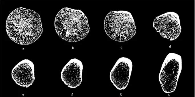
Figure 5 - Slices from a 3D µ-CT scan of a human femur bone spanning from the midsection of the femur head to the greater trochanteric area (a-h). Cortical Bone thickness is as low as 0.1 mm at the femur head (a), and
gets progressively thicker, up to 5 mm towards the interochanteric region (h)
The cervical region of the femur is characterized by a cortical bone thickness that progressively tapers until it reaches a minimum at the femur head. Hence, it is reasonable to state that the load is almost completely supported by trabecular tissue in this region [8].
As can been seen in figure 5 above (a), high density areas of spongy bone radiate through the femur head. These follow the main stress-lines in the neck and intertrochanteric regions (c, d) [40]. Cortical bone presents a high degree of structural organization, with several interlocking hierarchical levels.
6
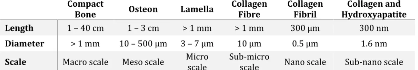
Compact
Bone Osteon Lamella Collagen Fibre Collagen Fibril Hydroxyapatite Collagen and
Length 1 – 40 cm 1 – 3 cm > 1 mm > 1 mm 300 µm 300 nm
Diameter > 1 mm 10 – 500 µm 3 – 7 µm 10 µm 0.5 µm 1.6 nm
Scale Macro scale Meso scale Micro scale Sub-micro scale Nano scale Sub-nano scale
Table 1 - Overview of the hierarchical levels of bone, together with size ranges of their structures
Figure 6 - Simplified representation of the compact bone structure at different hierarchical levels (above). Images representing each hierarchical level (below) [25, 47]
All of these structural organizations contribute to the peculiarities of bone, from the nanoscale up to the macro scale.
Cortical bone includes haversian structures (osteons), which are cylindrical structures 10 to 500 μm thick. In their centre, lies a cavity of about 20 μm wide, where blood vessels, nerves, and osteocyte processes run through.
The presence of haversian canals slightly worsens the mechanical properties of bone but is necessary to make space for nutrient and signal exchanges within the tissue. This raises
7 questions about why these particular structures are present, and how do they influence the delicate balance between stiffness and toughness which are crucial to this tissue. Transversally and diagonally to osteons, Volkmann canals (perforating canals) are found. These constitute connections from osteon to osteon and from osteon to periosteum (a connective tissue membrane that envelopes all bones and joints).
Haversian canals are immersed in the extracellular matrix and are delimited by cemented lines, which constitute pliable boundaries between the two.
The extracellular matrix on the outside of osteons is comprised of either primary bone or previous haversian structures which are being replaced by new ones. Osteon turnover is thought to maintain bone mechanical properties through time by replacing old structures that have accumulated damage at the microscopic scale [28].
The structural advantage of osteons comes from the organization at a lower hierarchical level, lamellae. Lamellae are organized as concentric sheets all around the central canal. Each osteon contains up to 20 concentric lamellae. Additional interstitial lamellae are found on the outside of haversian canals.
Each lamella has a preferential direction to its constituent fibres (collagen fibres), which is different from lamella to lamella. These are arranged diagonally around the central canal, wrapping around it in a staggered pattern: clockwise, counter clockwise, and clockwise again. A helicoidal structure is then formed, often compared to plywood, which raises mechanical properties of osteons considerably [34].
The helices formed by lamellae can present a higher or lower pitch in function of which stresses are present: tension leads to more relaxed helices, with longer fibres and small angles with respect to the principal axis, while compressive forces induce the opposite, with some cases in which fibres almost orthogonal to the principal axis [1].
Focusing on smaller scales, collagen fibres consist of packed bundles comprised of the even smaller collagen fibrils. These are shown to have characteristic diameters that correlate to the tissue’s ultimate tensile strength [9, 30].
8
Collagen fibrils themselves are constituted by nanoscopic HA platelets immersed in a collagen matrix. Hydroxyapatite only appears after the mineralization process in the shape of rod-like crystals.
HA crystals are distributed in an alternating fashion within the collagen matrix, periodically located along the fibril axis, with their long dimension parallel to the fibril axis.
1.2 Mechanics
At first approximation, human cortical bone can be considered as a linearly elastic material that fails at relatively small strains after exhibiting a well-marked yield point [21].
As usual for biological tissues, bone exhibits mechanical properties, which are dependent on the on direction of the applied load, i.e. anisotropic. Cortical bone anisotropy originates from the particular architecture of its small-scale components: from the peculiar shape of hydroxyapatite crystals and their spatial distribution inside the organic matrix, to the functionally oriented principal axis of osteons [23].
The different orientation of Haversian structure arises from the optimization of the bone architecture in order to sustain principal stresses during everyday load cycles. Due to this, in different bones, just as much as in different locations of the same bone, various orientations can be found.
Osteons’ longitudinal axis determines the major mechanical properties at the macroscopic level, and their general orientation tends to be roughly aligned with the principal stress directions. There also exists a difference between the circumferential and radial directions (with reference to a polar coordinate system placed in the femur as seen in figure 13), although much smaller with respect to the main axis. In addition, compact bone is stronger in compression than in tension.
Cortical bone shows relatively low mechanical properties when loaded in shear, and even worse in the transversal direction.
9 Various studies support the idea that the post-yield behaviour of this tissue is damage- [31, 37].
Strength-to-modulus ratio is an interesting index to understand the mechanical properties of bone. It is reported that this ratio is about 1.12 in compression and 0.78 in tension in the longitudinal direction of cortical bone [21].
Comparing the above to high-performance engineering materials such as Ti6Al1-4V alloys, typically used for hip prostheses, which shows a strength-to-modulus ratio of 0.50 to 0.73, it is quite higher for the bone tissue. Thus, Compact bone can be considered a high-performance material, particularly in compression.
At the Macro and mesoscale, a mechanical model that can suits cortical bone tissue is the orthotropic one. Orthotropy is a kind of anisotropy in which the compliance matrix has nine independent coefficients and three preferential directions, which are orthogonal to each other. Its compliance matrix is thus in the form of the Equation 1.
𝐶𝐶 = ⎣ ⎢ ⎢ ⎢ ⎢ ⎢ ⎢ ⎢ ⎢ ⎢ ⎢ ⎢ ⎢ ⎡ 𝐸𝐸1 1 − 𝜈𝜈21 𝐸𝐸2 − 𝜈𝜈31 𝐸𝐸3 0 0 0 −𝜈𝜈𝐸𝐸12 2 1 𝐸𝐸2 − 𝜈𝜈32 𝐸𝐸3 0 0 0 −𝜈𝜈𝐸𝐸13 2 − 𝜈𝜈23 𝐸𝐸2 1 𝐸𝐸3 0 0 0 0 0 0 𝐺𝐺1 23 0 0 0 0 0 0 𝐺𝐺1 31 0 0 0 0 0 0 𝐺𝐺1 12⎦ ⎥ ⎥ ⎥ ⎥ ⎥ ⎥ ⎥ ⎥ ⎥ ⎥ ⎥ ⎥ ⎤ (1)
10
Alternatively, a simpler model is the transversely isotropic one. It has infinite planes of symmetry and five independent variables shown in the Equation 2.
𝐶𝐶 = ⎣ ⎢ ⎢ ⎢ ⎢ ⎢ ⎢ ⎢ ⎢ ⎢ ⎢ ⎢ ⎢ ⎡ 1 𝐸𝐸1 − 𝜈𝜈21 𝐸𝐸2 − 𝜈𝜈31 𝐸𝐸3 0 0 0 −𝜈𝜈𝐸𝐸12 2 1 𝐸𝐸2 − 𝜈𝜈32 𝐸𝐸3 0 0 0 −𝜈𝜈𝐸𝐸13 2 − 𝜈𝜈23 𝐸𝐸2 1 𝐸𝐸3 0 0 0 0 0 0 𝐺𝐺1 23 0 0 0 0 0 0 𝐺𝐺1 23 0 0 0 0 0 0 2(1 + 𝜈𝜈𝐸𝐸 12) 1 ⎦ ⎥ ⎥ ⎥ ⎥ ⎥ ⎥ ⎥ ⎥ ⎥ ⎥ ⎥ ⎥ ⎤ (2)
At first approximation, the transversely isotropic model can also be applied to compact bone, given that the two non-longitudinal preferential directions show little differences in their engineering constants.
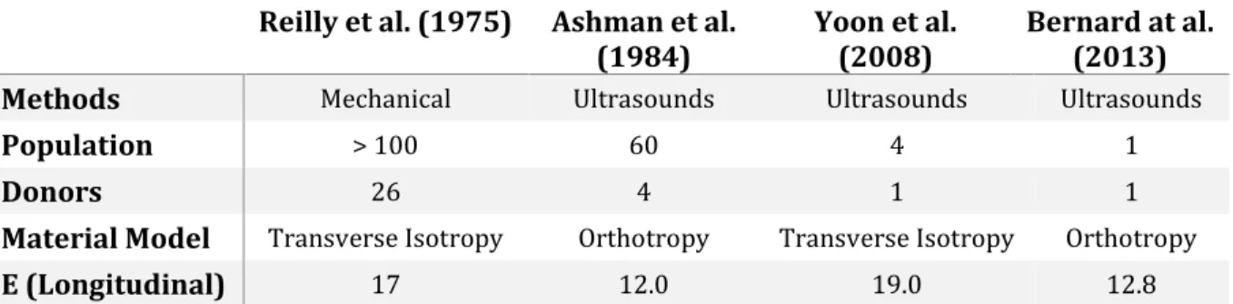
From the scientific literature, there exists great difference in the reported numeric values of these constants from study to study (table 2). This variability is dependent on a number of reasons: considered material model, analysis method, numerosity and peculiar characteristics of a given sample population, particular anatomical district from which samples are harvested, methods of sample processing before experiments, age and conservation of samples, and potential undetected anomalies or afflictions.
In the following table (table 2), some of these values are reported from four different studies.
11
Reilly et al. (1975) Ashman et al.
(1984) Yoon et al. (2008) Bernard at al. (2013)
Methods Mechanical Ultrasounds Ultrasounds Ultrasounds
Population > 100 60 4 1
Donors 26 4 1 1
Material Model Transverse Isotropy Orthotropy Transverse Isotropy Orthotropy
E (Longitudinal) 17 12.0 19.0 12.8
Table 2 - Numerical data Young’s Moduli measured from human femur diaphyses in the longitudinal direction of the bone. Methods, populations, and material models considered are reported as well [2, 3, 32,
46]
As can be inferred from the table 2, different studies have found quite different values for these moduli. It is to be noted that cortical bone is known to be highly heterogeneous between different anatomical sites. Samples from the femur shaft are expected to behave differently from ones from the neck and intertrochanteric regions.
Hence, numbers listed in the table are merely considered as reference values for the present study, while appreciably different ones are expected to be measured.
1.3 Toughness and Post-Yield Behaviour
As previously stated, compact bone shows an extraordinary fracture resistance compared to other materials with similar composition. Indeed, bone can rely on a broad degree of toughening mechanisms, ranging from the nanoscopic scale up to the macro scale, just as its structures’ hierarchical levels do. Moreover, bone is a living tissue, able to adapt and self-repair by renewing itself. All of the above make this hard tissue unique in its peculiar properties.
Fracture resistance is an essential characteristic for bone quality assessment; from it, one can evaluate bone fracture risk. In order to comprehend bone fracture toughness, it is necessary to look at each resistance mechanism at its specific hierarchical level [38].
12
Bone fracture is considered to be a mainly a strain-driven phenomenon [35, 48]; long bones generally break from bending or torsion or a combination of the two [30]. After micro fractures are formed, if not repaired quickly enough, total failure of the bone may happen. Mainly present at the micro scale and nano scale, in the following the fracture resistance mechanisms of the bone are listed [38]: Bone fracture is mainly a strain-driven phenomenon [35, 48]; long bones generally break from bending or torsion or a combination of the two [30]. After micro fractures are formed, if not repaired quickly enough, total failure of the bone may happen.
Mainly present at the micro scale and nano-scale, in the following the fracture resistance mechanisms of the bone are listed [38]:
1. Sacrificial bond breakage, molecular elongation, and intermolecular slipping. 2. Fibrillar slipping.
3. Crack deflection, both at the HA crystals and cemented lines scales.
4. Ligament and fibrillar bridging between crack boundary. Prevent further opening of the fracture keeping together the two edges.
5. Constrained microfracturing. Gaps formed by microfractures are quickly filled by collagen fibrils which curb further gap opening.
6. Sacrificial bond shattering at higher hierarchical levels such as fiber arrays of lamellae.
7. Cell fraction activity. Cell populations of the bone constantly repair crevices and openings that form in the bone tissue. Note that, although this is more of a repair mechanism than a toughening one, it still contributes to the overall toughness of the living tissue.
13
Figure 7 - Main toughening mechanisms found in the bone tissue. These go from the nanoscale to the macroscale and comprise a wide variety of structural organizations [38]
When bone tissue is subjected to an excessive load, intrinsic toughening mechanisms are the first to come into play: molecular uncoiling, intermolecular sliding, rupture of sacrificial bonds in the protein matrix, microcrack formation in the HA platelets, and fibrillar slipping. All these mechanisms comprise plastic deformation, and thus, energy dissipation.
14
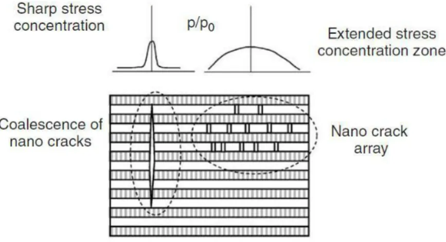
When the concentration of microcracks becomes too high, coalescence phenomena begin to occur, thus creating macroscopic cracks (figure 8).
Figure 8 - Visual representation of punctual and extensive damage to bone tissue at the nanoscale. A high enough number of nanocracks can fuse to form bigger gaps that lower
mechanical properties of the tissue [46]
Compact bone microstructure presents plenty of discontinuity features than can act as crack initiation sites, such as cemented lines and Haversian canals. On the other hand, all these structures serve as barriers as well, hindering or slowing down crack growth. Crack deflection can occur at different length scales, starting from the crystal platelet scale, in which microcracks offer a preferential line to crack advance (microcracks bridging) [38].
At higher scales, cement lines constitute a preferential path to the progress of cracks as well. These are thus deflected around osteons and pass through their layered net instead [25]. This is considered to be a repair mechanism that speeds up healing, given that most of the bone cell fraction lies within osteonal structures [39].
Due to the above-mentioned mechanisms, when a microfracture is formed, its progress is greatly dependent on the anatomic region in which it has formed, or in other terms, on the osteon density of the location.
An increase of the crack path translates into an increase in the amount of energy required to break the tissue, and thus, in greater material toughness.
15 At the same hierarchical level, thanks to the specific lamellar structure of the bone tissue, crack bridging happens because of unbroken collagen fibres, which prevent further opening of the fracture.
Contrary to what would be expected, given that bone is predominantly comprised of a fragile material, it presents an outstanding fracture resistance thanks to this intricate net of toughening mechanisms. This is why an elevated number of studies are currently trying to emulate its properties through biomimetic strategies.
Figure 9 - Schematization of crack progress within osteonal structures. Note that multiple micro cracks form at the tip of the rupture, and that these are deflected extensively thanks
to the bone structure [25]
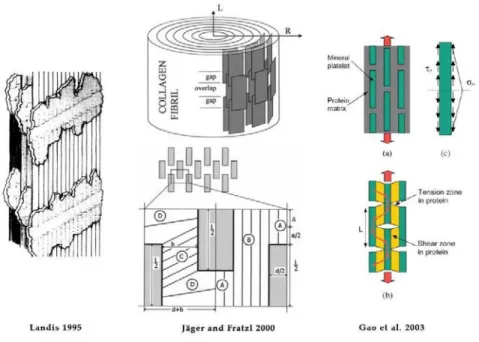
Considering the nanoscopic hierarchical level, a two-dimensional model, the Jäger and
Fratzl model, exemplifies the bone matrix as intercalated rectangular platelets immersed
16
Figure 10 - Display of the main nano scale structures utilized for mathematical modelling of the bone tissue mechanics
This simplification can shed light as to how the bone composite material works.
Given that there exists a mismatch of three orders of magnitude between the mineral phase and the collagen matrix Young’s moduli, it is hypothesized that all the load applied to the tissue is supported by the mineral phase, while the collagen matrix transfers load from platelet to platelet under the form of shear [20].
This particular disposition of the two phases allows, on the one hand, for the soft component to support high loads without straining excessively, and on the other it allows for the brittle phase to resist damage thanks to absorption of much of the crack energy that would otherwise progress unhindered through its whole thickness.
One possible interpretation of the interactions between the two is that the soft phase forms some sort of sheath around the hard crystals, distributing load evenly on their surfaces, and preventing localized stress peaks that would otherwise break them.
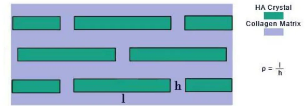
The Jäger and Fratzl model enables to visualize better how the two phases interact with each other [18]. Two factors have been found to be crucial while studying this tissue: the amount of crystal platelets with respect to the cross-section of the bone, and the platelet
17 aspect ratio [20]. The former is important because HA behaves in a brittle manner, and thus, completely snaps when a crack forms, and more crystals through the cross-section means that more cracks need to start for the bone to completely fail. The latter is the average crystal aspect ratio ρ=l/h, where l is the crystal length, and h is its thickness. It has been found that the higher this geometric parameter (ρ) is, the greater the composite material stiffness (with constant volume fractions). Small imperfections in the crystalline structure appear to become less important when ρ reaches a value of “flaw tolerance”, for which crystal platelets rupture at their theoretical strength values [14].
Figure 11 - Nanoscopic 2D model of HA/collagen composite. l and h are the length and thickness of crystal platelets, while ρ is their ratio
The aspect ratio is reported to be between 10 and 100 being HA crystal 100 to 500 nm long. In their study, Ji and Gao have also demonstrated that this is an ideal length range for the crack toughness to be the closest to its theoretical value as possible. This also clarifies why the hierarchical level of bone starts at the nanoscale and not at a larger one.
Thanks to this unique structure and its ability in distributing forces, compact bone exhibits an unexpectedly high Young’s modulus.
As previously written, it is composed of 40-45% volumetric fraction of hydroxyapatite, and the remaining 50-60% of collagen-like proteins. Collagen has a Young’s modulus reaching a maximum of 100 MPa, while hydroxyapatite up to 100 GPa.
Bone tissue, derived by their combination, presents 10-20 GPa of Young’s modulus, smaller than pure HA, but, considering stoichiometry, at a much closer magnitude to the
18
mineral phase than the organic one. This small reduction in modulus -which is due to the presence of collagen instead of pure HA within the tissue- is needed in order to enhance strength and crack resistance; In fact, bone tissue strength in tension reaches up to 100 mJ/mm3 while its components are in the order of a few tens of MPa [20, 49].
Compact bone is composed of polymeric matrix, thus exhibiting time-dependent properties as polymeric materials usually do. Loading rate is therefore a crucial parameter in the fracture behaviour: higher strain rates lead to brittle fractures, while lower velocities allow for more ductile responses.
This can be seen on a typical stress/strain plot, which exhibit a higher slope and failure at smaller strains as the strain rate.
Figure 12 - Typical stress/strain curves for human cortical specimens parametrized for strain rate [1/s] [21]
An appropriate loading rate is to be chosen in order not to induce stiffening in samples; this will be addressed during the design of the test.
19
1.4 Aim of the Study
The skeleton apparatus plays an essential role in the human body. Its main functions comprise -but are not limited to- supporting the body’s own weight, enabling locomotion and movement, providing anchoring for muscles and tendons, framing body shapes, and constituting a reservoir for mineral ions homeostasis in the body.
All bones have to adapt to the specific arrays of force distributions they encounter on a day-by-day basis such as gait, standing, jumps and sprints, or even more sporadically as in the case of accidental events.
The femur is the largest-long bone of the human anatomy. Skeletal muscles in the thigh and gluteus exert the vast majority of forces necessary for locomotion by acting on the femur [39].
Given that the femur is subjected to extremely high forces (during intense activities load can reach several times the individual's own body weight), it shows a particularly high degree of adaptation to stresses, aimed at increasing its resilience and overall fracture toughness [17].
One of the most common fractures that affect the femur happens either on its cervical or interochanteric regions, often following a traumatic event such as falls from the upright position [16]. Such an event happens with a magnitude of force, among other factors, directly related the body weight of the person and height of the fall itself. Moreover, forces generated during accidents tend not to be aligned to the longitudinal axis, the direction in which long bones present the highest mechanical properties [21].
Bone tissue diseases increase fracture risk factors considerably. Among these, osteoporosis constitutes the greatest threat, both because it diminishes overall bone density and because it compromises overall tissue quality [11]. This condition, at later stages of the pathology, can cause fractures not only because of accidental events, but also upon the application of physiological loads.
Going through census data, it has been reported that, from 1999 to 2002 in Italy, there have been 80.000 hospitalizations due to hip fractures -about 20.000 per year- mainly located in the femur neck area, and with a higher incidence for the elderly and those
20
suffering from osteoporosis [36]. In 2008, in the United States, 341.000 cases were reported [22].
Proximal Femur fractures are extremely distressing in affected subjects, which are predominantly females over the age of 70 [16]. For the elderly, the weakening of the bone due to illness plays a major role in their risk factor [8, 42].
Mechanical properties of bone tissue -with particular reference to the femoral anatomic region- are, therefore, of clinical relevance.
Cortical bone is an anisotropic material [21], which is quite convenient for long bones, such as the femur, because it enhances its mechanical properties with specific reference to the main direction of the applied load. Many studies in the past have analysed the femur’s mechanical properties by harvesting samples from the diaphysis [32, 40, 47] while far less have focused their attention to its cervical region [4, 8, 19]. Here, the burden on the bone and its geometry are quite different from the diaphysis, and thus different properties are expected.
The main clinical problem is the lack of experimental data on this particular region. Here, difficulties in the extraction of samples has often deterred scientific investigations, which possibly explains the above-mentioned lack in quantitative information.
Therefore, the objective of this study is to develop an experimental procedure which is aimed at filling the above-mentioned gap. In particular, the experimental procedure will be used to achieve preliminary results for the mechanical characterization of the cortical bone in the cervical region of human femurs. This would show the feasibility of further, deeper studies which would have clinical relevance.
In the present study a newly-developed harvesting methodology paired to a suitable three-point bending setup will be proposed, specifically designed for this peculiar region. The femoral neck region is extracted from the rest of the bone by means of two parallels cuts 25 mm away from each other. The isolated part is clamped in the specific support and sliced through the use of a Microtome. An average of 7 slices 1 mm thick can be obtained from each aspect of the neck (lateral and medial). Then, raw slices are machined into
21 prismatic shapes by means of a precision sander down to the final nominal geometry: 0.4 x 1 x 10 mm. Finished specimens are then frozen.
Before carrying out the mechanical test, samples are thawed and their size is measured using a 3D Measuring Laser Microscope; samples are subsequently rehydrated in saline solution for 20 minutes long at room temperature.
Samples are then set on the three-point bending apparatus; synchronized image acquisition and load recording are carried out during tests, in order to obtain time-arrays comprised of displacement values coupled with loads. More precisely, the instantaneous displacement is measured with respect the central point of the beam by means of a tracking software. Force/displacement data are converted to stress/strain values in order to obtain the engineering constants of interest.
The above procedure will be addressed in Chapter 2, during which sample preparation and testing procedures are reported, together with accuracy and repeatability assessment. In the third and final chapter, results will be reported, followed by thorough discussions and conclusions.
22
Chapter 2: Materials & Methods
The following chapter is comprised of two sections: the first reports sample harvesting and preparation, while the second describes their mechanical testing.
During the first half of the chapter, a series of preliminary considerations regarding the harvesting procedure are made, followed by the description of the target shape and size for the specimens. The equipment utilized during sample preparation are described, before thoroughly reporting each of the steps followed during the harvesting procedure. This is done in order to allow for possible future reproductions of the methods.
In the second half, the testing setup is reported, together with the description of the purposely-made components for the present study. Then, specifications about the parameters used to carry out the samples mechanical characterization are reported. Subsequently, a series of tests in order to assess the goodness of the whole procedure are presented in the Accuracy and Repeatability paragraph. These are carried out with samples harvested from swine, and from a well-known aluminium alloy (6060 T6).
2.1 Sample preparation
Preliminary considerations
Because of the lack in the scientific literature about the extraction and preparation of cortical bone samples from the femoral neck region, previous studies made on the same bone’s diaphysis have been taken as reference.
Throughout scientific literature, the golden standard regarding bone tissue processing comprises using low-speed diamond saw-blades in wet conditions followed by high-grit sanding [19]. Cuts have to be sharp and precise, as obtaining regular shapes is of utmost importance. Therefore, the majority of sawing setups have guides for cuts, which are generally fixed to the sample, and limit one or more degrees of freedom. This means that a suitable fixation method needs to be found that doesn’t interfere with tests and does not
23 damage sample tissue, or if it does so, damage must be restricted to areas of no interest. Clamps and interlocks are the usual solution for this. On the other hand, plenty of studies implement cement glues for fixation. This method is not considered suitable for the present study, as heat generated during polymerization might denature the protein content of samples. Proteins start to denature at temperatures as low as 55 °C [24].
Saws are generally utilized at low speeds and under wet conditions. This is because friction generates heat which may affect the mechanical properties of the tissue.
Low speeds help by diminishing friction heat, while water or substitutes work by dissipating generated heat.
Sanding is the final step as it enables the operator to smooth out surfaces and eliminate grooves and ridges which are typically left after sawing and which can constitute crack initiation sites. Sanding is generally performed under wet conditions and with high-grit sandpapers.
Grinding apparatuses generally comprise some mechanism that continuously changes the direction in which abrasion is performed in order to achieve better results. Continuous grinding in only one direction introduces errors, portions of the sanded surface that are antiparallel to the grinding direction become kinked as they are subjected to a higher degree of abrasion.
The objective is to obtain straight, smooth surfaces, that resemble the ideal prismatic shape as much as possible.
Cortical bone is generally harvested from easily accessible anatomical districts, either big, flat bones as in the case of the iliac crests or from the midsection of long bones such as the femur. This is because these regions are large enough to provide a higher number of samples and are easier to work and allow for bigger specimens to be obtained, compared to thin/small regions such as the femur neck. Results from these specimens, as stated in the previous chapter, are not expected to represent the mechanical behaviour of samples originating from other portions of the same bones. The present study will focus on extracting samples that better represent the mechanical behaviour of the cortical bone
24
tissue in the femur neck instead of trying to obtain an elevated number of specimens from the femur shaft.
Regarding tissue preservation methods, fresh-frozen tissues are almost universally utilized. All preservation methods impair the mechanical behaviour of the tissue. There is evidence that alcohol and formaldehyde both cause severe damage to the collagen phase in the bone by dehydrating it, while freezing causes minor damage and does not impair results [42]. What is to be avoided, in the case of fresh frozen specimens, is repeated freeze-thaw cycles that will lead to an accumulation of damage within the tissue and thus result in non-reliable data.
All of the above has been adopted for the current study. Nonetheless, some aspects of the design have to be addressed differently in order to obtain a better suited procedure for the femur neck.
Because of the nature of the harvesting site, bone-shaped specimens -the preferred shape for normal tensile tests- are excluded, as their geometry would limit the number of samples obtainable from each donor, as well as making the harvesting procedure more difficult, especially in the osteoporotic and diseased individuals. Furthermore, Compact bone generally forms only a thin wall in the femur neck, with normal values ranging from 1,5 mm on the medial side to as little as 0,4 mm on its lateral aspect (in the healthy subject). Given this, a prismatic shape is considered as the most appropriate choice.
Prismatic specimens can be easily tested either in a three-point or four-point configuration, with the latter being the best choice. In a four-point bending test the central section is uniformly subjected to the maximum bending moment; this guarantees a uniform stress distribution along this region, which translates into better statistical results. In contrast, during a three-point test only the critical point is put under the maximum stress value, due to the linear momentum distribution along the sample length. However, in this specific case, sample length is limited because of the geometry, as can be inferred from the below image (figure 13); this do not allow for a four-point bending setup, and thus, a three-point bending test is chosen instead.
25 Focusing on the specimen’s dimensions, the size range that can be obtained from a femur’s cervical region is quite restricted. This is mainly due to the fact that cortical bone is thin and that it presents a high degree of curvature around its longitudinal axis, meaning that samples cannot be too thick nor too wide (with respect the radial and the circumferential directions – “R” and “C” in figure 13). Adding to this, there exists a second, generally less pronounced saddle on the supero-lateral side of the neck. Its shape and degree of curvature has been observed to be quite variable.
Figure 13 - Three-dimensional model of a femur neck showing the cervical region with a cylindrical reference system; longitudinal (L), radial (R) and circumferential (C) directions
are defined as shown
For this reason, during the first phases of the study, two three-dimensional images obtained from computer micro-tomography have been analysed in order to understand the range of the specimen size obtainable from the region of interest. The two virtual models have been processed with the aid of Fiji (National Institute of Health), Autodesk
Meshmixer, and Autodesk Fusion 360 in order to simulate and idealized the cutting process
26
Image processing has been conducted as follows: Fiji’s 3D median noise filter has been applied twice, with a cut-off radius of two pixels in order to eliminate all non-connected data from the image. In doing so, the trabecular portion of each slice is removed without affecting the cortical thickness in any way.
Then, the DICOM sequences have been imported in Meshmixer as .stl files; plane cut tools have been utilized to isolate the area of interest, and the remaining trabecular structures have been manually polished away with smoothing tools. Ultimately, files have been worked in Fusion 360 where typical slicing and sanding procedures have been reproduced with Boolean operations so that details such as blade thickness could be taken into account. The maximum specimen size obtained from the above three-dimensional models has been of 2.85 x 1.23 x 10.51 mm.
One of the main concerns was about sample length, because, the shorter the sample, the higher the number of specimens that can be obtained from a single slice.
On the other hand, the precision load cell utilized in the current study has a maximum load of 5 N; in order to maintain the force required to analyse our samples under the cell limit, it has been chosen to act on their thickness. In order to compute the maximum thickness for the specimen that our system is capable of withstanding, the mathematical model of the three-point bending for a prismatic beam has been implemented.
ℎ𝑚𝑚𝑚𝑚𝑚𝑚 = �2𝑏𝑏𝜎𝜎3𝐹𝐹𝐹𝐹
𝑚𝑚𝑚𝑚𝑚𝑚 (3)
An ultimate strength of 135 MPa has been considered as the mean value for 𝜎𝜎max, according
to the literature [21, 33].
Supposing that the range of possible specimen sizes calculated using the micro-CT analysis is reliable, the trade-off between sample dimensioning and total specimen number is addressed. Bigger specimens are easier to work, but inevitably limit the number obtainable from each human donor. Thus, the circumferential size b has been set equal to 1 mm, an in-between value that is neither too wide nor too narrow.
27 Regarding sample length, its maximum achievable value is supposed to be about 10 mm, because of the naturally occurring longitudinal curvature of the bone in this anatomical district. From the above value, a total of 2 mm will be used as supports near to the endpoints of each sample, and, thus, the final test span l is about 8 mm. Given that femoral neck are generally longer than 20 mm, the possibility of creating two samples through the length of the neck becomes available. This would double the number of obtained specimens.
A force F of 3.5 N is considered. This is the maximum withstanding load of the cell (5 N) reduced by a 30% safety factor.
According to the equation 3 and to the above considerations, the upper limit for the samples’ height h has been set to 0.5 mm. In figure 14, a schematic representation of the final shape and dimensions set as target can be observed.
Figure 14 - Schematic representation of the sample’s final shape. Length (l) is 10 mm, width (b) is 1 mm, and height (or thickness) (h) is 0.5 mm
In order to achieve sample target shape and size, two different extraction procedures have been investigated in order to reach an optimal harvesting technique: core drilling and microtome slicing.
The method that better suits this particular problem has been chosen by means of a series of selection criteria: obtaining high quality specimens, with smooth, regular surfaces, and without variations along their length; gathering the maximum number of samples within the area of interest; completing the overall process in the shortest amount of time in order
28
not to let tissue samples dehydrate or even decay. Moreover, samples should not be thawed and frozen repeatedly.
Preliminary harvesting tests have been conducted on swine samples. Their cortical tissue is comprised of a fibro-lamellar structure similar to human bone [12]. However, there exist a few substantial differences: animal bones are differently shaped and sized, and typically present distinct mechanical properties from human bones, mainly derived from different mineralization levels. These factors have to be taken into account once the final cutting strategy is outlined.
Core drilling has been considered because it simplifies the overall extraction process and enables a faster specimen harvesting. On the downside though, it presents many drawbacks as it leads to a higher amount of wasted material. Difficulties are found in obtaining a clean, regular cylindrical geometry due to the small cortical thickness of this anatomical region, and the struggle in orientating the curved tissue with respect the straight axis of the core drill bits.
29 Although microtome slicing requires a more laborious procedure in order to grip the femur cervical region in the microtome vice, the final results are of much higher quality. First and foremost, loss of material is strongly reduced; the overall procedure has shown to be more reproducible and reliable; a higher number of samples can be obtained from the same region. Furthermore, the sanding process is simplified thanks to the presence of two straight parallel flat faces, which can be used as grip areas.
Given the above, the microtome slicing procedure has been selected.
Once a first harvesting procedure has been defined for swine samples, additional testing on three alcohol preserved human femora has been done in order to verify that the procedure tested on animal tissues is actually valid for the human case. These are not suitable to be included in the experimental campaign as they have been preserved in alcohol solution for extended periods of time. Thus, they have compromised mechanical properties, mostly because of the denaturation of the protein fraction [42]. Their usefulness lies in the possibility of verifying the feasibility of the harvesting procedure, as well as confirming the obtainable sizes with the real anatomical geometry that will be found during the final sample extraction.
This last step has confirmed the viability for the cutting and sanding processes with the exact geometry of the human femur.
Slicing
The harvesting procedure utilized to obtain samples from human femurs is detailed in the following:
The first step in the harvesting procedure involves isolating the cervical region. This is done by means of the Cut-off metallography machine (Remet TR 60) used to create two parallel cuts just above and below the femur neck in the transversal plane (see figure 16). Both cutting sites have to be unequivocally identified.
This procedure must exclude the curved portion of the femur head, in order to increase the maximum specimen length achievable, namely, the slated junction between the head
30
and neck. This requires setting a unique geometrical reference, suitable for all sizes and proportions that a femur may present.
The head diameter has been chosen as characteristic dimension for this purpose; its value is measured and multiplied by a factor of 0.2, obtaining the length defined as x (figure 16). The first cut is made moving distally along the longitudinal direction (with respect to the femur neck), starting from the head limit by the exact amount of x. The head limit is clearly visible because of the presence of cartilaginous tissue
Figure 16 - Harvesting procedure. Frozen proximal femurs are cleaned-off soft tissues (a). The head diameter is measured and multiplied by a factor of 0.2, forming the length x (b). X
is used as the distance between the head (demarcated by the presence of cartilage, yellow line above) and a first cross-section of the neck, which is orthogonal to its longitudinal axis (orange plane in the picture) (c). Maintaining the same spatial orientation, a second cross-section is marked 25 mm down towards the distal end of the bone (blue in the image) (d).
31 The second cut is made 25 mm down in the same direction. The resulting shape is shown in figure 16 “h”. The above length is enough to include the whole neck area of a typical human, excluding the greater trochanter. The medial and lateral aspects are then separated by means of a longitudinal antero-posterior cut. In order to be able to identify the region from which samples will be harvested, a central line is marked using permanent ink (figure 16 “e”).
The next step provides the actual slicing of the isolated region, by means of the Leica
SP1600 Saw Microtome. The microtome is composed of the following parts: a central rod,
on which samples are mounted (figure 17 “C”); a ring-like diamond blade with a 0.3 mm thickness (figure 17 “B”), that has its cutting edge facing towards its inside; a micrometre screw (figure 17 “A”), that allows to move up and down the central rod, orthogonally with respect to the fixed blade.
In order to firmly fix samples during the cutting procedure, an appropriate aluminium vice has been designed.
Figure 17 - Microtome setup. The micrometre screw (A) is used by the operator in order to set the slicing height. The blade diameter (B) in the internal diameter of the cutting edge. This limits the girth of the
32
Plenty of restrictions and requirements have to be applied to the vice’s design. First and foremost, the micrometre screw range is quite limited, enabling only a 1.2 cm scope. This limits the height of the femoral neck region that can be gripped by the vice. Then comes the relatively meagre internal diameter of the blade (about 8 cm) that might obstruct vice insertion at the centre of the apparatus, together with the horizontal run that the circular blade can cover without sawing the aluminum support. The final geometry of the vice can be seen in figure 18.
The vice can be closed by means of two lateral screws (A). The femoral neck is gripped on its proximal and distal ends by the two parallel gripping faces (B). Tightening of the vice can cause damage of the compressed tissue area, and even more so, for the existing thin cortical layer. Given that the anterior and posterior regions are not of interest for the present study, they can be clamped forcefully, and thus, sacrificed in order to properly secure the femoral neck. A large enough portion of each cervical region must be held in the vice in order not to risk breakage of the clamped region, an event that would result in a loss of tissue. Clamping strength must be high enough, to avoid tilting of the sample, or even worse, in the complete loss of grip on the wet bone.
33
Figure 18 - Microtome grip. This component is fixed to the whole apparatus by means of the dovetail shown in figure 17 (C). Two screws (A) secure the sample by tightening the gripping faces (B). In the
image above there can be seen a typical half of a femur neck clamped in its posterior region
The whole body of the aluminum vice is designed in order to fit the internal diameter of the microtome blade, with its clamps completely laying under it, even when the micrometre screw reaches its upper scope limit.
The sample is then firmly fixed to the microtome vice, always keeping note of the anterior and posterior orientations.
Slicing is done as described in the following steps: the vice is inserted into the microtome, and the previously marked midline of the sample is aligned with the circular blade with the aid of the micrometre screw; the blade is brought toward the top of the sample in steps 1.3 mm long each, up to the maximum number of integer steps that the screw scope allows to reach. the choice of 1.3 mm long steps is made because it is the result of the sum of the target sample width (1 mm) plus the blade thickness (0.3 mm); cutting starts using low speeds both for the blade spin and for the pushing arm in order not to risk protein
34
denaturation or breakage in the tissue; after each cut, newly formed slice is removed, registered, and marked in its proximal end in order not to lose traceability.
Figure 19 - Harvesting procedure: a longitudinal cut (b) separates the supero-lateral and infero-medial halves (c). A central midline is found and marked as “0” (d), used as reference
point for specimen tagging. Central, anterior and posterior slices are cut for each medial and lateral region (f)
Raw slices obtained from the microtome present a long, slender, and curved geometry; thus, they are divided into their relatively proximal and distal parts. This manual cut simplifies the subsequent sanding procedure, better accommodating the curvature on each half of the slice and doubling the total number of samples obtainable from each slice. A minimum length of about 8.5 mm is kept for all specimens.
Most of the trabecular bone is manually removed from each slice, before proceeding to the sanding procedure.
35
Figure 20 - Proximal half of a typical slice obtained at the end of the microtome cutting procedure
Sanding
Once extraction and cutting of samples have been completed, each slice undergoes the sanding process, at the end of which the raw slice is shaped into a regular prismatic geometry.
An EXAKT 400CS Micro Grinding System has been utilized as sanding apparatus, which is comprised of a rotating disk on which sanding paper is set. A press gently pushes the sample on the rough surface by means of weights, while a steam of fresh water guarantees that the process occurs in wet conditions.
The press is moved in a see-saw-like movement, which is a cyclic motion that guarantees an overall better result as a more uniform grinding is performed on the surface. This translates into straighter faces and sharper edges.
Plexiglas dishes are fixed to the press thanks to a vacuum pump that creates suction on them. These can be used in turn to fix different sized and shaped samples on the sander. A micrometre screw gauge enables fine-tuning of the sanding process down to a hundredth of a millimetre.

![Figure 12 - Typical stress/strain curves for human cortical specimens parametrized for strain rate [1/s] [21]](https://thumb-eu.123doks.com/thumbv2/123dokorg/7505397.104809/32.918.295.657.478.731/figure-typical-stress-strain-curves-cortical-specimens-parametrized.webp)
