Interpretable statistics for complex modelling: quantile and topological learning

(1)

S

APIENZA

U

NIVERSITY OF

R

OME

D

OCTORAL

T

HESIS

Interpretable statistics for complex

modelling:

quantile and topological learning

Candidate:

Tullia PADELLINI

Supervisor:

Pierpaolo BRUTTI

Scuola di Dottorato “Scienze Statistiche”

Curriculum Methodological Statistics

Department of Statistical Sciences

(2)

(3)

Abstract

As the complexity of our data increased exponentially in the last decades, so has our need for interpretable features. This thesis revolves around two paradigms to approach this quest for insights.

In the first part we focus on parametric models, where the problem of interpretabil-ity can be seen as a “parametrization selection”. We introduce a quantile-centric parametrization and we show the advantages of our proposal in the context of regres-sion, where it allows to bridge the gap between classical generalized linear (mixed) models and increasingly popular quantile methods.

The second part of the thesis, concerned with topological learning, tackles the problem from a non-parametric perspective. As topology can be thought of as a way of characterizing data in terms of their connectivity structure, it allows to represent complex and possibly high dimensional through few features, such as the number of connected components, loops and voids. We illustrate how the emerging branch of statistics devoted to recovering topological structures in the data, Topological Data Analysis, can be exploited both for exploratory and inferential purposes with a special emphasis on kernels that preserve the topological information in the data.

Finally, we show with an application how these two approaches can borrow strength from one another in the identification and description of brain activity through fMRI data from the ABIDE project.

Acknowledgements

I am forever in debt with Håvard Rue for his help and his hospitality. I would also like to acknowledge Peter Congdon for providing the hospitalization for self harm data used in Section 1.7.1 and Bertrand Michel for referring to the Fullerenes analysed in Section 3.2.

Special thanks go to the reviewers Massimo Ventrucci and Larry Wasserman for their valuable comments and constructive feedback.

(6)

(7)

Introduction

This thesis is based on two main pillars: Quantile Regression and Topological Data Analysis.

Quantile Learning The first part of the thesis revolves around Quantile Regression, a

supervised technique aimed at modeling the quantiles of the conditional distribution of some response variable. With respect to “standard” regression, which is concerned with modeling the conditional mean, Quantile Regression is especially useful when the tails of the distribution are of interest, as for example when the focus is on extreme behavior rather than average, or when it is important to assess whether or not covariates affect uniformly different levels of the population.

Even though the idea dates back to Galton (1883) (as noted in Gilchrist (2008)), Quantile Regression was formally introduced only relatively recently by Koenker and Bassett (1978). Since then, the use of quantiles in regression problems has seen an impressive growth and has been thoroughly explored in both the parametric (see Yue and Rue (2011), Wang, McKeague, and Qian (2017)), and non-parametric framework (see Yu and Jones (1998), Takeuchi et al. (2005), Li and Racine (2007)) with applications ranging from the Random Forest Quantile

Regression of Meinshausen (2006) to D-vine copulas for quantiles in Kraus and Czado (2017), through Quantile Regression in graphical models as in Ali, Kolter, and Tibshirani (2016).

One of the most significant developments in the Quantile Regression literature has been the introduction of the Asymmetric Laplace Distribution (ALD) as a working likelihood Yu and Moyeed (2001). From a frequentist point of view, the use of the ALD gave rise to a class of likelihood based method for fitting quantile models and has been instrumental in introducing random effects in linear and non linear Quantile Regression models; see for example Geraci and Bottai (2007), Geraci and Bottai (2014), Geraci (2017) or Marino and Farcomeni (2015) for a more comprehensive review. The introduction of the ALD has been even more critical in the Bayesian framework, where the likelihood is required in inferential procedure Yu and Moyeed (2001). As a result, fully bayesian versions of Quantile Regression, such as the additive mixed Quantile model of Yue and Rue (2011), as well as Quantile Bayesian Lasso and Quantile Bayesian Elastic Net, have been developed in the last couple of years, examples being Alhamzawi, Yu, and Benoit (2012) or Li, Xiy, and Lin (2010). Extensions of the Asymmetric Laplace Distribution such as the Asymmetric Laplace Process (Lum and Gelfand (2012)), broadened Quantile Regression to spatially dependent data.

Despite their popularity however, ALD based methods are not always satisfactory, especially in terms of uncertainty quantification. The use of the ALD introduces an unidentifiable parameter in the posterior variance, hence any inference beside point estimation is precluded (Yang, Wang, and He 2016).

(8)

We propose a model-based approach for Quantile Regression that considers quantiles of the generating distribution directly, and thus allows for a proper uncertainty quantification. We then create a link between Quantile Regression and generalized linear models by mapping the quantiles to the parameter of the response variable. This formulation not only recast Quantile Regression in a much more cohesive setting and overcomes the fragmentation that characterizes the Quantile Regression literature, but it is also key to an efficient and ready-to-use fitting procedure, as the connection allows to estimate the model using R-INLA (Rue, Martino, and Chopin (2009) and Rue et al. (2017)).

Additionally, we extend our model based approach in the case of discrete responses, where there is no 1-to-1 relationship between quantiles and distribution’s parameter, by introducing continuous generalizations of the most common discrete variables (Poisson, Binomial and Negative Binomial) to be exploited in the fitting.

Topological Learning In the second part of the thesis we focus on Topological Data

Analysis (TDA), a rapidly growing branch of statistics whose aim is estimating topological invariants of unobserved manifolds, typically (but not exclusively) through point–clouds sampled on them. TDA can be seen as a way of uncovering the “shape of the data” in terms of their topology. As topology is a rather broad definition of shape, which is focused on the connectivity structure, TDA methods are intrinsically related with clustering, making them a great exploratory tool for high dimensional and highly complex data.

TDA has a relatively short history, being based on Persistent Homology Groups, topo-logical invariants introduced only at the beginning of 2000 by Edelsbrunner, Letscher, and Zomorodian (2002). The main tool of this class of methods, the Persistence Diagram, a topological summary containing both topological features and a measure of their importance, has been investigated from a statistical perspective even more recently (B. T. Fasy et al. 2014, Chazal, Glisse, et al. (2015)). While doing statistics on the Persistence Diagram has yield positive results (Chazal, Fasy, et al. 2015), statistics using the Persistence Diagram has proven to be more challenging, as even basic quantities such as the mean are not easy to compute or to interpret (Turner et al. 2014). For this reason several alternative representation of the Diagram, typically in the form of functional object, have been proposed (Bubenik (2015), Adams et al. (2017) or Moon, Giansiracusa, and Lazar (2018) to name a

few examples).

We introduce a new topological summary for scale-spaces, the Persistence Flamelet, which allows to extend TDA to the case of object that have multiple resolution, such as time series, which depend on time, or smoothers in general, which involve a tuning parameter. We investigate in particular the case of kernel density estimators, where the scale parameter is the bandwidth, and we show how its topology changes with it. We prove that the Flamelet is not just a visualization tool by characterizing it probabilistically and showing that Central Limit Theorem and Law of Large Numbers hold for this new object.

Even though the impressive growth of TDA literature in the last couple of years has yield several inference–ready tools, this hype has not yet been matched by popularity in the

(9)

3 Quantile Regression Topological Data Analysis

Inferential Approach Bayesian Frequentist

Computation Fast Slow

Field Traditional Statistics Borderline Statistics

practice of data analysis, we thus focus on the potential of topological characterization as a Learning tool, with a special emphasis on Supervised problems. In order to perform inference using topological summaries, which are typically defined in spaces which are not amenable to direct modelling, we adopt a kernel approach to recast the learning into more familiar vector spaces. We define a topological exponential kernel, we characterize it, and we show that, despite not being positive semi-definite, it can be successfully used in regression and classification tasks. We examine in particular the former and we show how to use Persistence Diagram as covariate and as responses in regression problems. Finally, we show preliminary, yet encouraging, results of combining quantile methods with TDA to gain insights on brain activity. Building on functional connectivity, which in the literature has been analysed mostly with respect to its 0-dimensional structure, we show how TDA allows straightforwardly to investigate higher dimensional features as well, and then we use the quantile methods introduced in the first part of the thesis to better understand phenotypical determinants of the topological structure.

A tale of two thesis? At a first glance, there is little in common between the two

topics themselves, as Quantile Regression is well established in “classical” statistics, while Topological Data Analysis is an emerging research area at the boundary between Statistics and Computational Topology. Our contributions also appear to go in opposite direction, since we approach Quantile Regression from a model-based perspective, heavily relying on parametric modelling to exploit fast and efficient Bayesian fitting procedure (INLA), while we opt for a parameter-free approach for Topological Inference, adopting classical tools in non-parametric statistics such as kernels. Finally, from a computational standpoint, thanks to INLA, we are providing extremely efficient and extremely fast implementations in the Quantile Regression setting, while, due to the indefiniteness of topological kernels, we turn to non-efficient solvers for classification problems using topological summaries, whose computation is already very time-consuming.

At a closer look however, the contribution presented in this thesis are all trying to pursue the same goal, that is interpretable characterization of data. Despite being at the core of learning, interpretability is in fact not a uniquely defined concept but there are many different declinations of this notion, depending on the task and most importantly on the information already available. Our contribution can be seen as as an attempt to enforce interpretability at the two end of the spectrum of model knowledge, i.e. the case where we know almost everything (that is, we have a parametric model for our data) and the case we know almost nothing (i.e. we don’t even know the support of the data generating process). From a parametric perspective, the interpretation typically goes through the parameters. Our model-based approach to Quantile Regression can be thought of a way of reparametrizing the model in terms of its quantiles. While the mean needs not to exist, the quantile are always defined and they retain the same interpretation regardless of the complexity of the

(10)

model considered, hence a parametrization in terms of quantiles can be thought of as a “universal” parametrization.

The main argument against a parametrization based on quantiles may be that in the discrete case quantiles still exist but are not unique, which is why we focus on the discrete case, proposing a model-aware approach to overrule this objection.

As for the case where preliminary information is close to null, there may be even too many ways of finding a meaningful characterization of data, but topological invariants stand out for many reasons. The main one is of course their interpretability and the relevance of such interpretable objects in statistical learning: topological features of dimension 0, connected components, can in fact be thought of as clusters or peaks, while topological features of dimension 1, loops, represent periodic structures. Another advantage of a topological characterization is that it can be computed for most kind of data, from more standard point-clouds, to functional data or networks, which is especially appealing in the era of “complex data”. Finally, a topological characterization does not depend on the coordinates of the data and it is rather robust with respect to deformation, which makes it very flexible.

(11)

Chapter 1

Model Based Quantile Regression

1.1 Motivation

Classical (mean) regression methods model the average behavior, which despite being an useful summary measure, does not capture how the covariates may not affect in the same way all levels of population. Quantile regression allows to quantify the effect of the covariates at each different quantile level, hence giving us a more complete picture of the phenomenon in analysis. As a motivating example to understand the use of this class of methods, let us consider data from the NBA 2016 ≠ 2017 season. For each of the 484 players in the NBA we consider the following variables:

• Y: Points scored in the whole season • X: Minute played per game (on average) • E: Number of games played in the season

While in classical mean regression we would be interested in modeling conditional expectation E[Y |X = x], thus analyzing the behavior of the average player, a Quantile Regression model is concerned with the behavior of specific classes of players.

As opposed to (European) football, where only attacker scores, in basketball roles are not as well defined and all the players may score, hence usually, ceteris paribus, players that scores more are better players than those who score less. This implies that if – is the quantile level, then Q–(Y |X = x) models the level – player:

• – = 0.50 median player • – = 0.75 good player • – = 0.25 bad player

We assume Y|X = x ≥ Poisson(⁄) and that the level – quantile of the number of points scored depends on the minutes played, and adopt the following model for the level – quantile of the conditional distribution of the response variable Q–(Y|X = x):

Q–(Y|X = x) = E exp{—–x}

where the exposure E is needed to take into account the fact that players that have played more games have more chances to score. As we can see from Table 1.1, the effect of the minutes played is very different among the different players’ groups, and how it compares to the estimate for the average player.

(12)

Quantile level – ˆ—– —ˆ–/ ˆ—mean 0.01 0.01 0.08 0.25 0.01 0.09 0.50 0.06 0.63 0.75 0.06 0.65 0.99 0.09 1.03

Table 1.1: Estimated —– for different quantile levels –.

It is no surprise that the time played by an all star player is more valuable in terms of points scored, and, in fact, we an see that one minute played by a great player (– = 0.99) is worth —0.99/—0.01¥ 13 times a minute played by a rather poor player (– = 0.01). What

may not be as obvious instead, is that the “average” player is not really representative, as the estimate of — for the mean model is closer to the franchise players than to that of the median player, which motivates us to explore regression methods beyond the mean.

0 10 20 30 0 500 1000 1500 2000 2500

Average Min Played

P

oints

Figure 1.1: Minutes on the court vs Points scored per player, size proportional to the number of games played.

(13)

1.2. A Decision theory intermezzo 7 Loss Function L(Y, r(X)) Regression Function rú_(X)

Quadratic Loss (Y ≠ r(Y ))2 _{E[Y |X]}

0 ≠ 1 Loss {Y ”= r(X)} Mode(Y |X)

Absolute Loss |Y ≠ r(X)| Median(Y |X)

Check Loss (Y ≠ r(X))(– ≠ {Y ≠ r(X) < 0}) Q–(Y |X)

Table 1.2: Most common loss functions and corresponding regression func-tions.

1.2 A Decision theory intermezzo

The broad goal of regression methods is to explain a random variable Yi as a function of

observed and/or latent covariates X; in formulas

Y = r(X) + Á (1.1)

where Á is an error term which takes into account the randomness of the Y , while r(·), the

regression function, represents the deterministic part of the relation between the response and

the covariates. The regression function r(X) is a summary of the conditional distribution of

Y_{|X, chosen to minimize the expected loss (or risk) occurring when we neglect the error}

term to explain Y , or, in other words, the deterministic term r(X) must be chosen so that, on average, it is “close” to the random variable Y . If the loss is taken to be the quadratic loss, i.e.

L(Y, r(X)) = (Y ≠ r(X))2

for example, then the regression function minimizing the risk is the conditional mean E[Y |X]. A different loss function results in a different interpretation of the deterministic term of the regression, as shown in Table 1.2.

The choice of the check (or pinball) loss ﬂ–(x) = x(– ≠ {x < 0}), a tilted version of the

absolute value, results in the regression function being the conditional quantiles.

rú(X) = arg min

r(X)E[L(Y, r(X))]

= arg min

r(X)E[ﬂ–(Y ≠ r(X))]

= Q–(Y |X).

No loss function is uniformly better than the others, but each has different strengths. The advantage of the check loss over the quadratic loss (hence of Quantile Regression over mean regression), for example, is that it gives a more complete picture of the distribution of Y |X, it is more robust with respect to outliers, it allows for dealing with censored data without additional assumptions, and most importantly it allows to model extreme behavior. pdf

(14)

−1.0 −0.5 0.0 0.5 1.0 0.0 0.1 0.2 0.3 0.4 0.5 x alpha = 0.25 alpha = 0.50 alpha = 0.75

Figure 1.2: Check Loss

As in mean regression, Quantile Regression models can be parametric (which are the ones we will focus on), semi-parametric or non parametric altogether. In the first and most basic formulation of Koenker and Bassett (1978)}, quantile linear regression, the quantile of level

– of the conditional distribution Y |X, can be modeled as:

Q–(Y |X) = Xt—–

where the notation —– highlights the dependence of the regression coefficients to the quantile

level. Given a sample Dn= {(Yi, Xi)}ni=1, estimate for the regression coefficient —– can be

found by minimizing the empirical risk:

‚ —– = arg min —– ‚ E[ﬂ–(Yi≠ Xit—–)] = arg min —– n ÿ i=1 ﬂ–(Yi≠ Xit—–). (1.2)

This is a standard linear programming (LP) problem and can be trivially solved by means of simplex method or interior point methods (Koenker and d’Orey 1987, Koenker and Ng (2005)).

1.3 Asymmetric Laplace Distribution

Quantile regression as defined by the optimum problem in Equation (1.2) does not require any distributional assumption for the response variable, and is thus an intrinsically non parametric (in the sense of model–free) method. This lack of generating model assumption implies that there is no likelihood, which is disturbing to some, especially Bayesians. In order to adopt likelihood based inferential procedure in the context of Quantile Regression, pseudo-likelihood approaches have been proposed. Among those, the one method dominating the

(15)

1.3. Asymmetric Laplace Distribution 9 literature is to exploit the Asymmetric Laplace Distribution (ALD) as a working likelihood, as first suggested by Yu and Moyeed (2001).

A random variable X has an Asymmetric Laplace Distribution with parameters –, scale

‡ and center µ, i.e. X ≥ ALD(–, ‡, µ), if it has density fX(x) = –(1 ≠ –) ‡ exp ; ≠ﬂ–(x ≠ µ) ‡ < .

By assuming that the conditional distribution for the response variable Y |X is an ALD with parameters – taken to be the quantile level we are interested in, and µ = Xt_— _{(or a more}

complicated function of Xt_— if we want to move beyond linear Quantile Regression) the

likelihood corresponding to a sample Dn= {(Yi, Xi)}n_i=1 is:

L(—; Dn) Ã exp I ≠ qn i=1ﬂ–(Yi≠ Xit—) ‡ J .

As the log-likelihood is proportional to minus the check function, it is immediate to see that the Maximum Likelihood Estimator (MLE) corresponds to the Quantile Regression estimator in Equation (1.2), hence the ALD translates Quantile Regression into a likelihood based estimation setting, without making true distributional assumption on the response variable; it is thus not the generating model but a working model (or likelihood).

Although most of what said in the following applies to the frequentist domain as well, as the presence of a generating model and hence a likelihood is especially critical for Bayesian procedures, from here on we will focus mostly on the Bayesian approach to Quantile regression.

1.3.1 Bayesian Pros of the ALD

From a theoretical point of view, one strong justification to the use of ALD in the Bayesian framework is the good behavior of estimates obtained adopting the ALD as a likelihood for data generated from a different distribution. This was shown empirically in Yu and Moyeed (2001) and then investigate more thoroughly by Sriram, Ramamoorthi, and Ghosh (2013), which proved the posterior consistency (as well as convergence rate to the true value) of ALD-based estimators for misspecified models under both proper and improper priors yielding proper posteriors. As a side result, this motivates flexibility in the choice of prior distribution in relation to the ALD. For example Yu and Moyeed (2001) proves that the posterior distribution is proper even with an improper uniform prior. Regularized version of Quantile Regression, such as LASSO, Elastic-net and SCAD have also been explored in the Bayesian framework exploiting the ALD as a working likelihood (Li, Xiy, and Lin 2010 Alhamzawi and Yu (2014)).

From a more practical point of view, the popularity of the ALD in the Bayesian framework stems mostly from the ease of implementation of the resulting fitting procedure. A random variable Y ≥ ALD(–, ‡, µ) admits in fact the following decomposition:

Y = ‡(◊₁V + ◊₂ZÔV) (1.3)

where ◊1 = (1 ≠ 2‡)/(‡ ≠ ‡2), ◊22 = 2/(‡ ≠ ‡2), Z ≥ N(0, 1) and V ≥ Exp(1), with Z and

(16)

model

Y_{|X, V ≥ N(X}t—+ ◊1‡V, ◊2₂‡2V) ‡V ≥ Exp(‡)

which allows for an easy implementation of most MCMC algorithms, see Kozumi and Kobayashi (2011).

1.3.2 Universal Cons of the ALD

Albeit ubiquitous, the ALD has shown numerous drawbacks that may hinder its use in the context of Quantile Regression.

From a computational standpoint, in fact, ALD-based estimation is easy to implement but it is not efficient. The almost exclusive use of MCMC for the Bayesian fitting of Quantile Regression resulted in Bayesian methods for Quantile Regression being slow, but treating the ALD with numerical rather than simulation approaches to optimization has in fact proven to be challenging, as the fact that the function in the exponent is piece-wise linear precludes the use of any solver tailored for smooth functions. Several attempts have thus been made to couple Bayesian Quantile regression with fast fitting procedure by imposing an additional level of smoothing to the check loss in the exponent of the ALD.

For example Yue and Rue (2011) suggests to replace the check loss with

Â ﬂ–,“(u) = Y ] [ log(cosh(–“|u|)) “ uØ 0 log(cosh((1≠–)“|u|)) “ u <0

where “ is a fixed parameter such that ﬂÂ–,“(u) æ ﬂ–(u) as “ æ Œ. The value of “ thus

tunes the accuracy of the approximation and must be chosen according to the level of the quantile of interest and the amount of data available. Going towards more extreme quantiles will call for a higher value of “.

Another work in this direction is Fasiolo et al. (2017), which defines a smoother version of the ALD exploiting its connection with the more general family of exponential tails densities defined in Jones (2008) as:

pG(y|Â, „) = K_G≠1(Â, „) exp

Ó

Ây_{≠ (Â + „)G}[2](y)Ô, (1.4)

where Â, „ > 0, K≠1

G (Â, „) is a normalizing constant and

G[2](y) = ⁄ y ≠Œ ⁄ t ≠Œg(z)dzdt = ⁄ y ≠ŒG(t)dt

with g(z) and G(z) being the p.d.f. and the c.d.f. respectively of an arbitrary random variable. When G(z) = I(z < 0), this formulation allows to recover exactly the ALD, hence a smoother version of the ALD can be defined by simply choosing a smoother G(z) function. For example, Fasiolo et al. (2017) suggests to take G(z) to be the c.d.f. of a logistic random variable with scale “≠1 _{and center at 0, i.e.}

G(z; “) = exp{“z}

(17)

1.3. Asymmetric Laplace Distribution 11 As in the previous case, the parameter “ can thought of as the “proximity” to the ALD, as for “ æ Œ, we have that

exp{“z}

1 + exp{“z} æ I[z < 0]

With this choice of G(z), the density in Eq.1.4 can be rewritten as

pG(y|–, “) =

“e(1≠–)y(1 + ey“)1/“

Beta ((1 ≠ –)/“, ·/“) which can be generalized to any location µ and scale ‡ as

pG(y|µ, ‡, –, “) =

“e(1≠–)y≠µ‡ (1 + e

(y≠µ)“

‡ )1/“

‡Beta ((1 ≠ –)/“, –/“) . (1.5)

Interestingly enough, this density is related to kernel quantile estimation methods. More specifically, by differentiating with respect to µ the log-likelihood corresponding to Eq. (1.5), we obtain 1 n n ÿ i=1 G(yi; µ, ‡, –, “) = 1 ≠ – (1.6) where 1 n qn

i=1G(yi; µ, ‡, –, “) is a logistic kernel estimator of the c.d.f., with bandwidth ‡/“,

hence the solution of Eq. (1.6) is a standard inversion kernel quantile estimator at 1 ≠ –, as can be seen in Fasiolo et al. (2017). As always in kernel methods, the choice of bandwidth

‡/“ is critical. When ‡/“ æ 0, the density in Eq. (1.5) converges to the ALD, however,

Fasiolo et al. (2017) claims that it is not required nor desirable to approximate the check too closely, as not only it becomes computationally challenging but it is also statistically sub-optimal, in the sense that, as shown in Cheng, Sun, and others (2006) and Falk (1984), kernel estimators are asymptotically better than empirical estimators of the quantiles in terms of relative efficiency.

Both these approaches require the introduction of an additional smoothing parameter, which should be chosen separately for each selected level of the quantile, but they provide a computation-friendly a generalization of the ALD. However, even though its computational drawbacks can be mitigated by means of smoothing, the choice of ALD is still not without consequences, as adopting the ALD imposes several restriction that may not be obvious or desirable in applications. More specifically, as pointed out in Yan and Kottas (2017), assumptions about the data implicitly made in an ALD model are:

• the skewness of the density is fully determined when a specific percentile is chosen (that is, when – is fixed)

• the density is symmetric when – = 0.5, that is in the case of median regression • the mode of the error distribution is at 0 regardless of the parameter –, which results

in rigid error density tails for extreme percentiles.

We are not claiming that these assumptions are unreasonable, but rather we are stressing the fact that they should be made if supported by a generating model, and that the ALD assumption does impose some restrictions on the underlying model.

(18)

Finally, and more critically for us, from a Bayesian point of view, the major drawback of adopting the ALD as a working likelihood is that posterior inference is restrained by the presence of a confounding parameter. As pointed out by Yang, Wang, and He (2016), the scale parameter ‡ of the ALD affects the posterior variance, despite not having any impact on the quantile itself. A random variable X ≥ ALD(–, ‡, µ), in fact, is such that P(X Æ µ) = – does not depend on ‡ (Yue and Rue 2011).

Correction can be made to overcome this issue. For example, Yang, Wang, and He (2016) proposes the following adjustment to the posterior variance to make it invariant with

respect to the value of ‡: Ô

n‚adj= n–(1 ≠ –)

‡2 ‚(‡)D‚‚(‡)

where D‚ = n≠1qn_i=1XiXit and ‚(‡) is the posterior variance-covariance matrix. ‚adj

however has only asymptotic valid and is limited to model specifications with proper priors. Alternatively, Sriram (2015) proposes a sandwich likelihood method to correct the posterior covariance based on the ALD so that the resulting Bayesian Credible sets satisfy frequentist coverage properties, which is still not a general solution as it tackles the problem from a very specific and partially limited perspective.

1.4 Model–Based Quantile Regression

From a Bayesian perspective, the major drawback of adopting any working likelihood rather than a generating distribution is that the validity of posterior inference is not automatically guaranteed by Bayes Theorem. Our alternative is to reject altogether the use of a working likelihood in favor of the true generating model. We propose a model–based Quantile

Regression, which exploits the shape of the conditional distribution to link the covariates of

interest to the distribution parameter.

Assuming that Y |X is distributed according to some continuous cumulative distribution function F (y; ◊), where ◊ is the distribution’s parameter, our procedure can be formalized in two steps.

• Modeling step: the quantile of Y |X, q–_{= Q}

–(Y |X) is modeled as

q–= g(÷–) (1.7)

where g is an invertible function chosen by the modeler and ÷– _{is the linear predictor,}

which depends on the level – of the quantile. No restriction is placed on the linear predictor, which can include fixed as well as random effect. Our approach is thus flexible enough to include parametric or semi parametric models, where the interest may lay in assessing the difference in the impact that the covariate may have at different levels of the distribution, as well as fully non parametric models, where the focus is shifted towards prediction instead.

• Mapping step: the quantile q– is mapped to the parameter ◊ as

(19)

1.5. Discrete Data 13 where the function h must be invertible to ensure the identifiability of the model and explicitly depends on the quantile level –. The map h gives us a first interpretation of model-based Quantile Regression as a reparametrization of the generating likelihood function F (y; ◊), in terms of its quantiles, i.e. F (y; q–= h≠1_{(◊, –)).}

When ◊ œ R, the map ◊ = h(q–_{, –}) is uniquely defined. When ◊ œ Rd, with d > 1, all

the components of the model parameters have to be redefined as a function of the quantiles. As the quantile is a location parameter, linking the location parameter of the model to it directly it is straightforward. For the other parameters of the distribution, there are multiple option to be explored; depending on the meaning of the parameter one could rewrite as a function of interquartile distance, which represent a measure of variability, or exploiting Groeneveld and Meeden’s coefficient for skewness (Groeneveld and Meeden 1984).

By linking the quantiles of the generating distribution to its canonical parameter ◊, we are indirectly modeling ◊ as well, hence we are implicitly building a connection between Quantile Regression and Generalized Linear (Mixed) Models (GLMM), which are also concerned with the modeling of ◊. The modeling and mapping steps in fact, can be considered as a way to define a link function, in the GLMM sense, as the composition ◊ = h(g(÷)), and this allows us to rephrase Quantile Regression as a new link function in a standard GLMM problem. Drawing a path from GLMM to Quantile Regression is instrumental in the fitting however the pairing is only formal: coefficients and random effect have a completely different interpretation.

One of the advantages of coupling Quantile Regression to GLMM is that it allows to bypass slow MCMC methods for the fitting and instead use R-INLA (Rue et al. 2017), which allows for both flexibility in the model definition and efficiency in their fitting. R-INLA is an R package that implements the INLA (Integrated Nested Laplace Approximation, see Rue, Martino, and Chopin (2009)) method for approximating marginal posterior distributions for hierarchical Bayesian models, where the latent structure is assumed to be a Gaussian Markov Random Field, (Rue and Held 2005), which is especially convenient for computations due to its naturally sparse representation. The class of model that can be formulated in a hierarchical fashion is broad enough to include parametric and semi parametric models; the INLA approach is thus extremely flexible and provides a unified fitting framework for mixed and additive models in all their derivations. More details are provided in Appendix A.

1.5 Discrete Data

Quantile regression was originally defined for continuous responses and extending it to the case of discrete variable has proven to be challenging.

In the “classical” model-free setting, inference is limited by the fact that the non-differentiable objective function in Equation (1.2) together with the points of positive mass of one of the variables involved in the optimization problem, makes it impossible to derive an asymptotic distribution for the sample quantiles (Machado and Santos Silva 2005).

In the case of model-based Quantile Regression, dealing with discrete distribution is non trivial since it is difficult to define both the model g and the map h as defined in Section

(20)

1.4. As far as the modeling step is concerned, most common model choices, such as the log model for count data or logit for binary responses are typically continuous and are not well suited to represent the conditional quantiles, which are intrinsically discrete. More tragically, as the quantile function is discrete, it is not possible to define an injective map h, which means that it is not possible to define a unique ◊ generating each quantile, as can be seen in Figure 1.5.

Either way, in order to fit the model it is necessary to impose some additional level of smoothing, which is usually done by approximating the distribution of the discrete random variable with a continuous analogue.

1.5.1 Jittering

In order to enforce the necessary level of smoothing, the most natural approach is to treat the discrete responses as if they were generated by a continuous distribution. This is a common element to most strategies for dealing with quantiles for discrete data, which then differ in how this continuous distribution is built/chosen.

To date, the most famous strategy to rephrase Quantile Regression for discrete data in a continuous setting is jittering, first introduced by Machado and Santos Silva (2005), which consists in adding continuous and bounded noise U to the response variable Y and then model quantiles of the “continuous” Z = Y + U. The noise variable U is typically taken to be Uniformly distributed in (0, 1), although the procedure would hold for any bounded continuous distribution, as long as U and Y are independent.

The quantiles of the new random variable Z are in one-to-one relation with the quantiles of the original variable of interest Y , in the sense that QY(–) = ÁQZ(–) ≠ 1Ë. However,

although the distribution of the new random variable Z is continuous, it is not smooth over the entire support, since it does not have continuous derivative for integer values of Z, hence additional assumptions are needed in order to carry out inferential procedures.

Moreover, the estimates ˆ—–are naturally affected by the specific realization of the jittering

noise, hence it is advisable to remove its effect by means of averaging or integrating. In the first case, Machado and Santos Silva (2005) defines the average-jittering estimator ˆ—m,– as

ˆ—m,–= 1 m m ÿ j=1 ˆ—(j) –

where ˆ—–(j) with j = 1, . . . , m is any estimate of —– computed on the j-th jittered sample

D(j)n = {Zi= Yi+ u(j)i , Xi}ni=1, and u(1), . . . , u(m) are independent random samples.

1.5.2 Model-aware Interpolation

Jittering can be thought of as a way of interpolating a discrete distribution that it is insensitive to the specific features of the distribution. In order to tailor the interpolation on the model we are considering, we define continuous distributions to use in the fitting that are aware of the shape of the original discrete distribution. Inspired by Ilienko (2013), we focus in particular on discrete distributions whose c.d.f. can be written as

(21)

1.5. Discrete Data 15 where k is a continuous function in the first argument. The continuous interpolation is then defined by removing the floor operator, so that the function k(x, ◊) is the c.d.f. of XÕ_{, a}

continuous version of X. By definition of floor we have that

FX(x) = k(ÂxÊ, ◊) = k(x, ◊) = FXÕ(x) (1.10) for all integer x, and since the two c.d.f.s are the same at the integer values of x, this can be seen as a continuous generalization of the original variable.

One of the features of our model-aware strategy is that it allows for a proper assessment of variability. In Section 1.4 we already made a case for the advantages of the model-based approach in the Bayesian setting, however, this is profitable in the frequentist framework as well. Confidence intervals for the regression coefficient in fact heavily rely on the asymptotic normality of the sample quantiles, which is guaranteed only when the distribution generating the data is continuous, while sample quantiles of discrete distribution in general are not asymptotically normal. It is possible to generalize the definition of sample quantile to quantile of the mid–distribution in order to gain asymptotic normality to exploit in the construction of confidence intervals in the discrete setting (Ma, Genton, and Parzen 2011), however, the interpretation of this new summary is not entirely clear.

Even in the ubiquitous jittering approach, it is cumbersome to determine the variance associated to the estimates for the coefficients; the asymptotic normality of the sample quantiles is granted in fact as the sample size as well as the number of repetition of the jittering procedure go to infinity, and thus variance estimation require computationally intensive re-sampling procedures.

10 20 30 40 50 0.0 0.2 0.4 0.6 0.8 1.0 sample size propor tion of crossing Jittering Model−Based

Figure 1.3: Estimated probability of having at least one crossing on a simulated example where Y |X ≥ Poisson(exp{X}), where X ≥ Gamma(1, 5).

Moreover, our approach has shown to be less prone than jittering to the phenomenon of

(22)

one another, as shown in Figure 1.4, resulting in the total loss of meaning of the curves themselves. Despite distributional quantiles being by definition an increasing function of the probability index, this is not always true for the fitted curves, especially when the sample size is small.

(23)

1.5. Discrete Data 17 −3 −2 −1 0 1 0 5 10 15

Model Based Quantile Regression

x y −3 −2 −1 0 1 0 5 10 15

Jittering Based Quantile Regression

x

y

Figure 1.4: Quantile curves estimated with model based Quantile Regression (top) and jittering (bottom). Darker curves correspond to higher quantile

levels.

Figure 1.3 shows how, even on a simulated toy example, the model based quantile estimator seems to be less affected by crossing.

(24)

1.6 Continuous Poisson Distribution

The class of distribution defined by Equations (1.9) and (1.10) is broad enough to include the three distribution most frequently encountered in applications: Poisson, Binomial and Negative Binomial. We explore in detail the Poisson case, the other two are trivial extensions.

The starting point for defining a continuous version of the Poisson distribution is to rewrite the cumulative density function for the Poisson as the ratio of Incomplete and Regular Gamma function:

X_{≥ Poisson(⁄)} FX(x) = P(X Æ x) = (ÂxÊ + 1, ⁄) (ÂxÊ + 1) xØ 0 (1.11) where (x, ⁄) =⁄ Œ ⁄ e≠ssx≠1ds

is the upper incomplete Gamma function. Extending the Poisson distribution to the continuous case from this formulation is just a matter of removing the floor operator, that is

XÕ≥ Continuous Poisson(⁄) FXÕ(x) = P(XÕ Æ x) = (x + 1, ⁄)

(x + 1) x >≠1. (1.12) where the domain has been extended from x Ø 0 to x > ≠1 in order to avoid mass at 0.

The Continuous Poisson defined in Equation (1.12) is similar to that of Ilienko (2013), with the noticeable difference that our definition of Continuous Poisson is shifted by 1, so that the Discrete Poisson X is a monotonic left continuous function of the Continuous Poisson XÕ_{; more specifically Continuous and Discrete versions of the Poisson are related by}

X= ÁXÕË. (1.13)

By integration by parts we have (x + 1, ⁄)

(x + 1) ≠ (x, ⁄)(x) = ⁄xe⁄/ (x + 1) (1.14) which is enough to show that:

P(ÁXÕ_{Ë = x) = P(X}Õ_{œ (x ≠ 1, x]) = F}

XÕ(x) ≠ FXÕ(x ≠ 1) = (x + 1, ⁄)_{(x + 1) ≠} (x, ⁄)_(x) = ⁄x_e⁄_/ _{(x + 1)}

= P(X = x). (1.15)

(1.16) Following Ilienko (2013), we have that FXÕ(x) is a well defined c.d.f., in the sense that it is non-decreasing in x, is right-continuous and it satisfies:

lim

(25)

1.6. Continuous Poisson Distribution 19 The good thing about this definition is that FX(k) = FXÕ(k) ’ k œ N. The bad thing about this definition is that it is not yet completely continuous, as there is a jump in x = 0. In order to overcome this, we thus change our definition to

XÕ _{≥ Continuous Poisson(⁄)} FXÕ(x) = (x + 1, ⁄)

(x + 1) ◊ {xØ ≠1} = G⁄(x + 1).

where G⁄(x) is known as regularized upper incomplete gamma function. As can be seen in

Figure 1.5, this new distribution is still an interpolant of the original discrete one. Notice that although it is “technically” allowed for x < 0, as we are using this distribution to model counts, this is not necessary nor used for our purposes. It is also worth noticing that 1 ≠ G⁄(x) corresponds to the c.d.f. of a Gamma distribution with parameters (x, 1), i.e.

G⁄(x + 1) = 1 ≠ FGamma(x+1,1)(⁄).

It is possible to determine a density function for the Continuous Poisson distribution, which looks like fX(x; ⁄) = G3,0_2,3(|⁄) (x) + Q(x, ⁄) Ë log(⁄) ≠ Â(0)_(x)È = ⁄x2G3,02,3_(x)(|⁄)+ P (x, ⁄)ËÂ(0)(x) ≠ log(⁄)È

where G is the Meijer G-function and F is the generalized hypergeometric function, Â(k)(x) is the k-th derivative of the digamma function. However this is not easy to work with and implies that the moments of the Continuous Poisson do not have a closed form expression but they require numerical approximations.

Interestingly enough, the moments of the continuous and discrete Poisson distribution do not coincide, although asymptotically their ratio tends to 1.

1.6.1 Continuous Count distributions

The Binomial and the Negative Binomial distribution can also be trivially extended to the continuous case. Their c.d.f. can in fact be written as:

Y ≥ Binomial(n, p) FY(y) = I1≠p(n ≠ ÂyÊ, ÂyÊ + 1) (1.17)

Z _{≥ Negative Binomial(r, p)} FZ(z) = I1≠p(r, ÂzÊ + 1) (1.18)

where Ix(a, b) is the regularized incomplete Beta function defined as:

Ix(a, b) = B(a, b, x)_{B(a, b)} with B(a, b, x) =

⁄ 1 x

ta(1 ≠ t)b≠1dt (1.19)

Again the extension of these two random variables to the continuous case can be obtained by removing the floor operator:

YÕ ≥ Continuous Binomial(n, p) FYÕ(y) = I_1≠p(n ≠ y, y + 1) (1.20) ZÕ ≥ Continuous Negative Binomial(r, p) FZÕ(z) = I_1≠p(r, z + 1) (1.21)

(26)

0 2 4 6 8 10 0.0 0.2 0.4 0.6 0.8 1.0 x Fλ ( x ) λ 1 2.5 5 7 10 0 1 2 3 4 5 6 0 2 4 6 8 λ Qλ ( α ) α 0.05 0.25 0.5 0.75 0.95

Figure 1.5: Top: c.d.f. of the discrete (dashed line) and continuous (con-tinuous line) Poisson distribution for several values of ⁄. Bottom: quantile function of the discrete (dashed line) and continuous (continuous line) Poisson distribution.

(27)

1.6. Continuous Poisson Distribution 21 It is obvious that these two continuous distributions, exactly like the continuous Poisson defined before, result in interpolation of both the c.d.f. and quantile functions of the discrete original, analogously to what can be seen in Figure 1.5.

We previously claimed that the main advantage of this model-aware strategy for ap-proximating discrete distributions with continuous versions, it is that the new continuous variables retain the same structure of their discrete counterpart. This can be made more explicit in the case of the Poisson, Binomial and Negative Binomial, where the behavior of the resulting continuous random variables mimic that of their discrete counterparts.

In the discrete case in fact it is well known that the Poisson distribution is the limiting case of both the Binomial and the Negative Binomial when the probability of observing one event goes to 0 and that Binomial and Negative Binomial are also entwined in a 1-to-1 relation. The same relations are preserved in the continuous case, hence the two classes of distribution have similar meaning.

Binomial

Poisson Negative Binomial

Figure 1.6: Diagram summarizing the connection between Binomial, Negative Binomial distribution. Continuous lines indicate asymptotic relations, dashed lines denote a finite sample relation.

Poisson and Binomial Let X be a Continuous Poisson with parameter ⁄, Y be a

Continuous Binomial with parameters n and p. Then by following Ilienko (2013) we have that for n æ Œ and p æ 0 so that np æ ⁄

FY(x) = B(x + 1, N ≠ x, p)_{B(x + 1, N ≠ x) ≠æ} (x + 1, ⁄)_{(x + 1)} = FX(x). (1.22)

Analogously to its discrete version, the Continuous Poisson can thus be interpreted as an approximation for a binomial-like distribution in the case of rare events.

Poisson and Negative Binomial Let X be a Continuous Poisson with parameter ⁄, Z

be a Continuous Negative Binomial with parameters r and p. Then it follows trivially from Equation (1.22) that for r æ Œ and p æ 0 so that rp æ ⁄ we have

FZ(x) = B(x + 1, r, p)_{B(x + 1, r) ≠æ} (x + 1, ⁄)_{(x + 1)} = FX(x). (1.23)

From a modeling perspective, this motivates the choice of the Continuous Negative Binomial instead of the Continuous Poisson in cases where there is over-dispersion, i.e. the assumption of mean and variance being equal is clearly violated.

(28)

Binomial and Negative Binomial Let Z be a Continuous Negative Binomial with

parameters r and p and Y be a Continuous Binomial with parameters s + r and 1 ≠ p, then

FZ(s) = 1 ≠ Ip(s + 1, r)

= 1 ≠ Ip((s + r) ≠ (r ≠ 1), (r ≠ 1) + 1)

= 1 ≠ P(Y Æ r ≠ 1)

= P(Y Ø r) (1.24)

which justifies the interpretation of the Continuous Negative Binomial as the waiting time until the arrival of the r-th success in a Binomial-like experiment.

1.7 Quantile Regression for Poisson data

By assuming that discrete responses are generated by a Continuous Poisson discrete, it is possible to extend Quantile Regression to count data. If Y |÷ ≥ Continuous Poisson(⁄), in fact, we can specify the link function g and the parameter map h. More specifically we have:

g: q– = g(÷–) = exp{÷–} (1.25)

h: ⁄= h(q–) = ≠1(q

–_{+ 1, 1 ≠ –)}

(q–+ 1) . (1.26)

The Poisson distribution is typically used to model count data, however it is also possible to use it when modelling rates. This is especially useful in the context of aggregated data, such counts over a time interval or counts over an area, where the aggregating variable (length of the time interval, or the size of the geographical area for example) affects the distribution and makes comparison between units meaningless. When units are subjected to different exposures E, there are two ways of encoding it into the model:

• by including them in the model as offset, discounting the quantiles directly and considering q–_/E

q–= exp{÷–+ log(E)} = E exp{÷–}

⁄= ≠1(q

–+ 1, 1 ≠ –)

(q–+ 1) (1.27)

• by adjusting the global parameter and consider ⁄/E

q–= exp{÷–_}

⁄= E ≠1(q

–_{+ 1, 1 ≠ –)}

(q–+ 1) . (1.28)

While in Poisson mean regression these two approaches yield the same results, as

⁄= E exp{÷} ≈∆ ⁄/E = exp ÷ (1.29)

in Poisson Quantile Regression this is not true. In general

≠1_{(E exp{÷}– i}–+ 1, 1 ≠ –) (E exp{÷– i }–+ 1) ”= E ≠1_(exp{÷– i}–+ 1, 1 ≠ –) (exp{÷– i }–+ 1) (1.30)

(29)

1.7. Quantile Regression for Poisson data 23 and, besides the trivial case E = 1, it is not obvious to determine whether there are values of E for which the equality would hold since there is no closed form solution for ≠1_{. A case}

could be made for both modeling strategies, the former being a “quantile-specific” model while the latter being more of a global model, and choosing between them depends on the application.

As can be seen in Figure 1.5, the quantiles of the two distributions are not the same, and the regression model returns fitted quantiles for the Continuous Poisson. However, fitted quantiles of the discrete distribution can be obtained by exploiting quantile equivariance, since we defined the continuous Poisson so that its discrete counterpart is a monotonic left continuous function. Let Y |÷ ≥ Poisson(⁄) and YÕ_{|÷ ≥ Continuous Poisson(⁄), then we}

have

Q–(YÕ|÷) = Q–(ÁY Ë|÷) = ÁQ–(Y |÷)Ë. (1.31)

1.7.1 An application - Disease Mapping

We conclude by showing with an application the potential of Quantile Regression in the context of disease mapping, when the goal of the analysis to identify which areas correspond to a high risk. We show this using emergency hospitalization data as in Congdon (2017).

Our dataset consist of:

• Y: counts of emergency hospitalizations for self-harm collected in England over a period of 5 years (from 2010 to 2015). The counts are aggregated over 6791 are Middle Level Super Output Areas (MSOAs).

• X1: Deprivation, as measured by the 2015 Index of Multiple Deprivation (IMD).

• X2: Social fragmentation, measured by a composite index derived from indicators from

the 2011 UK Census comprising housing condition and marital status.

• X3: Rural status, again measured by a composite indicator aimed at capturing the

accessibility to services and facilities such as schools, doctors or public offices. Standard risk measure, such as the ratio between observed and expected cases in each area, the Standardized Mortality (or Morbidity) Ratio (SMR) SMR = Y/E, is not reliable here due to the high variability of expected cases E (Figure 1.8), hence is advisable to introduce a random effect model that exploit the spatial structure to obtain more stable estimates of the risk. Assuming that, conditionally on covariates X and random effects b, the observations are generated by a Poisson distribution

Y|X, b ≥ Poisson(⁄) (1.32)

we adopt the following model for the conditional quantile of level –

Q–(Y|X, b) = E◊–= E exp{÷}. (1.33)

We opted for the quantile-level approach for handling exposures E in order to ease interpreta-tion; as we discount each quantile for the exposures, in fact, the parameter ◊i,–corresponding

to the ith _{area can be considered the relative risk of unit i at level – of the population. The}

linear predictor ÷ can be decomposed into

(30)

where —0 represent the overall risk and b consists in the sum of an unstructured random

effect capturing overdispersion and measurement errors and spatially structured random effect. In order to avoid the confounding between the two components of the random effect and to avoid scaling issues we adopt for b the modified version of the Besag–York–Mollier (BYM) model introduced in Simpson et al. (2017):

b= 1

·b

1

1 ≠ „v +„u2. (1.35)

Both random effects are normally distributed, and in particular

v≥ N(0, I) (1.36)

u_{≥ N(0, Q}≠1_u ) (1.37)

so that b ≥ N(0, Q≠1

b ) with Q≠1b = ·b≠1(1 ≠ „)I + „Q≠1u , a weighted sum of the precision

matrix for the I and the precision matrix representing the spatial structure Qu, scaled in

the sense of Sørbye and Rue (2014).

We assign priors on the precision ·b and the mixing parameter „ using the penalized

complexity (PC) approach, as defined in Simpson et al. (2017) and detailed in Riebler et al. (2016) in the special case of disease mapping. Estimated coefficients shown in Table 1.3 show that Deprivation has a negative impact, which only slightly attenuates at higher quantile level, meaning that, as we could expect, higher deprivation corresponds to increases in self harm hospitalization. Interestingly, being a rural area seems to have a positive effect instead, with more rural areas being associated to lower rates of hospitalization.

Despite regression being a key tool for disease mapping, the use of Quantile Regression Mean 1st Quartile 2nd Quartile 3rd Quartile

—0 -0.5989 (0.0151) -0.7076 (0.2650) -0.4701 (0.2758) -0.5128 (0.0420) —Depr 1.9810 (0.0312) 2.0871 (0.2202) 1.9608 (0.1570) 1.9340 (0.0599) —RS -0.8148 (0.0364) -0.8834 (0.1270) -0.8781 (0.2170) -0.7820 (0.2170) —_SF 0.4291 (0.0447) 0.5628 (0.1558) -0.0981 (0.8993) 0.3997 (0.1052) ·b 6.4098 (0.1996) 5.7681 (0.1807) 6.2743 (0.1960) 7.1589 (0.1772) „ 0.8386 (0.0143) 0.8383 (0.0144) 0.8387 (0.0143) 0.8172 (0.0116)

Table 1.3: Posterior mean estimates of model parameters (and corresponding standard deviations).

instead of mean regression is still unexplored, with exceptions in Congdon (2017) and Chambers, Dreassi, and Salvati (2014). This is somehow surprising, since the focus of disease mapping is on extreme behaviors of the population, for which using quantiles, that provide insights on the tails of the distributions, would seem a more natural choice than considering means. The relative risk ◊i,– can be directly used to detect “high risk” areas. Following

Congdon (2017), the ith _{area region is considered at “high risk” if [◊}_i,0.05_{, ◊}_i,0.95_{] > 1, where}

1 represents an increase in the risk, otherwise it is assumed to be “low risk”.

Mean regression methods for identifying “high risk” areas are also based on relative risk

◊, although defined in a different way, i.e.

(31)

1.7. Quantile Regression for Poisson data 25 Posterior probability of an increase in the risk are then used to assess whether an area has high risk or not, so that the ith_{area is considered to be of high risk if P(◊}

i >1|Y1, . . . Yn) > t

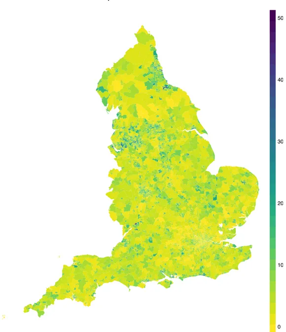
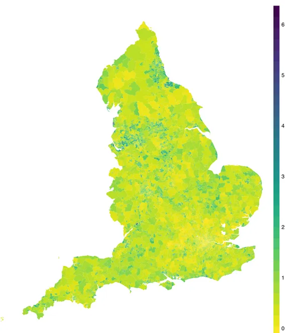
where t is a threshold value depending on the application (in this case we chose t = 0.9). The difference between the two methods is that in the former high risk areas are those where the risk increases for every level of the population, i.e. for those areas which are very sensible and those which are less sensible to the disease, while the latter considers only the mean level, which is a synthetic measure for the whole population but it may be subject to compensation. Figure 1.9 and 1.10 show the critical areas identified by quantile and mean regression. The similarity of the results of our method with those corresponding to a more traditional approach, as well as to previous analyses, reassures us that our method yields reasonable results. At the same time, the minor discrepancies between the two maps is also encouraging, as the two methods have different definitions of high risk; different results correspond in fact to different insights on the disease risk and the non-overlap between quantile-based exceedance probability-based methods testifies that there is information to be gained from our approach.

(32)

Hospitalization Counts 0 100 200 300 400 500

(33)

1.7. Quantile Regression for Poisson data 27

Standardized Morbidity Ratio

0 1 2 3 4 5 6

(34)

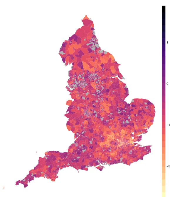
Exceedence Probability

−2 −1 0 1

Figure 1.9: Exceedence probability for Mean Relative Risk. In gray areas of High Risk.

(35)

1.7. Quantile Regression for Poisson data 29

Quantile Relative Risk

−2 −1 0 1

(36)

(37)

Chapter 2

Topological Tools for Data Analysis

2.1 The shape of fixed-scale data

As we are dealing with increasingly complex data, our need for characterizing them through a few, interpretable features has grown considerably. Topology has proven to be a useful tool in this quest for “insights on the data”, since it characterizes objects through their connectivity structure, i.e. connected components, loops and voids. In a statistical framework, this characterization yields relevant information: for example, connected components correspond to clusters (Chazal et al. 2013) while loops represent periodic structures (Perea and Harer 2015). At the crossroad between Computational Topology and Statistics, Topological Data Analysis (TDA from here onwards) is a new and expanding research area devoted to recovering the shape of the data focusing in particular on its topological structure (Carlsson 2009).

Although topology has always been considered a very abstract branch of mathematics, it has some properties that are extremely desirable in data analysis, such as:

• It does not depend on the coordinates of the data, but only on pairwise distances. In many applications, coordinates are not given to us or, even if they are, they have no meaning and they could be misleading.

• It is invariant with respect to a large class of deformations. Two object that can be deformed into one another without cutting or gluing are topologically equivalent, meaning that topological methods are flexible.

• It allows for a discrete representation of the objects we study. Most continuous objects can be approximated with a discrete but topologically equivalent object, for which it is easier to define algorithms.

2.1.1 Persistent Homology Groups - Intuition

The broad goal of TDA is to recover the topological structure (i.e. 0-dimensional topological features or connected components, 1-dimensional topological features or cycles and so on) of any arbitrary function of data f, by characterizing it in terms of some topological invariant, most often its Homology Groups, while also providing a measure of their importance.

The main advantage of this choice in terms of interpretability is that Homology Groups of dimension k represent k-dimensional connected structures: the Homology Group of

(38)

dimension 0 of a topological space X, H0(X) represents connected components of X, the

Homology Group of dimension 1, H1(X) represents loops (or cycles) of X, H2(X) represents

voids, and so on (we refer to Appendix B for a brief introduction of Homology Groups or to Hatcher (2002) for a more complete and rigorous treatment of the subject).

True Object −4 −2 0 2 4 − 4 − 2 0 2 4 −4 −2 0 2 4 − 4 − 2 0 2 4 Point Cloud −4 −2 0 2 4 − 4 − 2 0 2 4 Cover

Figure 2.1: From left to right: the true object we are trying to recover (X), the point–cloud data sampled on it (Xn) and the cover (dÁ).

In practice we most often do not observe the object we are interested in X directly, but a point–cloud Xn = {X1, . . . , Xn} sampled on it, which may not be explored using

Homology Groups directly. A point–cloud Xn, in fact, has a trivial topological structure

per se, as it is composed of as many connected components as there are observations and no higher dimensional features. Topological Invariants in the TDA framework are thus built from functions of Xn rather than on the point–cloud itself, using an extension of Homology,

Persistent Homology, which is the mathematical backbone of TDA (Edelsbrunner and Harer

2010).

Roughly speaking, Persistent Homology provides a characterization of the topological structure of any arbitrary function f by building a filtration on it (typically its sublevel or superlevel sets, fÁ and fÁ respectively). The link between Persistent Homology and the

“shape of the data” is that for some choice of f, sublevel (or respectively superlevel) set filtrations are topologically equivalent to the space data was sampled from, X.

Distance functions The most common choice for analysing the topological structure

of X is to investigate the Persistent Homology of the sublevel-set filtrations of a distance function. At each level Á, the Á-sublevel set of the distance d, dÁ, is defined as

dÁ =

n

€

i=1

B(Xi, Á),

where B(Xi, Á) = {x | dX(x, Xi) Æ Á} denotes a ball of radius Á and center Xi, and dXis an

arbitrary distance function. The metric d_X can be used to enforce some desired property, for example Chazal, Fasy, et al. (2014a) define a distance function, the Distance to Measure to

robustify the estimate. dÁ, usually called the cover of Xnis an approximation of the unknown

X that retains more topological information than the original point–cloud (Figure 2.1). The topology of dÁ coulf be investigated by computing its Homology Groups, however

(39)

2.1. The shape of fixed-scale data 33 estimate dÁ, with a different topological structure. As shown in Figure 2.2, when Á is small,

dÁis topologically equivalent to Xn: it consists of many connected components but no loops,

voids or other higher dimensional structures. Letting Á grow, balls in the cover start to intersect “giving birth” to more complex features, such as cycles. Gradually, increasing

Á causes connected components to merge and loops to be filled so that eventually dÁ is

topologically equivalent to a ball (or in other words, contractible) and again retains no information.

The key feature of encoding data into a filtration is that as Á grows, different sublevel-sets

dÁ1, dÁ2 are related, so that if a feature is present in both we can say that it remains alive in the interval [Á1, Á2]. Persistent Homology then allows to see how features appear and

disappear at different scales. Values Áb, Ád of Á corresponding to when two components are

connected for the first time (birth–step) and when they are connected to some other larger component (death–step) are the generators of a Persistent Homology Group.

In the statistical literature, dÁ is often known as the Devroye–Wise support estimator

(Devroye and Wise 1980). The consistency of the Devroye-Wise estimator justifies and motivates the use of the distance function: as dÁ is a consistent estimator of X, the topology

of dÁ is a reasonable approximation of the topology of X.

Kernel Density estimators The second way of linking levelset filtrations and the

topol-ogy of the support of the distribution generating the data, X, is that the super–levelsets of a density function p can be topologically equivalent to the support of the distribution itself as shown in B. T. Fasy et al. (2014). More formally, if the data are sampled from a distribution P supported on X, and if the density p of P is smooth and bounded away from 0, then there is an interval [÷, ”] such that the super–levelset pÁ = {x | p(x) Ø Á} is

homotopic (i.e. topologically equivalent) to X, for ÷ Æ Á Æ ”.

Since the true generating density p is most often unknown, it is typically approximated by a kernel density estimator p‚. A naive way to estimate the topology of X is hence to

compute topological invariants of the superlevel set of the kernel density estimatorp‚: ‚

pÁ= {x |p‚n(x) Ø Á}.

The superlevel setsp‚Á, with Á œ [0, maxp‚], form a decreasing filtration, which means that ‚

pÁµp‚” for all ” Æ Á. As in the case of distances, for each element in the filtration, i.e. for

each value Á, we obtain a different estimate p‚Á, whose topology can be characterized by its

Homology Groups. Since in practice it is not possible to determine the interval [÷, ”] in which the topology of p‚Á, is closest to that of X, we analyse the evolution of the topology in

the whole filtration. Once again, Persistent Homology allows to analyze how those Homology Groups change with Á. Persistent loops in p‚Á _{naturally represent circular structures in} _p_‚_,

Persistent Homology Groups of dimension 2 indicate holes inp‚and so on.

Far from being trivial, topological features of dimension 0, or connected components have also a relevant interpretation in terms of “bumps”. As can be seen from Figure 2.4, connected components in the filtrationp‚Á, are in fact local maxima of p‚; this is true for any

super–levelset filtration. When the filtration is defined in terms of sub–levelset instead, as in the case of the distance function, connected components represent local minima instead.