Forecasting Interest Rates Using Geostatistical Techniques

(1)

Econometrics 2015, 3, 733-760; doi:10.3390/econometrics3040733

econometrics

ISSN 2225-1146

www.mdpi.com/journal/econometrics

Article

Forecasting Interest Rates Using Geostatistical Techniques

Giuseppe Arbia 1_{and Michele Di Marcantonio}2,_*

1_{Department of Statistics, Catholic University of the Sacred Heart, Largo Francesco Vito,}

1-00168 Rome, Italy; E-Mail: giuseppe.arbia@rm.unicatt.it

2_{Department of Statistical Sciences, University of Rome “La Sapienza”, Viale Regina Elena,}

295-00161 Rome, Italy

* Author to whom correspondence should be addressed; E-Mail: michele.dimarcantonio@uniroma1.it;

Tel.: +39-333-384-1228.

Academic Editors: Fredj Jawadi, Tony S. Wirjanto, Marc S. Paolella and Nuttanan Wichitaksorn

Received: 31 July 2015 / Accepted: 29 October 2015 / Published: 9 November 2015

Abstract: Geostatistical spatial models are widely used in many applied fields to forecast

data observed on continuous three-dimensional surfaces. We propose to extend their use to finance and, in particular, to forecasting yield curves. We present the results of an empirical application where we apply the proposed method to forecast Euro Zero Rates (2003–2014) using the Ordinary Kriging method based on the anisotropic variogram. Furthermore, a comparison with other recent methods for forecasting yield curves is proposed. The results show that the model is characterized by good levels of predictions’ accuracy and it is competitive with the other forecasting models considered.

Keywords: term structure; yield curve; forecasting; geostatistics; variogram; Ordinary Kriging JEL classification: C3; C53; E43; E47

1. Introduction

The study of the evolution of interest rates through time represents one of the major challenges in quantitative finance literature. In recent years, with the growth of derivative contracts markets and with the evolution of portfolio and risk management techniques, studies on this issue have gained further importance from an empirical point of view. The increasing concern of policy makers, investors and market operators on accurate interest rate estimates and forecasts has further stressed the need of

(2)

defining models that are not only theoretically sound, but also usable in practice. In particular, according to Hunt et al. [1], they should be accurate, arbitrage-free, well-calibrated, realistic, transparent and characterized by observable parameters and by computationally acceptable times.

The two major objectives of the statistical analyses on interest rates are (i) the estimation of the term structure at a given point in time and (ii) the prediction of future rates. Despite few remarkable exceptions, in most cases the two objectives have been treated separately. With reference to the second objective, when forecasting interest rates, two dimensions are relevant: the moment of time of observations and the length of the term structure (the maturities). While the naïve approach forecasts the two dimensions separately, an obvious way of forecasting them jointly consists in the application of a multivariate time series modeling framework (Hamilton [2]). Section 2 contains a review of the most popular alternatives found in the literature.

This paper contributes to the existing literature by proposing a new, unified, approach for modeling interest rates as a joint function of their two fundamental dimensions (time and maturity) so as to achieve more accurate forecasts. Our approach thus deviates dramatically from the econometric strategies traditionally employed for modeling the term structure of interest rates as we rely on geostatistical methods and kriging forecasting techniques (Cressie [3]; Shabenberger and Gotway [4]). A pioneering study in financial literature based on geostatistical techniques can be found in Fernández-Avilés et al. [5], who cast the issue of international stock market comovements into a geostatistical framework. In our work, we explore further their potential applications in finance for the purposes of modeling and forecasting the term structure of interest rates. We build a fictitious three-dimensional space where the value of the interest rate is represented on the vertical axis, while the rate maturity and the reference time are reported on the two horizontal axes. On this surface, we interpolate an anisotropic variogram and adopt an ordinary kriging approach to forecast the out-of-sample values of the rates in different moments of time at different maturities.

Specifically, the interest rates considered in our empirical analyses are the Euro Zero Rates (EZR). EZR are determined as the zero-coupon yields which are implied in the term structure of Euro Swap Rates (ESR). Their relevance is due to the fact that the Euro interest rate swap market is one of the largest and most liquid financial markets in the world. In particular, the Euro swap curve has emerged as the preeminent benchmark yield curve in euro financial markets, against which even some government bonds are now often referenced (Remolona and Wooldridge [6]). In this sense, the EZR represent a valid proxy for measuring the risk free rate in the European context, comparable to US Treasury Bonds yields in US financial markets.

The paper is organized as follows. As said, Section 2 is devoted to a thorough literature review of the models currently used in interest rates modeling and forecasting. This section thus provides the necessary background to interpret the results of the methodology presented in Section 4. In Section 3, we briefly summarize some of the main concepts related to ordinary kriging forecast that we use in the rest of the paper. In Section 4, we present the data and the methodologies that we use for developing an empirical exercise where we apply the proposed model and other widely used prediction methods to forecast Euro Zero Rates on the basis of the data observed in the period 2003–2014. Section 5 presents the results of the empirical analysis, where we also test the accuracy of the proposed model both in absolute terms and compared with the alternative benchmark forecasting methods. Section 6 concludes.

(3)

Econometrics 2015, 3 735

2. Background on Estimating and Forecasting Models of Interest Rates

Interest rate term structure modeling is a widely studied issue in the financial literature and important theoretical advances have been reached so far in this area. The large interest of the scientific community on term structure modeling is witnessed by the huge number of alternative models proposed in the literature (for a review, see Brigo and Mercurio [7]; Subrahmanyam [8]). The large number and the heterogeneity of existing theories make it difficult to select a classification criteria; however, roughly speaking, two main approaches can be identified, namely: no-arbitrage models and equilibrium models.

The no-arbitrage approach aims at fitting the term structure under the assumption that no arbitrage opportunities should exist in the market; therefore, it plays an important role for pricing derivatives on interest rates. This hypothesis is used to derive the prices of all contingent claims making assumptions on the evolution of one or more interest rates. The no-arbitrage approach in interest rate theory is grounded on the general theory of arbitrage based in turn on the Black-Scholes equation (Black and Scholes [9]). A prominent contribution in this vein includes the work of Merton [10], Brennan and Schwartz [11], Ho and Lee [12], Hull and White [13] and Heath et al. [14] amongst the many others. Within the general framework proposed by Heath et al. [14], further extensions have been proposed by Brace et al. [15], Brace and Musiela [16], Goldys et al. [17], Musiela [18] and Musiela and Rutkowski [19]. An in-depth study of models for the evaluation of contingent claims subject to default risk can be found in Duffie and Singleton [20]. With reference to LIBOR and swap market models, a pricing and hedging theory was proposed by Jamshidian [21], while de Jong et al. [22] develop a multi-factor econometric model of the term structure of interest-rate swap yields which accommodates for the possibility of counterparty default.

In contrast to this line of research, the equilibrium approach is focused on the derivation of the interest rates and the price of all contingent claims, from a description of the underlying economy and from a set of assumptions on the stochastic evolution of one or more exogenous variables in the economy and on the preferences of a representative investor (Longstaff and Schwartz [23]). The equilibrium approach was pioneered by Cox et al. [24–26], whose model (together with the mean-reverting processes proposed by Vasicek [27]), constitutes the major reference within the literature on (spot) short interest rate dynamics. Black and Karasinski [28] generalized the exponential Vasicek model, defining a one-factor lognormal model for short term interest rate that allows the target rate, long term mean and local volatility to vary through time. Alternative models for the stochastic process of the (spot) short term interest rate have been introduced by Dothan [29] and Hull and White [30]. For an empirical comparison of the main short-term interest rate models see Broze et al. [31] and Chan et al. [32], while a review of diffusion processes of interest rates can be found in Monsalve-Cobis et al. [33].

Several term structure affine models have been proposed in the academic literature. Duffee [34] examined the forecasting ability of standard class of affine models showing that the random walks assumption produces better forecasts. Along the same lines Duffie and Kan [35] defined a multifactor affine model of the term structure of interest rates. Within the area of multifactor models of interest rates it must be noticed that, due to practical restrictions connected with the computational complexity, the number of factors is usually limited to a maximum of two, although some three factor models may be found in literature. In this sense, Brennan and Schwartz [11] consider as factors the short and the

(4)

long term interest rate, while Schaefer and Schwartz [36] use, instead, the short term rate and the spread between the long and the short term rate. A recent series of theoretical and empirical investigations on term structure affine models can be found in Jakas [37–41].

With reference to the analysis of forward rates, an important contribution to modeling the term structure is represented by the Nelson and Siegel [42] model, also widely used in many empirical applications. Svensson [43] proposed the inclusion of an additional term in the Nelson and Siegel [42] model to increase flexibility and improve the fit of the term structure model. By making a comparison with Nelson and Siegel [42] model, in a recent study Gimeno and Nave [44] demonstrated that using an alternative optimization methodology based on genetic algorithms produces better estimates as well as greater stability of the parameters that determine the fit.

Conversely, despite their growing practical importance, relatively little work has been done on forecasting models of the yield curve. As evidenced by Diebold and Li [45], research (or studies) on arbitrage-free term structure have little to say about dynamics of forecasting, as it focuses on fitting the term structure at a given moment of time. In fact, affine equilibrium models are focused on the dynamics driven by the short rate and they are potentially linked to forecasting; however, since most studies develop in-sample fit of the term structure (Dai and Singleton [46]; de Jong [47]), they are not suitable for out-of-sample predictions.

One of the early contributions in interest rates forecasting is the work of Fama and Bliss [48]. Their work is a pioneering study on the information in forward rates about future interest rates, but still has the limitation of estimating independent regressions for each yield, ignoring the empirical evidence that the yields on bonds of different maturities are highly correlated. In order to overcome these limitations, dynamic versions of the term structure models have been proposed afterwards. Among these, a prominent contribution is the model developed by Diebold and Li [45] (based on the Nelson and Siegel [42]) model, who use an autoregressive model for each factor in order to develop predictions that are consistent for each maturity of the term structure. Galvao and Costa [49] have developed further their approach by considering also the dynamic correlations between the slope, the level and the curvature, by using vector autoregressive models. In a recent work, Chen and Niu [50] have improved the dynamic model of Diebold and Li [45] by defining an adaptive model to detect parameters’ changes and forecast the yield curve. Similarly, Xiang and Zhu [51] have defined a dynamic version of the Nelson-Siegel model that is subject to regime shifts by introducing the reversible jump Markov chain Monte Carlo method, which allows jumps between the one-, two- and three-regime models.

Finally, a further alternative approach in this field is the Cochrane and Piazzesi [52] forward curve regression. Part of the literature supports the thesis that forward rates differ from expected future yields by maturity-dependent constants and/or time-varying expected excess return (for a review see Duffee [53]). However, a relevant part of scholars in this field considers the forward rate as a rational forecast of the (spot) zero rate with the same maturity to be observed in a future moment of time (Fama and Bliss [48]; Galvao and Costa [49]).

The high number of models proposed so far by researchers evidences that the issue of estimating and forecasting the term structure of interest rates is still being explored, hence the debate for identifying the best models for in-sample and out-of-sample predictions is still open. However, there is a wide consensus among scholars and financial institutions on the primary role of the Nelson-Siegel [42]

(5)

model and its subsequent versions (among which Svensson [43], Diebold and Li [45], Chen and Niu [50]) for estimating and forecasting the term structure of interest rates. This is confirmed by the number of alternative and/or subsequent extensions of the original Nelson-Siegel model which have been proposed to date, mostly with the objective of defining a dynamic version for out-of-sample predictions. Furthermore, the practical relevance of the Nelson-Siegel framework is witnessed by the fact that some of the main financial institutions as the International Monetary Fund (Gasha et al. [54]), the European Central Bank and the Federal Reserve (Moench [55], Bolotnyy [56]) rely on it for their studies and activities. Nyholm and Vidova-Koleva [57] confirm that the best out-of-sample performance is generated by three-factor affine models and the dynamic Nelson-Siegel model variants, while quadratic models provide the best in-sample fit.

3. Geostatistical Methods: A Brief Overview

Spatial statistical methods constitute a relatively new area of research that emerged in the last decades with application in very different scientific fields (Cressie [3]; Matheron [58]; Ripley [59]). Traditionally, applications can be found in many applied fields in order to forecast data observed on continuous three-dimensional surfaces, as geology, hydrology, meteorology, oceanography, geography, environmental studies, soil sciences, agriculture and epidemiology to name only few. Spatial statistical applications in finance are conversely very rare with few remarkable examples represented by the contribution of Kennedy [60] on a two-dimensional modeling of financial events, and the work of Bauewens and Hautsch [61,62], Hautsch [63,64] and Resnick [65] on high-frequency financial duration data modeled as point patterns (Boots and Getis [66]; Diggle [67]). Adding to the meager literature in this area, in the present paper we propose the use of geostatistical methods to forecast interest rates.

In order to introduce the geostatistical approach, let us first define a random field Z ( ): ∈ ⊂ ℜ as a collection of random variables ordered with respect to two continuous coordinates ≡ ( , ). We assume the random field to have a mean ( ) = and a finite variance ( ) = . For modeling convenience, we often assume the field to be Gaussian (that is ( ) ≈ ( ; ), with the variance-covariance matrix) and intrinsically stationary, that is satisfying the conditions that

( + ℎ) − ( ) = 0 and:

( + ℎ) − ( ) = Var ( + ℎ) − ( ) = 2 (ℎ) (1) The function (ℎ) in (1) is called the semivariogram of the spatial random field and h is the distance between two points on the surface. If the semivariogram depends only on h and not on the direction, it is said to be isotropic (as opposed to anisotropic). Theoretical isotropic semivariograms can assume different specifications like, e.g., Power, Bessel, Linear, Gaussian, Spherical, Exponential and others (see Shabenberger and Gotway [4]).

One of the simplest models is the Gaussian semivariogram defined as: (ℎ) = + 1 − exp(− ℎ ) ifℎ ≥ 0

0 otherwise (2)

which is characterized by three parameters to be empirically estimated termed, respectively, the nugget ( ), the sill ( ) and the range ( ).

(6)

Other models often used in the literature are the Exponential semivariogram, defined as: (ℎ) = + 1 − exp(− ℎ) ifℎ ≥ 0

0 otherwise (3)

the Power semivariogram, defined as:

(ℎ) = + ℎ( ⁄ ) ifℎ ≥ 0 and > 1/2

0 otherwise (4) and the Bessel semivariogram, defined as:

(ℎ) = + 1 − ℎ ( ℎ) ifℎ ≥ 0

0 otherwise (5)

where Kv(·) is the Bessel function of the first kind of order v. In order to simplify notations, the lag distance

is always indicated as h, as it is clear that it is a scalar or a vector depending on the reference model.

From the above definitions, the problem of prediction in geostatistics can be summarized as follows: given the random field Z observed in n sites, predict its value in an unobserved site, say s0. The kriging

solution to this problem (see Krige [68]) can be obtained by introducing a linear predictor for ( ), call it ( ), defined as:

( ) = ( ) + (6)

and deriving a set of optimal weights li minimizing the mean squared error ( ) − (∑ ( ) +

) . Under the constraint of a constant mean (which implies ∑ = 1) the optimization problem can be expressed as:

( ) − ( ) = ( ) = min (7)

having set = 1 and = − ∀ ≠ 1. It can be shown that, for each theoretical semivariogram the optimal weights can be expressed as an analytical function of the semivariogram γ. As a consequence, under the previous definitions, the ordinary kriging strategy consists in fitting a theoretical semivariogram to the empirical data, use the fitted semivariogram to derive the optimal weights and, finally, use them to forecast the data on the surface using Equation (6).

In the present paper, we adopted an ordinary kriging approach instead of a universal kriging for the sake of comparison with the other competing models. In fact, the LARX model used for updating the parameters of the DNS benchmarking model employs only the inflation rate as exogenous variable and there is no way of using this variable in a universal kriging approach; this is because we can only observe its evolution through time, and not also through the maturity axis. In this respect, our results reinforce the power of the proposed approach, which achieves very accurate forecasts compared with the DNS model even if it is a purely autopredictive model that does not use any regressors.

In the next section, we will exploit this analytical framework to forecast interest rates along the time and maturity dimension. To implement our procedure we build up a fictitious three-dimensional space where the value _. of a given zero rate with maturity m observed at time t is represented on the vertical axis z, while m and t are reported on the horizontal axes x and y, respectively. We assume this to represent a three-dimensional surface with some unobservable data points (the future observations) that can be conveniently forecasted using the kriging strategy described above. The proposed strategy will be illustrated in the following section through an empirical application.

(7)

4. An empirical Application: Forecasting Euro Zero Rates 4.1. Data Description

In order to test on empirical data the accuracy of the kriging forecasting model proposed in the previous section, we consider an interest rate characterized by a plurality of maturities and with sufficiently long historical data. As said, considering their importance in the European context and the relative length of their time series, we selected the Euro Zero Rates (EZR). Specifically, in each time period, EZR represent the Euribor 12-months rate for the maturity one year, while they were derived by bootstrapping the Euro Swap Rates (ESR) for maturities from 2 to 50 years. For a description of swap contracts, swap rates and bootstrapping procedures see Hull [69].

In order to assess the accuracy of our kriging forecasting model we compared its performances with the results of two other prediction methods: an extended version of the dynamic Nelson-Siegel (DNS) model, as better described in Section 4.3, and forward rates. With reference to the latter, at each moment of time t (the end of each year of the selected historical period) we considered the forward rates implicit in the EZR curve at the same date t (the Euro Forward Rates, call them “EFR”), for the same maturities m and for a given time horizon h. Thus, ESR were used to derive the EZR for maturities higher than one year, while EFR were used to compare the accuracy of our spatial forecasting model with respect to the market expectations of future EZR. Hereinafter, we will refer to

. as the value of the EZR with maturity m observed at time t, while with the symbol , , we

indicate the value of the EFR with maturity m, observed at time t and with a time horizon h. Table 1 summarizes the common features and the specific characteristics of the EZR, ESR and EFR considered in our work.

The observational period ranges between 1 January 2003 and 30 June 2014. In particular, the historical data used to estimate the empirical variogram ranges from the 1 January 2003 to 31 December 2013, while the last six months (from 1 January 2014 to 30 June 2014) have been used only as out-of-sample data to assess the accuracy of the forecasting procedure. The empirical data were collected on the 1 July 2014 on a daily basis, excluding non-trading days: as a consequence, for each maturity, we considered about 256 observations per year. On each day we record the closing value, as reported by the Bloomberg financial database. Table 2 illustrates some summary statistics of the daily observations of EZR collected for each maturity, while Table 3 shows the values of EFR (expressed as percentage points) with a time horizons h = 3, 6 and 12 months that are implicit in the EZR curve at the end of each year of the period, for the maturities of 10, 20 and 30 years.

Figure 1 shows the surface of EZR sample data, obtained through a linear interpolation of the _. values expressed as percentages. Both axes are expressed in years. The graph shows clearly a decreasing trend in the 10 years considered from 2003 to 2013 along the t axis associated with an increasing trend of the rates moving from short maturities to long term maturities along the m axis.

(8)

Table 1. Main features of the interest rates considered. Common Features

Maturities m (years) 1, 2, 3, 4, 5, 6, 7, 8, 9, 10, 11, 12, 15, 20, 25, 30, 40 and 50

Period From 1 January 2003 to 30 June 2014

Reference curve Euro (ID: S45)

Data source Bloomberg

Specific Features

Type of rate Swap Zero Forward (Zero)

Name EUR Swap Annual EUR Zero Rate EUR Forward (Zero) Rate

Bloomberg ticker EUSAm Curncy S0045Z mY BLC2 Curncy -

Symbol ESR EZR EFR

Time horizon h (months) - - 3, 6 and 12

Day count Fixed 30U/360

Determined by bootstrapping the EUR Swap Annual curve for m ≥ 2,

while for m = 1 it was considered the Euribor 12 months ACT/360

(ticker: EUR012M Index).

Determined on the basis of the EUR Swap Annual bootstrapped

curve (rate type “Zc”, side “Mid”) using the “BCurveFwd”

Bloomberg function. Floating ACT/360 Payment frequency Fixed Annual Floating Semi-annual Floating

Index Euribor 6 months

Index ticker EUR006M Index

Reset frequency Semi-annual

Note: Bloomberg tickers are specific for each maturity; therefore, given a maturity of (e.g.,) m = 7 years, the notation (e.g.,) “EUSAm Curncy” indicates that the Bloomberg ticker is “EUSA7 Currency”. The selected maturities, the reference period and the source of data are the same for each type of rate, while the technical characteristics are specific for Euro Swap Rates (ESR), Euro Zero Rates (EZR) and Euro Forward Rates (EFR).

(9)

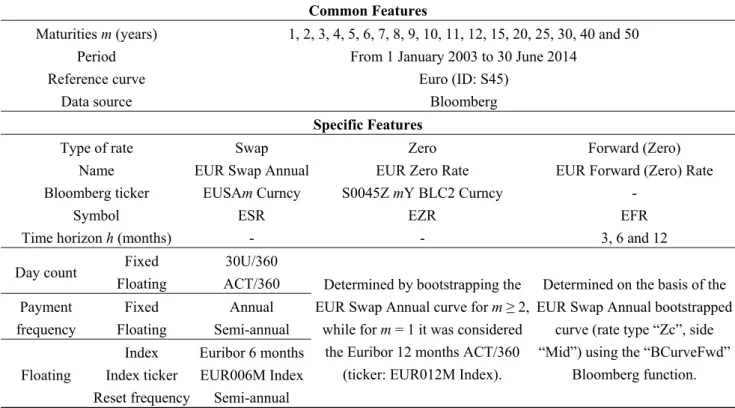
Table 2. Descriptive statistics of Euro Zero Rates (EZR). Maturity m (Years) 1 2 3 4 5 6 7 8 9 10 11 12 15 20 25 30 40 50 2003 2.33 2.64 2.96 3.26 3.51 3.73 3.92 4.09 4.23 4.35 4.46 4.56 4.79 5.04 5.14 5.15 5.09 5.00 2004 2.27 2.64 2.97 3.25 3.49 3.70 3.88 4.04 4.18 4.29 4.39 4.48 4.70 4.94 5.04 5.07 5.07 5.03 2005 2.33 2.54 2.71 2.85 2.99 3.12 3.24 3.35 3.45 3.54 3.62 3.69 3.86 4.03 4.11 4.13 4.14 4.12 2006 3.44 3.62 3.69 3.75 3.80 3.84 3.89 3.93 3.98 4.02 4.06 4.10 4.19 4.28 4.31 4.30 4.25 4.19 2007 4.45 4.44 4.43 4.43 4.45 4.46 4.48 4.51 4.54 4.57 4.60 4.63 4.70 4.75 4.74 4.70 4.60 4.49 2008 4.83 4.32 4.29 4.30 4.32 4.35 4.40 4.45 4.50 4.55 4.60 4.65 4.74 4.75 4.64 4.54 4.37 4.23 2009 1.61 1.88 2.28 2.59 2.85 3.07 3.25 3.40 3.53 3.65 3.75 3.85 4.07 4.19 4.05 3.89 3.57 3.43 2010 1.35 1.47 1.75 2.02 2.27 2.50 2.69 2.86 3.00 3.12 3.23 3.32 3.53 3.62 3.54 3.37 3.14 3.06 2011 2.01 1.85 2.06 2.28 2.50 2.67 2.83 2.95 3.06 3.16 3.25 3.34 3.52 3.57 3.47 3.34 3.20 3.18 2012 1.11 0.78 0.88 1.04 1.24 1.43 1.61 1.76 1.89 2.01 2.12 2.21 2.40 2.47 2.44 2.41 2.46 2.53 2013 0.54 0.52 0.68 0.89 1.10 1.30 1.49 1.66 1.82 1.96 2.09 2.20 2.44 2.59 2.62 2.61 2.66 2.73 2014 0.57 0.44 0.57 0.75 0.95 1.15 1.34 1.52 1.69 1.83 1.96 2.08 2.33 2.52 2.56 2.56 2.57 2.57 Observations 2944 2944 2944 2944 2944 2944 2944 2944 2944 2944 2944 2944 2944 2944 2944 2944 2944 2944 Mean 2.31 2.34 2.52 2.70 2.87 3.02 3.16 3.29 3.40 3.49 3.58 3.66 3.84 3.96 3.95 3.90 3.81 3.76 St. deviation 1.34 1.32 1.26 1.21 1.15 1.10 1.06 1.02 1.00 0.97 0.95 0.93 0.91 0.92 0.94 0.96 0.94 0.90 Minimum 0.47 0.31 0.39 0.50 0.65 0.82 1.00 1.17 1.33 1.47 1.60 1.71 1.89 1.88 1.85 1.81 1.83 1.85 Maximum 5.53 5.48 5.40 5.27 5.19 5.14 5.10 5.08 5.07 5.09 5.10 5.12 5.15 5.28 5.38 5.40 5.43 5.37

This table shows the one-year means of the daily values of Euro Zero Rates (%) observed within each year of the reference period (1 January 2003–30 June 2014) and some descriptive statistics related to the whole dataset for each examined maturity.

(10)

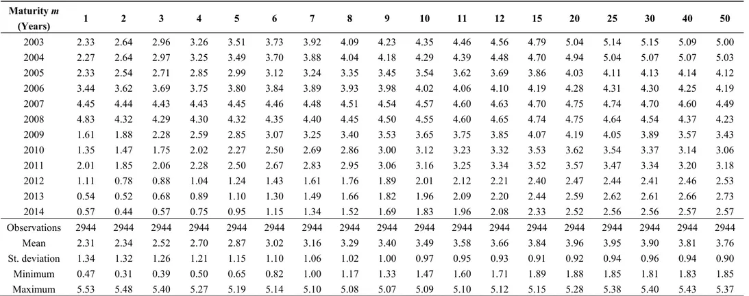
Table 3. Descriptive statistics of Euro Forward Rates (EFR).

Date t Year 2003 2004 2005 2006 2007 2008 2009 2010 2011 2012 2013 Day/Month 29/12 28/12 31/12 31/12 31/12 30/12 29/12 31/12 31/12 31/12 31/12

Time horizon h Maturity m = 10 (years)

3 month 4.54 3.90 3.51 4.22 4.75 3.83 3.77 3.46 2.46 1.66 2.29

6 months 4.62 3.97 3.54 4.23 4.76 3.89 3.87 3.55 2.51 1.73 2.37

12 months 4.78 4.08 3.59 4.24 4.80 4.01 4.04 3.70 2.63 1.86 2.53

3 month 5.07 4.45 3.83 4.35 4.98 3.92 4.25 3.85 2.75 2.28 2.86

6 months 5.12 4.48 3.84 4.36 4.98 3.92 4.28 3.88 2.76 2.31 2.90

12 months 5.19 4.54 3.87 4.36 4.99 3.94 4.35 3.93 2.80 2.36 2.96

3 month 5.18 4.56 3.86 4.29 4.90 3.45 3.98 3.49 2.56 2.33 2.83

6 months 5.21 4.58 3.86 4.29 4.90 3.44 4.00 3.50 2.56 2.35 2.85

12 months 5.25 4.62 3.88 4.29 4.90 3.44 4.03 3.51 2.58 2.39 2.88

This table reports the values of Euro Forward Rates (%) with a time horizons h = 3, 6 and 12 months implicit in the Euro Zero Rates curve at the end of each year t of the period examined, for a maturity of 10, 20 and 30 years.

Figure 1. Three-dimensional representation of Euro Zero Rates sample data (see Table 1),

obtained through a linear interpolation of the , values expressed as percentages. The

value _, of the EZR with maturity m observed at time t is represented on the vertical axis z, while m and t are reported on the horizontal axes x and y, respectively. The surface is represented using different tones for each range of 100 basis points (from 0 to 600) of _, .

4.2. The Ordinary Kriging Model

In order to forecast the term structure of EZR for all the maturities and all time period, we adopt a three-steps procedure. At a first step, we calculate the empirical anisotropic variogram of the sample observations by choosing a cutoff parameter of 12 months. This value represents the limiting spatial distance to include pairs of observations in the semivariance estimates: outside this threshold pairs of

(11)

observations are not considered. In a second step, we calibrate the best-fitting model among four different variograms, namely: Bessel, Exponential, Gaussian and Power (see Section 3) 1_{. In all cases,}

the nugget is set equal to zero, the sill and the range are fitted empirically for each model and the geometric anisotropy parameters are determined through the Covariance Tensor Identity (CTI) method 2_.

Finally, in the third step, in order to obtain out-of-sample forecasts of the values of the EZR, we interpolate the data using the ordinary kriging based on the variogram selected in step 2. In all cases, a time horizon of 12 months is considered.

In order to test the accuracy of the proposed model, we forecast the values of the last working day of December of each year (2003 to 2013), for a total of 11 reference dates (see Table 3). In order to assess whether the use of a wider set of observations significantly improves the accuracy, the procedure is replicated considering also different lengths of time: one year (d = 1), three years (d = 3) and all the available data from 1 January 2003 (d = max) (for a study on the short and long memory effects on interest rate processes, see, e.g., Baillie [70] and Duan and Jacobs [71]). All in all, we consider 29 theoretical anisotropic variograms fitted to the empirical data on a weekly basis through which we determine 31 kriging forecasts. (Two repetitions occurred when d = max in 2003 and 2005, because they coincide in different models). Daily instead of weekly data are considered for d = 1, in order to consider a sufficient number of historical observations. For sake of brevity hereinafter the proposed spatial model is indicated as the “OK” (Ordinary Kriging) model.

4.3. The Extended Dynamic Nelson-Siegel Model

The dynamic Nelson-Siegel model, proposed by Diebold and Li [45], is a dynamically-evolving version of the well-known Nelson and Siegel [42] model. This model does not directly forecast the yield curve, as it follows a factor approach where, in primis, autoregressive models are used to forecast the factors and, then, the Nelson-Siegel model is applied to forecast the yield curve on the basis of the factors’ predicted values. The factors of the Nelson-Siegel model are interpreted as the level, the slope and the curvature of the term structure. As demonstrated by Diebold and Li [45], the DNS model shows good levels of forecasting ability compared with other statistical methods and it has become a commonly used tool for the prediction of the yield curve. The formulation of the yield curve in the Nelson and Siegel [41] framework is specified in Equation (8).

, = +

1 −

+ 1 − − + , (8)

where , is the interest rate with maturity m at time t and , ≈ (0, ). The parameter λ governs

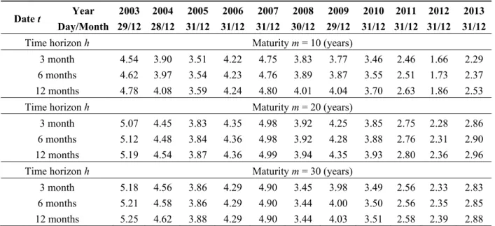
the exponential decay rate of the curve loadings for the slope and the curvature factors. In particular, small (large) values of λ produce slow (fast) decay and can better fit the curve at long (short) maturities. In this work, the value of λ was set equal to 0.3189, which is the simple arithmetic average of the λ values obtained by fitting the Nelson-Siegel model for each date of the period between 1 January 2003 and 30 June 2014, on a weekly basis 3_{. Factor loadings on the yield curve are displayed in Figure 2.}

1_{All computations were performed using the software R.}

2_{Using the “EstimateAnisotropy” function of the software R (package “Intamap”).}

(12)

Figure 2. Nelson-Siegel factor loadings (λ = 0.3189).

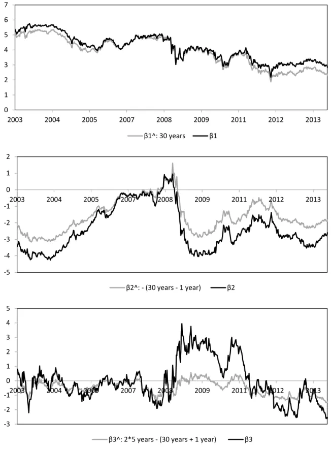
The loadings of β are equal to 1 for all maturities, therefore that the higher the factor, the higher the level of the whole yield curve. Empirically it can be proxied by the long-term yield of 30 years. The loadings of β start from 1 at the instantaneous spot rate (m = 0) and decay towards zero as maturities increase. The value of β is negative in most of the cases, indicating that the term structure is usually upward-sloping. The factor β is highly correlated with the negative spread of the yield curve, i.e., the difference between the short-term and long-term yields; in this work we considered the difference between r and r , hence − r − r . The loadings of the curvature factor β reach a maximum around the maturities of medium duration and decays towards zero as maturities increase. A positive value of β indicates that the yield curve is concave with a hump, while a negative value means that the yield curve is convex with an inverted hump (Chen and Niu [50]). Empirically, β can be approximated by twice the medium yield minus the sum of the short- and long-term yields, e.g., 2r − r + r . Figure 3 shows the time evolution of the three factors (black lines) and their respective empirical proxies (grey lines). The correlations between the three factors and their proxies are equal to 0.979, 0.977 and 0.867, respectively.

0 0.2 0.4 0.6 0.8 1 1.2 0 10 20 30 40 50 Factor loading Maturity (years) Level Slope Curvature

(13)

Figure 3. Time evolution of Nelson-Siegel factors for Euro Swap Zero Rates.

The time evolution of the factors , and —the level, the slope and the curvature, respectively—is determined through univariate autoregressive AR(1) processes for each single factor or with a multivariate autoregressive VAR(1) model for the three factors simultaneously. Following Chen and Niu [50], we focus on the AR(1) model, motivated by its simplicity, parsimony and good

0 1 2 3 4 5 6 7 2003 2004 2005 2007 2008 2009 2011 2012 2013 β1^: 30 years β1 -5 -4 -3 -2 -1 0 1 2 2003 2004 2005 2007 2008 2009 2011 2012 2013 β2^: - (30 years - 1 year) β2 -3 -2 -1 0 1 2 3 4 5 2003 2004 2005 2007 2008 2009 2011 2012 2013

(14)

level of out-of-sample prediction accuracy, and we consider exogenous variables, i.e., a LARX(1) model, for each Nelson-Siegel factor. The LARX(1) model is defined through a time varying parameter , where = ( , , , ) (9).

= + + + (9)

where the common exogenous variable is the inflation rate and ≈ (0, ). Once identified the reference sample of observations, the parameter can be estimated through the ordinary least squares (OLS) method.

A further refinement of the Nelson and Siegel [42] model was proposed by Chen and Niu [50], starting from the dynamic Nelson-Siegel model. In particular, they define an adaptive version of the model that is able to adaptively detect parameter changes (the ADNS model). Given a reference point of time s, all available past information are taken but only a subsample that includes all the observations that can be well represented by a local stationary model with approximately constant parameters is considered. The procedure allows to determine the local maximum likelihood estimator

on the basis of the subsample of observations referred to the optimal period − ; .

However, since our objective is comparing the prediction ability of the proposed OK model with the accuracy of other forecasting methods, the same historical observations shall be considered to apply all the models at each forecasting date. Therefore, in this work, the optimization procedure of the ADNS model was not applied. As said, we focus on the DNS model, considering the extension proposed by Chen and Niu [50] where a LARX(1) model with the inflation rate as exogenous variable is used for forecasting the Nelson-Siegel factors. In particular, since we focused on Euro Swap Rates, we consider the annual growth rate of the Eurostat “MUICP All Items” (ECCPEMUY) monthly index as a measure of the inflation rate in the Eurozone, linearly interpolated in order to obtain daily values.

4.4. Measures of Prediction Accuracy

In order to test the accuracy of forecasts, for each examined model (OK and DNS) we calculate statistics based on the root mean squared error (RMSE), defined as the square root of the mean squared error. We considered the RMSE as it represents a standard measure in the financial literature for measuring and comparing the accuracy of interest rates prediction models (Diebold and Li [45], Chen and Niu [50], Christensen et al. [72], Yu and Zivot [73], Coroneo et al. [74]).

In particular, in order to refine our comparative analysis, we consider alternative versions of the RMSE, based on statistics other than the mean, that are the minimum value, the maximum value and the quartiles of the models’ squared errors. Therefore, for each statistic S:{Minimum; 1st Quartile;

Median; 3rd Quartile; Maximum} of the squared errors, we calculated the “RSSE”, where the mean

statistic (“M”) considered in the standard RMSE formula is substituted by each selected statistic S, in Equation (10):

̂ _, _, = S ̂ _, _, − _, (10)

where the notation “model” indicates either the OK or the DNS model and S[·] is the formula of each statistic S of the squared errors. Therefore, we determine and , respectively. In

(15)

Equation (10), _, represents the value of the EZR at time t + h with maturity m and ̂ _, _, is the value predicted at time t through the OK or the DNS model using a historical dataset of d years.

Furthermore, for the sake of comparison, we calculate the RSSE of EFR predictions as follows:

, , = S , , − , (11)

where, in addition to the previous symbols, _{, ,} is the EFR with maturity m, obtained at time t and time horizon h. The RSSE of EFR is used as a comparative market benchmark for individually assessing the accuracy of both the OK and the DNS models.

5. Empirical Results

5.1. The Ordinary Kriging Model

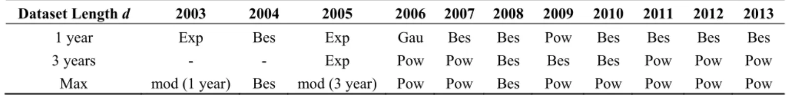
For each of the 31 combinations [t; d] described in Section 4.2, we selected the best-fitting variograms (Bessel, Exponential, Gaussian and Power) to the empirical variogram. Table 4 summarizes the selection results.

Table 4. Theoretical anisotropic variogram models.

Dataset Length d 2003 2004 2005 2006 2007 2008 2009 2010 2011 2012 2013

1 year Exp Bes Exp Gau Bes Bes Pow Bes Bes Bes Bes

3 years - - Exp Pow Pow Bes Bes Bes Pow Pow Pow

Max mod (1 year) Bes mod (3 year) Pow Pow Bes Pow Pow Pow Pow Pow

This table reports the theoretical anisotropic variogram models which best fit the empirical variogram for each combination of reference year t and dataset length d of the Euro Zero Rates’ time series. These theoretical anisotropic variogram models are used for applying the Ordinary Kriging prediction method. The abbreviations have the following meaning: “Bes” = Bessel; “Exp” = Exponential; “Gau” = Gaussian; “Pow” = Power. The cells with “-” indicate that the historical dataset available at the reference rate is not enough for the requested dataset amplitude, while the cells with “mod(x)” indicate that the selected model coincides with the one fitted for d = x at the same reference date.

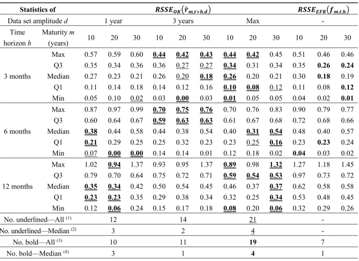
On the basis of the selected variogram models shown in Table 4, for each combination [t; d] we apply the OK method in order to predict the term structure of EZR for all the dates included in the period from 31 December of t to 31 December of the following year (t + 1). To facilitate the presentation of the results, we limit the evaluation of the accuracy of the method to the EZR with maturity 10, 20 and 30 years. For the same reason, we only consider the forecasts with time horizon 3 months (at 31/03/t + 1) 4_{, 6 months (at 30/06/t + 1) and 12 months (at 31/12/t + 1) ahead from t. The}

results are thus presented as a function of three elements: the maturity m (10, 20 or 30 years), the forecasts’ time horizon h (3, 6 or 12 months) and the information set used d (1, 3 years or max). Table 5 shows the results of the analyses expressed in terms of the ̂ , , and , , .

As it was reasonable to expect, forecasts are characterized by higher median errors and a higher level of uncertainty when a greater forecasts’ time horizon is considered. In particular, using the

(16)

max-length dataset, the median ̂ , , is between 0.20 and 0.26 for predictions of three

months ahead while it rises between 0.31 and 0.54 for 6 and 12 months ahead-predictions.

Table 5. Prediction accuracy of the Ordinary Kriging (OK) model and the Euro Forward

Rates (EFR) forecasting method (overall analysis).

Statistics of , , , ,

Data set amplitude d 1 year 3 years Max -

Time horizon h Maturity m (years) 10 20 30 10 20 30 10 20 30 10 20 30 3 months Max 0.57 0.59 0.60 0.44 0.42 0.43 0.44 0.42 0.45 0.51 0.46 0.46 Q3 0.35 0.34 0.36 0.36 0.27 0.27 0.34 0.31 0.34 0.35 0.26 0.24 Median 0.27 0.23 0.21 0.26 0.20 0.18 0.26 0.20 0.21 0.30 0.18 0.19 Q1 0.11 0.14 0.18 0.14 0.12 0.16 0.10 0.08 0.12 0.11 0.08 0.12 Min 0.05 0.10 0.02 0.03 0.00 0.03 0.01 0.05 0.05 0.04 0.02 0.01 6 months Max 0.87 0.97 0.99 0.70 0.75 0.76 0.70 0.76 0.83 0.90 0.79 0.77 Q3 0.60 0.64 0.67 0.59 0.63 0.63 0.61 0.67 0.68 0.72 0.68 0.66 Median 0.38 0.44 0.58 0.44 0.38 0.54 0.40 0.31 0.54 0.48 0.40 0.57 Q1 0.21 0.29 0.25 0.25 0.32 0.23 0.23 0.25 0.16 0.23 0.23 0.24 Min 0.07 0.00 0.00 0.14 0.14 0.01 0.12 0.18 0.02 0.04 0.03 0.02 12 months Max 1.02 0.94 1.37 0.93 0.95 1.37 0.89 0.98 1.32 1.27 1.18 1.45 Q3 0.79 0.70 0.64 0.75 0.72 0.71 0.59 0.54 0.53 0.97 0.73 0.72 Median 0.35 0.34 0.42 0.50 0.54 0.45 0.46 0.37 0.37 0.62 0.58 0.58 Q1 0.23 0.23 0.35 0.29 0.38 0.34 0.32 0.25 0.34 0.53 0.48 0.45 Min 0.12 0.06 0.24 0.15 0.17 0.18 0.08 0.20 0.06 0.32 0.29 0.26 No. underlined—All (1)₁₂ ₁₄ ₂₁ _- No. underlined—Median (2)₃ ₂ ₄ _- No. bold—All (3)₁₀ ₁₁ ₁₉ ₇ No. bold—Median (4)₃ ₁ ₄ ₁

(1)_{Number of underlined statistics (total = 45, plus eventual repetitions for d = max);}

(2)_{Number of underlined median values (total = 9, plus eventual repetitions for d = max);}

(3)_{Number of statistics in bold (total = 45, plus eventual repetitions for d = max);}

(4)_{Number of median values in bold (total = 9, plus eventual repetitions for d = max).}

The statistics shown in this table are presented in terms of root square of each statistic S:{Minimum; 1st Quartile;

Median; 3rd Quartile; Maximum} of the models’ squared errors observed at the reference dates (t), defined,

respectively, as ̂ , , and , , . RSSEs’ statistics are presented for each

combination of maturity (m = 10, 20 and 30 years), time horizon h (3, 6 and 12 months) and dataset length

d (1, 3 years and max) considered. Underlined statistics have the lowest value among the first three columns d = 1, d = 3 and d = max (to identify the best d for applying the OK model), while boldface statistics have the

lowest value among all the four columns (to identify the best prediction method between the OK model and the EFR).

Table 5 shows that, in most cases, the best forecasts are achieved by using the max-length dataset. In particular, when d = max, the kriging forecast outperforms the forward rate method—in terms of lower RSSE statistics (median statistic)—in 33 (7) cases out of 45 (9). The OK method turns out to be even more accurate than the forward rates method as the time horizon h increases (reaching the

(17)

variogram cutoff); in particular, for 12 months ahead forecasts the OK model outperforms the forward rate method—in terms of lower RSSE statistics—in 100% of cases.

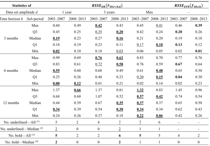
Table 6. Summary statistics of the prediction accuracy of the Ordinary Kriging (OK) model

and the Euro Forward Rates (EFR): pre-crisis (2003–2007) and crisis (2008–2013) sub-periods.

Time horizon h Sub-period 2003–2007 2008–2013 2003–2007 2008–2013 2003–2007 2008–2013 2003–2007 2008–2013

3 months Max 0.60 0.49 0.42 0.43 0.45 0.41 0.46 0.39 Q3 0.45 0.25 0.35 0.20 0.42 0.24 0.20 0.26 Median 0.19 0.23 0.27 0.16 0.21 0.20 0.19 0.18 Q1 0.18 0.19 0.23 0.11 0.17 0.10 0.13 0.12 Min 0.02 0.10 0.18 0.03 0.06 0.05 0.02 0.01 6 months Max 0.99 0.69 0.76 0.62 0.83 0.70 0.77 0.76 Q3 0.83 0.61 0.72 0.58 0.76 0.59 0.67 0.64 Median 0.55 0.60 0.68 0.49 0.61 0.48 0.65 0.50 Q1 0.25 0.26 0.48 0.23 0.20 0.15 0.04 0.30 Min 0.00 0.12 0.01 0.21 0.02 0.14 0.02 0.23 12 months Max 1.37 0.66 1.37 0.81 1.32 0.83 1.45 0.96 Q3 0.68 0.60 1.07 0.52 0.57 0.42 0.74 0.54 Median 0.44 0.39 0.67 0.35 0.37 0.37 0.65 0.50 Q1 0.34 0.39 0.54 0.30 0.34 0.34 0.62 0.43 Min 0.24 0.26 0.37 0.18 0.22 0.06 0.42 0.26 No. underlined—All (1)_{5 2 4 7 7} _{6 - -} No. underlined—Median (2)₂ _{0 0 2 1 1 - -} No. bold—All (3) ₅ _{2 2 6 5 5 4 2} No. bold—Median (4) ₂ _{0 0 2} _{1 1 0 0}

(4)_{Number of median values in bold (total = 3, plus eventual repetitions for d =max).}

This table shows summary statistics of the prediction accuracy of the Ordinary Kriging (OK) model and the Euro Forward Rates (EFR) method used for predicting 30-year maturity Euro Zero Rate, distinguishing between the pre-crisis (2003–2007) and the crisis (2008–2013) sub-periods. Results are presented in terms of root square of each statistic S:{Minimum; 1st Quartile; Median;

3rd Quartile; Maximum} of the models’ squared errors observed at the reference dates (t), defined, respectively, as

̂ _, _, and _{, ,} . RSSEs’ statistics are presented for each combination of sub-periods (2003–2007 and 2008–2013), time horizon h (3, 6 and 12 months) and dataset length d (1, 3 years and max) considered. Underlined statistics have the lowest value among the first three main columns d = 1, d = 3 and d = max (to identify the best d for applying the OK model), while boldface statistics have the lowest value among all the four main columns (to identify the best prediction method between the OK model and the EFR).

Furthermore, we study the performances of the model for different sub-periods from 1 January 2003 and 31 December 2013. Considering the impact of the recent financial crisis on interest rates levels and volatility, we identified a pre-crisis period, ranging from 1 January 2003 to 31 December 2007 (2003–2007), and a full-post crisis period, ranging from 1 January 2008 to 31 December 2013 (2008–2013). We select the 30-year maturity for both EZR and EFR and we assess whether the RSSEs

(18)

are significantly different in the two sub-periods before and during the recent financial turmoil. Table 6 shows the results of our analyses.

The data reported in Table 6 show that, considering both sub-periods, the wider the dataset, the more accurate are the forecasts. We also observe that the OK model (with d = max) outperforms the forward rate method—in terms of lower RSSE statistics—in eight cases out of 15 (about 53%) in the

pre-crisis period, improving further its performances in the crisis period (12 cases out of 15, about

80%). Furthermore, in the crisis period the performances of the OK model are better than its own results in the pre-crisis period, the only exception being for the d = 1 scenario. The higher accuracy of the OK model in the crisis period is probably due to the wider dataset available for the 2008–2013

sub-period, as we observed that its positive effect on the model’s performances increases with d. 5.2. The Extended Dynamic Nelson-Siegel Model

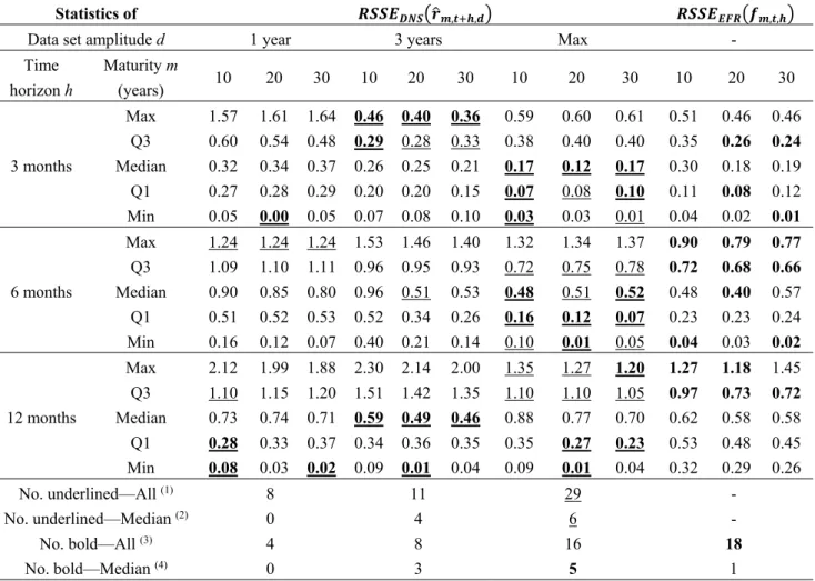
Similarly to the analysis shown in Section 5.1 for the OK model, for each of the 31 combinations [t; d] described in Section 4.2 we apply the DNS method in order to predict the term structure of EZR for all the dates included in the period from 31 December of t to 31 December of the following year (t + 1). Table 7 shows the results of the analysis of accuracy of the DNS model, expressed in terms of

the ̂ _, _, and _{, ,} .

Generally speaking, as the maturity increases, ̂ , , decreases both in the level and in

variability; we also observe that the greater the forecasts’ horizon, the higher are the median errors and the level of uncertainty. In particular, using the max-length dataset, the median ̂ , , is

between 0.18 and 0.30 for predictions of three months ahead, while it rises between 0.40 and 0.62 for six and 12 months ahead-predictions.

Table 7 shows that, also for the DNS model, in most cases the best forecasts are achieved by using the max-length dataset. In particular, when d = max the DNS model outperforms the forward rate method—in terms of lower RSSE statistics (median statistic)—in 19 (5) cases out of 45 (9), against the 33 (7) cases of the OK model.

Our results are in line with the RMSEs determined in previous studies that are based on the DNS model. In particular, it is interesting to compare our RSSE median statistics with the RMSE calculated by Diebold and Li [45] and Chen and Niu [50], as they represent the reference papers for the models considered in our work. To this aim, we focus on the forecasting scenarios with a maturity (m) of 10 years and a time horizon (h) of 6 and 12 months, as they are considered in both in our analyses and in those studies. The results show that our models’ median RSSE are lower than Diebold and Li [45] but higher than Chen and Niu [50], while for h = 3 months (not considered by Diebold and Li [45]) our model performs better also than Chen and Niu [50]. However, the significance of this comparison is limited by the differences existing among each research in terms of errors’ statistics, interest rates (EZR vs. U.S. Treasury yields) and historical periods examined.

Similarly to the analysis shown in Table 6, we study the performances of the DNS model distinguishing between the pre-crisis period (2003–2007) and the full-post crisis period (2008–2013). Hence, we focus on the 30-year maturity for both EZR and EFR and we assess whether the RSSEs are significantly different in the two sub-periods. Table 8 shows the results of our analyses.

(19)

Table 7. Prediction accuracy of the extended dynamic Nelson-Siegel (DNS) model and the

Euro Forward Rates (EFR) forecasting method.

Time horizon h Maturity m (years) 10 20 30 10 20 30 10 20 30 10 20 30 3 months Max 1.57 1.61 1.64 0.46 0.40 0.36 0.59 0.60 0.61 0.51 0.46 0.46 Q3 0.60 0.54 0.48 0.29 0.28 0.33 0.38 0.40 0.40 0.35 0.26 0.24 Median 0.32 0.34 0.37 0.26 0.25 0.21 0.17 0.12 0.17 0.30 0.18 0.19 Q1 0.27 0.28 0.29 0.20 0.20 0.15 0.07 0.08 0.10 0.11 0.08 0.12 Min 0.05 0.00 0.05 0.07 0.08 0.10 0.03 0.03 0.01 0.04 0.02 0.01 6 months Max 1.24 1.24 1.24 1.53 1.46 1.40 1.32 1.34 1.37 0.90 0.79 0.77 Q3 1.09 1.10 1.11 0.96 0.95 0.93 0.72 0.75 0.78 0.72 0.68 0.66 Median 0.90 0.85 0.80 0.96 0.51 0.53 0.48 0.51 0.52 0.48 0.40 0.57 Q1 0.51 0.52 0.53 0.52 0.34 0.26 0.16 0.12 0.07 0.23 0.23 0.24 Min 0.16 0.12 0.07 0.40 0.21 0.14 0.10 0.01 0.05 0.04 0.03 0.02 12 months Max 2.12 1.99 1.88 2.30 2.14 2.00 1.35 1.27 1.20 1.27 1.18 1.45 Q3 1.10 1.15 1.20 1.51 1.42 1.35 1.10 1.10 1.05 0.97 0.73 0.72 Median 0.73 0.74 0.71 0.59 0.49 0.46 0.88 0.77 0.70 0.62 0.58 0.58 Q1 0.28 0.33 0.37 0.34 0.36 0.35 0.35 0.27 0.23 0.53 0.48 0.45 Min 0.08 0.03 0.02 0.09 0.01 0.04 0.09 0.01 0.04 0.32 0.29 0.26 No. underlined—All (1)₈ ₁₁ ₂₉ _- No. underlined—Median (2)₀ ₄ ₆ _- No. bold—All (3)₄ ₈ ₁₆ ₁₈ No. bold—Median (4)₀ ₃ ₅ ₁

(1)_{Number of underlined statistics (total = 45, plus eventual repetitions for d=max);}

(2)_{Number of underlined median values (total = 9, plus eventual repetitions for d=max);}

(3)_{Number of statistics in bold (total = 45, plus eventual repetitions for d=max);}

(4)_{Number of median values in bold (total = 9, plus eventual repetitions for d=max).}

This table shows summary statistics of the prediction accuracy of the extended dynamic Nelson-Siegel (DNS) model and the Euro Forward Rates (EFR) forecasting method. Results are presented in terms of root square of each statistic S:{Minimum; 1st Quartile; Median; 3rd Quartile; Maximum} of the models’ squared errors

observed at the reference dates (t), defined, respectively, as ̂ , , and , , . RSSEs’

statistics are presented for each combination of maturity (m = 10, 20 and 30 years), time horizon h (3, 6 and 12 months) and dataset length d (1, 3 years and max) considered. Underlined statistics have the lowest value among the first three columns d = 1, d = 3 and d = max (to identify the best d for applying the DNS model), while boldface statistics have the lowest value among all the four columns (to identify the best prediction method between the DNS model and the EFR).

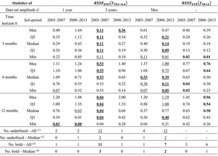
The results shown in Table 8 confirm that, considering both sub-periods, also for the DNS model the wider the dataset, the more accurate are the forecasts. However, a relevant difference emerges between the two sub-periods, as in the pre-crisis and the full-post crisis periods the best scenarios are, respectively, d =3 and d = max. However, since for d = 3 only one forecast could be developed (due to the availability of the data required for applying the DNS model), for the pre-crisis scenario reference shall be made to the more significant d = max scenario. We observe that the DNS model (with

(20)

d = max) outperforms the forward rate method—in terms of lower RSSE statistics—in five cases out of

15 (about 33%) in the pre-crisis period and in eight cases out of 15 (about 53%) in the crisis period.

Table 8. Summary statistics of the prediction accuracy of the extended dynamic

Nelson-Siegel (DNS) model and the Euro Forward Rates (EFR): pre-crisis (2003–2007) and crisis (2008–2013) sub-periods.

Time horizon h Sub-period 2003–2007 2008–2013 2003–2007 2008–2013 2003–2007 2008–2013 2003–2007 2008–2013 3 months Max 0.40 1.64 0.11 0.36 0.61 0.47 0.46 0.39 Q3 0.35 1.12 0.11 0.34 0.52 0.21 0.20 0.26 Median 0.29 0.43 0.11 0.27 0.40 0.14 0.19 0.18 Q1 0.26 0.36 0.11 0.19 0.30 0.09 0.13 0.12 Min 0.22 0.05 0.11 0.10 0.11 0.01 0.02 0.01 6 months Max 1.11 1.24 0.53 1.40 1.37 1.00 0.77 0.76 Q3 1.10 1.06 0.53 0.96 1.04 0.72 0.67 0.64 Median 1.09 0.71 0.53 0.65 0.53 0.39 0.65 0.50 Q1 0.78 0.55 0.53 0.22 0.38 0.11 0.04 0.30 Min 0.07 0.52 0.53 0.14 0.07 0.05 0.02 0.23 12 months Max 1.20 1.88 0.04 2.00 1.20 1.19 1.45 0.96 Q3 1.00 1.35 0.04 1.53 0.88 1.00 0.74 0.54 Median 0.76 0.62 0.04 0.68 0.37 0.77 0.65 0.50 Q1 0.54 0.41 0.04 0.42 0.26 0.40 0.62 0.43 Min 0.02 0.08 0.04 0.28 0.04 0.21 0.42 0.26 No. underlined—All (1)₂ _{2 12 1 4 12 - -} No. underlined—Median (2)₀ ₁ ₃ _{0 1 2 - -} No. bold—All (3)_{1 1 11} _{1 1 7} _{3 6} No. bold—Median (4)_{0 0 3} _{0 1 2} _{0 1}

(4)_{Number of median values in bold (total = 3, plus eventual repetitions for d = max).}

This table shows summary statistics of the prediction accuracy of the extended dynamic Nelson-Siegel (DNS) model and the Euro Forward Rates (EFR) method used for predicting 30-year maturity Euro Zero Rate, distinguishing between the pre-crisis (2003–2007) and the crisis (2008–2013) sub-periods. Results are presented in terms of root square of each statistic S:{Minimum;

1st Quartile; Median; 3rd Quartile; Maximum} of the models’ squared errors observed at the reference dates (t), defined,

respectively, as ̂ , , and , , . RSSEs’ statistics are presented for each combination of sub-periods (2003–2007 and 2008–2013), time horizon h (3, 6 and 12 months) and dataset length d (1, 3 years and max) considered. Underlined statistics have the lowest value among the first three main columns d = 1, d = 3 and d = max (to identify the best d for applying the DNS model), while boldface statistics have the lowest value among all the four main columns (to identify the best prediction method between the DNS model and the EFR).

(21)

5.3. The Comparison between the OK Model and the DNS Model

Both the OK and the DNS models were applied to predict the EZR considering the same subset of historical observations at each forecasting date. Therefore, the statistics of RSSE shown in Tables 5 and 7, respectively, can be directly compared in order to identify the model that is characterized by the highest level of accuracy, i.e., the lowest RSSE. Table 9 shows the results of the comparative analysis between the OK model and the DNS model.

Table 9. Comparative analysis of prediction accuracy between the Ordinary Kriging (OK)

model and the extended dynamic Nelson-Siegel (DNS) model.

Model Model with the Lowest Statistic of , ,

Data set amplitude d 1 year 3 years Max

Time horizon h Maturity m (years) 10 20 30 10 20 30 10 20 30 3 months Max OK OK OK OK DNS DNS OK OK OK Q3 OK OK OK DNS OK OK OK OK OK Median OK OK OK DNS OK OK DNS DNS DNS Q1 OK OK OK OK OK DNS DNS OK DNS Min DNS DNS OK OK OK OK OK DNS DNS 6 months Max OK OK OK OK OK OK OK OK OK Q3 OK OK OK OK OK OK OK OK OK Median OK OK OK OK OK DNS OK OK DNS Q1 OK OK OK OK OK OK DNS DNS DNS Min OK OK OK OK OK OK DNS DNS OK 12 months Max OK OK OK OK OK OK OK OK DNS Q3 OK OK OK OK OK OK OK OK OK Median OK OK OK OK DNS OK OK OK OK Q1 OK OK OK OK DNS OK OK OK DNS Min DNS DNS DNS DNS DNS DNS OK DNS DNS No. OK—All 40 34 28 No. DNS—All 5 11 17 No. OK—Median 9 6 5 No. DNS—Median 0 3 4

This table shows the results of a comparative analysis of prediction accuracy between the Ordinary Kriging (OK) model and the extended dynamic Nelson-Siegel (DNS) model. The level of prediction accuracy is measured in terms of root square of each statistic S:{Minimum; 1st Quartile; Median; 3rd Quartile; Maximum}

of the models’ squared errors observed at the reference dates (t), defined, respectively, as ̂ , ,

and ̂ , , . For each combination of maturity (m = 10, 20 and 30 years), time horizon h (3, 6

and 12 months) and dataset length d (1, 3 years and max) considered the table indicates the model characterized by the lowest statistic of RSSE, therefore the model characterized by the highest level of prediction accuracy.

Focusing on the distinction between the pre-crisis and the full-post crisis periods, Table 10 shows the results of the comparative analysis between the OK model and the DNS model based on the statistics of RSSE reported in Tables 6 and 8.

(22)

Table 10. Comparative analysis of prediction accuracy between the Ordinary Kriging (OK)

model and the extended dynamic Nelson-Siegel (DNS) model: pre-crisis (2003–2007) and crisis (2008–2013) sub-periods.

Time horizon h Sub-period 2003–2007 2008–2013 2003–2007 2008–2013 2003–2007 2008–2013 2003–2007 2008–2013 3 months Max DNS OK DNS DNS OK OK DNS OK Q3 DNS OK DNS OK OK DNS DNS OK Median OK OK DNS OK OK DNS OK OK Q1 OK OK DNS OK OK DNS OK OK Min OK DNS DNS OK OK DNS OK DNS 6 months Max OK OK DNS OK OK OK OK OK Q3 OK OK DNS OK OK OK OK OK Median OK OK DNS OK DNS DNS OK OK Q1 OK OK OK DNS OK DNS OK OK Min OK OK OK DNS OK DNS OK OK 12 months Max DNS OK DNS OK DNS OK DNS OK Q3 OK OK DNS OK OK OK OK OK Median OK OK DNS OK DNS OK OK OK Q1 OK OK DNS OK DNS OK OK OK Min DNS DNS DNS OK DNS OK DNS DNS No. OK—All 11 13 2 12 10 8 11 13 No. DNS—All 4 2 13 3 5 7 4 2 No. OK—Median 3 3 0 3 1 1 3 3 No. DNS—Median 0 0 3 0 2 2 0 0

This table shows the results of a comparative analysis of prediction accuracy between the Ordinary Kriging (OK) model and the extended dynamic Nelson-Siegel (DNS) model. The analysis is focused on the 30-year maturity Euro Zero Rate, distinguishing between the pre-crisis (2003–2007) and the crisis (2008–2013) sub-periods. The level of prediction accuracy is measured in terms of root square of each statistic S:{Minimum; 1st Quartile; Median; 3rd Quartile; Maximum} of the models’ squared errors observed at the reference dates (t), defined, respectively, as ̂ _, _, and ̂ _, _, . For each combination of

sub-periods (2003–2007 and 2008–2013), time horizon h (3, 6 and 12 months) and dataset length d (1, 3 years and max)

considered, the table indicates the model characterized by the lowest statistic of RSSE, therefore the model characterized by the highest level of prediction accuracy.

To facilitate the visual comparison of the efficacy of each forecasting method, Figure 4 represents the statistics shown in Tables 5 and 7 using box plot graphics. For sake of brevity, the corresponding graphic is not reported for Tables 6 and 8.

We observe that for all the scenarios of dataset length—1 year, 3 years and max—the RSSE statistics (median statistic) of ̂ _, _, are lower for the OK model in the majority of cases, that is in 40 (9), 34 (6) and 28 (5) cases out of 45 (9), respectively. Focusing on the d = max scenario, as it revealed to be the optimal dataset length for both the models, for 12 months ahead forecasts the OK model was more accurate than the DNS model in 11 (3) cases out of 15 (3).

(23)

Figure 4. Box plots of the statistics shown in Tables 5 and 7 of the values of

̂ , , , ̂ , , and , , at each time t for each

maturity (m = 10, 20 and 30 years), for each time horizon h (3, 6 and 12 months) and by dataset length d (1, 3 years and max).

Relating to the sub-periods analysis, the OK model outperforms the DNS model—in terms of lower RSSE statistics—in 23 cases out of 45 (about 51%) in the pre-crisis period and in 33 cases out of 45 (about 73%) in the crisis period. Therefore, in terms of prediction accuracy, the OK model is in line

(24)

with the DNS model in the pre-crisis period, while a slight improvement can be observed for the crisis period from 2008 to 2013.

6. Conclusions

This paper contributes to the existing literature by adopting an innovative approach to analyze the term structure of interest rates for short-term forecasting purposes. Our work is the first to develop a spatial statistical analysis of interest rates time series, outlining a procedure to calculate the empirical anisotropic variogram of Euro Zero Rates, to fit and select a theoretical variogram model and to use it to forecast the term structure up to 12 months using Ordinary Kriging.

The empirical results referring to Euro Zero Rates in the period 2003–2014 show that, for long-term maturities, the proposed model is characterized by good levels of forecasting accuracy, with prediction errors that increase as a greater time horizon is considered. From a comparative point of view, our model proves to be more accurate than using the forward rates implicit in the Euro Zero Rates curve as proxies of the market expectations of future interest rates and the best results are achieved when all the historical observations are used to build up the model. Furthermore, the comparison with the dynamic Nelson-Siegel model (based on Chen and Niu [50] and Diebold and Li [45]) shows that in some cases the proposed model is slightly more precise, with special reference to the 12 months-ahead forecasts.

In future studies, our approach could be refined in various directions. First of all, future studies could extend the comparative analysis of efficacy to other interest rate forecasting models. Secondly, it would be interesting to test the performances of the proposed model in longer-term predictions going beyond the 12 months horizon to which we limited the present study. Finally, the proposed method could be applied and tested also for other yield curves and historical periods.

Author Contributions

The authors contributed equally to this work.

Conflicts of Interest

The authors declare no conflict of interest.

References

1. Hunt, P.; Kennedy, J.; Pelsser, A. Markov-Functional Interest Rate Models. Financ. Stoch. 2000,

4, 391–408.

2. Hamilton, J.D. Time Series Analysis; Princeton University Press: Princeton, NJ, USA, 1994. 3. Cressie, N. Statistics for Spatial Data; Wiley: New York, NY, USA, 1993.

4. Shabenberger, O.; Gotway, C. Statistical Methods for Spatial Data Analysis; Chapman & Hall/CRC: Boca Raton, FL, USA, 2005.

5. Fernández-Avilés, G.; Montero, J.M.; Orlov, A.G. Spatial modeling of stock market comovements.

Financ. Res. Lett. 2012, 9, 202–212.

6. Remolona, E.M.; Wooldridge, P.D. The euro interest rate swap market. BIS Q. Rev. 2003, March, 47–56.

(25)

7. Brigo, D.; Mercurio, F. Interest Rate Models-Theory and Practice: With Smile, Inflation and

Credit; Springer Finance: Berlin, Germany, 2007.

8. Subrahmanyam, M.G. The Term Structure of Interest Rates: Alternative Approaches and their Implications for the Valuation of Contingent Claims. Geneva Pap. Risk. Insur. Theory 1996, 21, 7–28. 9. Black, F.; Scholes, M. The Pricing of Options and Corporate Liabilities. J. Political Econ. 1973,

81, 637–654.

10. Merton, R.C. An Intertemporal Capital Asset Pricing Model. Econometrica 1973, 41, 867–887. 11. Brennan, M.J.; Schwartz, E.S. A Continuous Time Approach to the Pricing of Bonds. J. Bank.

Financ. 1979, 3, 133–155.

12. Ho, T.S.; Lee, S.B. Term Structure Movements and Pricing Interest Rate Contingent Claims.

J. Financ. 1986, 41, 1011–1029.

13. Hull, J.; White, A. Pricing Interest-Rate-Derivative Securities. Rev. Financ. Stud. 1990, 3, 573–592.

14. Heath, D.; Jarrow, R.; Morton, A. Bond Pricing and the Term Structure of Interest Rates: A New Methodology for Contingent Claims Valuation. Econometrica 1992, 60, 77–105.

15. Brace, A.; Gatarek, D.; Musiela, M. The Market Model of Interest Rate Dynamics. Math. Financ.

1997, 7, 127–155.

16. Brace, A.; Musiela, M. A Multifactor Gauss Markov Implementation of Heath, Jarrow, and Morton. Math. Financ. 1994, 4, 259–283.

17. Goldys, B.; Musiela, M.; Sondermann, D. Lognormality of Rates and Term Structure Models.

Stoch. Anal. Appl. 2000, 18, 375–396.

18. Musiela, M. General Framework for Pricing Derivative Securities. Stoch. Proc. Appl. 1995, 55, 227–251.

19. Musiela, M.; Rutkowski, M. Continuous-Time Term Structure Models: Forward Measure Approach.

Financ. Stoch. 1997, 1, 261–291.

20. Duffie, D.; Singleton, K.J. Modeling Term Structures of Defaultable Bonds. Rev. Financ. Stud.

1999, 12, 687–720.

21. Jamshidian, F. LIBOR and Swap Market Models and Measures. Financ. Stoch. 1997, 1, 293–330. 22. De Jong, F.; Driessen, J.; Pelsser, A. Libor Market Models versus Swap Market Models for

Pricing Interest Rate Derivatives: An Empirical Analysis. Eur. Financ. Rev. 2001, 5, 201–237. 23. Longstaff, F.A.; Schwartz, E.S. Interest Rate Volatility and the Term Structure: A Two-Factor

General Equilibrium Model. J. Financ. 1992, 47, 1259–1282.

24. Cox, J.C.; Ingersoll, J.E.; Ross, S.A. A Re-Examination of Traditional Hypotheses about the Term Structure of Interest Rates. J. Financ. 1981, 36, 769–799.

25. Cox, J.C.; Ingersoll, J.E.; Ross, S.A. An Intertemporal General Equilibrium Model of Asset Prices.

Econometrica 1985, 53, 363–384.

26. Cox, J.C.; Ingersoll, J.E.; Ross, S.A. A Theory of the Term Structure of Interest Rates.

Econometrica 1985, 53, 385–407.

27. Vasicek, O. An Equilibrium Characterization of the Term Structure. J. Financ. Econ. 1977, 5, 177–188.

28. Black, F.; Karasinski, P. Bond and Option Pricing when Short Rates are Lognormal. Financ. Anal. J.