NNFISS - LP3 - 033 L 1 39
Titolo
Validazione del modulo di cinetica KIN3D di ERANOS. Analisi per i sistemi GODIVA e GUINEVERE.
Descritlori
Tipologia del documento: Rapporto Tecnico
Collocazione contrattuale: Accordo di programma ENEA-MSE: tema di ricerca "Nuovo nucleare da fissione"
Argomenti trattati: Cod ice ERANOS - Modulo KIN3D Cinetica neutronica di nocciolo Metodi Deterministici
Sommario
II modulo KIN3D del sistema di calcolo francese ERANOS
e
stato sviluppato alia fine degli anni 90 per I'analisi di cinetica neutronica di sistemi critici e sottocritici. Per quanto riguarda Ie campagne sperimentali europee in supporto della tecnologia ADS I'attenzionee
attualmente focalizzata sui programma sperimentale GUINEVERE, lanciato ne12007. II progetto GUINEVERE confluira nel progetto FREYA, partito a marzo 2011, del 7 Programma Quadro della CEoII presente lavoroe
incentrato SUlia validazione del modulo ERANOS/KIN3D sia per un sistema classico quale GODIVA sia per una configurazione di nocciolo rappresentativa del programma GUINEVERE/FREYA.Summary
The KI N3D module of the ERANOS French code was developed at the end of the 1990s to analyse the neutron kinetic behaviour of both critical and subcritical systems. Concerning European experiments in support of ADS technology, presently the attention is focused on the GUINEVERE experimental program,
launched in 2007. The GUINEVERE project will flow into the FREYA project, started on March 2011, of the Seventh EU Framework Programme. This report is focused on the test of the ERANOS/KIN3D system to both a classic benchmark like GODIVA and to one core configuration representative of the
GUINEVERE/FREYA program.
Note
Autori: G. Bianchini, N.Burgio, M. Carta, V. Fabrizio, V. Peluso, L. Ricci
Questo lavoro
e
stato effettuato nell'ambito dell'Accordo ENEA-MSE - Area: Governo, Gestione e Sviluppo del Sistema Elettrico Nazionale - Tematica di Ricerca: Energia Nucleare - Progetto 1.3 NUOVO NUCLEARE DA FISSIONE: COLLABORAZIONIINTERNAZIONALI E SVILUPPO COMPETENZE IN MATERIANUCLEARE - LINEA PROGETTUALE 3: Reattori di IV generazione - Obiettivo E2 (PAR 2008-9).
Copia n. In carico a:
2 NOME
FIRMA
1 NOME
FIRMA
0
~/iVM
NOME M.CARTA P. MELONI P.MELONIEMISSIONE
Pf ~
~
~~ ~FIRMA
INDEX 1. Introduction ... 3 2. ERANOS/KIN3D module ... 3 2.1 Generalities ... 3 2.2 Code architecture ... 3 2.3 Cell calculations ... 4 2.4 Static calculations ... 5
2.5 Kinetics calculations: KIN3D module ... 5
3. Reactivity measurement methods ... 6
3.1 Preface ... 6
3.2 Slope (or α-fitting) method ... 7
3.3 Area-ratio methods ... 7
3.4 Source-jerk and Beam-jump methods ... 8
3.4.1 Beam-jump method ... 8
3.4.2 Source-jerk method ... 9
3.5 Analogies between Area-ratio and Source-jerk/Beam-jump methods ... 9
4. GODIVA analysis... 12
4.1 GODIVA configurations ... 12
4.2 Kinetics calculation specifications ... 14
4.3 Results ... 16 4.3.1 GODIVA Bare ... 16 4.3.2 GODIVA+Copper ... 18 4.3.3 GODIVA+Lead ... 20 5. GUINEVERE analysis ... 22 5.1 Generalities ... 22
5.2 ERANOS calculation model set-up ... 26
5.2.1 Cross section sets generation by the ECCO module ... 26
5.2.2 Reactor modelling ... 29
5.3 Kinetics calculation specifications ... 31
5.4 Results ... 33
5.5 ERANOS/KIN3D-MCNPX results comparison. ... 35
6. Conclusions ... 37
7. References ... 38
1. Introduction
The KIN3D module [1] of the ERANOS French code [2] was developed at the end of the 1990s to analyse the neutron kinetic behaviour of both critical and subcritical systems. Recently an increasing interest towards neutron kinetic analysis by the ERANOS/KIN3D system has been in Accelerator Driven Systems (ADS) field, with regard to the interpretation of pulsed source techniques for the measurement of the subcritical level in the frame of zero-power MUSE [3] and YALINA [4] experimental campaigns.
Concerning experiments in support of ADS technology, presently the attention is focused on the GUINEVERE experimental program [5], launched in 2007 as European project included in the
Integrated Project (IP) EUROTRANS1 of the Sixth EU Framework Programme. The GUINEVERE
project will flow into the FREYA project [6], started on March 2011, of the Seventh EU Framework Programme.
This report is focused on the test of the ERANOS/KIN3D system to both a classic benchmark like GODIVA [7] and to one core configuration representative of the GUINEVERE/FREYA program.
2. ERANOS/KIN3D module
2.1 Generalities
The European Reactor Analysis Optimized calculation System, ERANOS, has been developed and validated with the aim of providing an appropriate basis for neutronic calculations of fast (and thermal) reactor cores. It consists of data libraries, deterministic codes and calculation procedures developed within a European framework and it meets the needs expressed by the industrialists and the teams working on the design of fast reactors, present and future.
ERANOS is written using the ALOS software which requires only standard FORTRAN compilers and include advanced programming features. It allows, with the use of LU user’s language, to perform programs of R&D in reactor physics without needing specific development.
2.2 Code architecture
Fast reactor core, shielding and fuel cycle calculations can be performed by the ERANOS system. A modular structure was adopted for easier evolution and incorporation of new functionalities. Blocks of data can be created (data SETs) or used by different modules or by the user with LU control language. Programming and dynamic memory allocation are performed with the use of the ESOPE language. It can be possible to make an external temporary storage or permanent storage with the GEMAT and ARCHIVE functions, respectively. ESOPE, LU, GEMAT, and ARCHIVE are all part of the ALOS software.
This type of structure, based on modular system, allows to link together different modules in procedures corresponding to recommended calculation routes ranging from fast-running and moderately-accurate ‘routine’ procedures to slow-running but highly-accurate ‘reference’ procedure.
The main contents of ERANOS-2.0/2.1 package are:
nuclear data libraries, multigroup cross-sections from the ERALIB1, ENDF-/B-VI.8, JEF-2.2, JEF-3.1 evaluated nuclear data file, and other specific data;
a cell and lattice code ECCO [8];
reactor flux solvers (diffusion, Sn transport, nodal variational transport);
a burn-up module;
different processing modules (material and neutron balance, breeding gains,…); perturbation theory and sensitivity analysis modules;
core follow-up modules;
a fine burn-up analysis subset named MECCYCO (mass balances, activities, decay heat, dose rate).
Each nuclear data library contains four neutron cross section libraries obtained by processing corresponding nuclear data files with the NJOY and CALENDF codes and they are:
a 1968-group library that contains 41 main nuclides;
a 33-group library that contains 246 nuclides, including pseudo fission products; a 175-group library used for shielding calculation only;
a 172-group library used mainly for thermal spectrum calculations. 2.3 Cell calculations
ERANOS consists of data libraries, deterministic codes and calculation procedures which have been developed within the European Collaboration on Fast Reactors over the past 30 years or so.
ERANOS is a deterministic code system, so neutron physics calculations are performed at the cell/lattice level and at the core level. The development of the ECCO Code was decided in 1985 by several R&D teams working within the framework of the European Fast Reactor Collaboration (see for example [9]).
ECCO, European Cell COde, is the cell code that allows to calculate the cross sections and matrices for use them in a core calculation performed by the other ERANOS modules.
First of all, it is necessary to create media (homogeneous regions), physical description, concentrations of the different isotopes, expansion coefficients and the geometric description of the cell. Then the cross sections are calculated by using the defined media and the nuclear libraries by means of the collision probability method. An ECCO calculation corresponds to a succession of STEPs and for each STEP one can choose energy structure, geometry (heterogeneous or homogeneous), processing of the flux or balance, self-shielding, and so on.
Several types of geometry are available within the ECCO code:
1D, plane or cylindrical with exact collision probabilities method;
2D, rectangular lattice of cylindrical and/or square pins within a square tube, hexagonal lattice of cylindrical pins within an hexagonal wrapper with approximate collision probability by Roth and double step method;
3D, slab with the sides of the boxes and the tube described explicitly with approximate collision probability method.
The user has the possibility to chain several calculation steps so as to produce design or reference calculations, or even to use specific capabilities, according to the need of the study.
A route is a recommended way to perform the ECCO calculation. The first route is the “reference” route that does not care about the computing time and treats the heterogeneous cell at energy fine group level (1968 groups). The second route is the “project” or “design” route in which some simplifying hypotheses are made, the elastic slowing down is treated in a homogeneous geometry but at the fine group level, the self-shielding is treated in a heterogeneous geometry at the broad group level (33 groups).
2.4 Static calculations
For all the geometries, 1D plane, cylindrical and spherical, 2D RZ, R-θ, rectangular lattice XY, hexagonal lattice, and 3D rectangular lattice XYZ, hexagonal-Z can be used finite difference diffusion solvers.
In 1D geometries and in some 2D geometries like RZ and XY can be performed finite difference Sn
transport calculations by the BISTRO [10] code.
The physics of thermal and fast reactors requires the capability to solve the transport equation in accurate manner for different 2D and 3D geometries; nodal methods are well adapted for these topics because of the reduced numbers of unknowns used and the good accuracy in the solution by using high order approximation for spatial and angular expansions of the flux and current in node. Both 2D (XY and hexagonal) and 3D (XYZ and hexagonal-Z) geometries are available with TGV/VARIANT [11] module; this method is based on the second order from of the even-parity transport equation. VARIANT module was developed for solving the steady-state multigroup neutron diffusion and transport equations for core calculation in both geometries 2D and 3D, it performs direct flux calculation, with or without an external source, and adjoint calculation and is possible to set up several parameters for different types of calculations. The code incorporates a number of attractive features, such as a clear hierarchy of space-angle approximations, well-behaved small mesh limits and the absence of both ray effects and the artificial diagonal streaming depression. The computing time in comparison with other methods for solving the transport equation (Sn, Monte-Carlo) is more efficient along with the reliability and accuracy reached in
finding the solution.
2.5 Kinetics calculations: KIN3D module
In reactor analysis an important role is played by the simulation of reactor transients. This is important not only to predict the reactor behaviour under operational conditions but mostly to evaluate consequences of hypothetical accidents. The interpretation of reactor experiments requires the study of reactor kinetics, and these are addressed in ERANOS by KIN3D [1] module.
The treatment of the time dependence in neutron kinetics is generally based on two models: point and space-time kinetics.
In the point kinetics model the flux shape, that determines power shape and reactivity coefficients, is assumed to be constant during the transient; in the space-time kinetic calculations we have three different models: direct, adiabatic and quasi-static schemes.
In the conventional point-kinetics method, the flux is written as the product of an amplitude function and a shape function:
) 0 , , , ( ) ( ) , , , (r E t P t r E t
The kinetics parameters are calculated for the initial steady-state conditions, then during the transient the code calculates the reactivity and solves the point kinetics equations with two different time grid, one coarse for reactivity calculations associated with a reactivity step and one fine grid for solving point-kinetics equations associated with an amplitude step.
When an external source problem is solved, the external source shape is not changed during the transient. The source characteristics, which are initially evaluated for the steady-state conditions, are updated only in amplitude.
The direct method uses a straightforward time discretization of the time-dependent neutron transport or diffusion equation. The adiabatic and quasi-static space time schemes are based on the fact that the flux shape does not have to be update as frequently as the flux amplitude, so it can be used the following equation:
) , , , ( ) ( ) , , , (r E t P t r E tn
where the flux amplitude P(t) is calculated with small time steps and the flux shape ψ is calculated less frequently, and tn is the time point when the flux shape has been last recalculated. The flux
shape update provides a new power distribution and reactivity coefficients.
The adiabatic method may result in an erroneous flux shape evaluation when reactor parameters change frequently because the flux shape is approximate at time tn solving the homogeneous or
inhomogeneous steady-state transport or diffusion equations.
In the quasi-static scheme the flux shape is obtained from an “associated” flux, estimated by the direct method using a time step equal to the shape step (Fig. 1).
Figure 1 – Time grids used in the adiabatic and improved quasi-static schemes [1].
The flux amplitude, which is obtained by solving the point-kinetics equations, is used as a fitting function for the flux shape calculations in the improved quasi-static scheme.
In this work point kinetics and direct (reference) methods shall be taken into account for the analyses.
3. Reactivity measurement methods
3.1 Preface
As previously mentioned an increasing interest towards neutron kinetic analysis by the ERANOS/KIN3D system has been in Accelerator Driven Systems (ADS) field, with regard to the interpretation of Pulsed Neutron Source (PNS) techniques for the measurement of the subcritical level in zero-power cores. In this chapter a short review of three experimental techniques for the determination of the reactivity level in subcritical systems will be provided, being such a kind of
system neutron response to some external source transient the test-bench for the KIN3D module behaviour.
3.2 Slope (or α-fitting) method
When a short pulse of neutrons is injected into a subcritical reactor, and the neutron flux is measured by means of a neutron detector, a typical output of the detector response is composed by a fast peak that dies out very rapidly, followed by a slower decay. The faster response represents the contribution of the prompt modes to the detector reading whereas the second slower response represents the effect of delayed-neutron emission. In the prompt neutrons time zone, after dying out of the higher harmonics, a pure exponential behaviour (after subtracting steady delayed neutron background) of the type P(t)=P0∙exp(αpt) takes place, with time constant αp given by:
eff p (1)
The triad reactivity ρ, effective delayed neutron fraction βeff, mean neutron generation time Λ
characterizes the slope of the prompt neutrons response. Measuring the slope αp, and knowing -or
having estimates of- βeff and Λ independently by other measurements, it's possible to obtain the
system reactivity ρ by Eq. (1).
PNS α-fitting method requires an accurate evaluation of the "expected" αp, and of the associated
neutron mean generation time Λ, to take into account kinetics distortion effects resulting in different flux shapes respect to those predicted by eigenvalue calculations.
For what concerns the PNS α-fitting method it is possible, when looking at experimental data, to foresee "a priori" three classes of possible responses to a short pulse:
a) The system responses exhibit the same predominant one-exponential slope for all the positions (core, reflector, and shield). The system seems to act as a point, and point kinetics seems to be applicable without correction factors.
b) For a given position (core, reflector, shield), the system response exhibits a predominant one-exponential slope, but such slopes are different if compared one each other. Thus, at least a "local" point kinetics behaviour is observed: α-fitting methods, which invoke for an estimate of the neutron mean generation time Λ, will provide reactivity values (in dollars) apparently depending on the detector position. Correction factors are required.
c) The system responses do not exhibit predominant one-exponential slopes: only fitting procedures on the experimental data can try to smooth the problem, in the effort to reproduce, if possible, situations similar to case b). Correction factors are required.
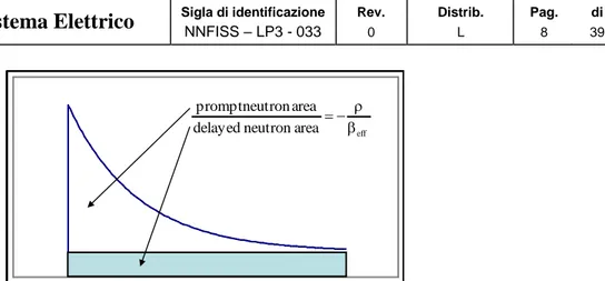
3.3 Area-ratio methods
Analogously to α-fitting method, PNS Area-ratio methods are based on the analysis of the responses shown by a subcritical system to an external source pulse. A typical response of this kind is shown in Fig. 2, where the contributions of prompt and delayed neutrons are evidenced.
eff area neutron delayed area neutron prompt eff area neutron delayed area neutron prompt
Figure 2 –Response shown by a subcritical system to an external neutron source pulse.
In particular, the fundamentals of the Area-ratio method [12] consist in the evaluation of the absolute level of reactivity (in dollars) by measuring, independently by the detector position, the ratio between the area under the prompt peak and the delayed one after the injection of a neutron pulse in the subcritical system:
d d t $ I I -I area neutron Delayed area neutron Prompt ρ (2)
where the prompt area Ip = It-Id is equal to the difference between the total area It and the delayed
one. If the system response cannot be approximated by point kinetics, the reactivity value can
apparently depend on the detector position rD2, and we’ll obtain, in place of Eq. (2), relationships
like:
D d D d D t D $ I I -I area neutron delayed Local area neutron prompt Local ρ r r r r In such cases these spatial effects can be taken into account by calculating spatial correction factors obtained by:
1. Equivalent steady state methods obtained by solving time-independent inhomogeneous transport problems [13] (see for example [3] for an application to the MUSE-4 case).
2. Explicit time dependent analysis where time-dependent inhomogeneous transport problems are solved by KIN3D module (this work).
3.4 Source-jerk and Beam-jump methods
3.4.1 Beam-jump method
Let us consider the classical point kinetics equations (written in classical notation):
) ( ) ( ) ( ) ( ) ( ) ( ) ( , , , , t P t C dt t dC t S t C t P dt t dP eff i eff i i eff i eff eff i i i eff
2 rFor the steady state corresponding to the source Sh we have: h eff i h eff i i h eff h P C S P , , (3)
After a sudden variation of the source from Sh to S1 we have:
eff p t eff eff eff h t h p p e S P e P t P 1 ) ( 1Assuming constant the delayed background, after some |1/αp| seconds the flux amplitude P(t)
reaches a meta-stable state given by:
eff eff eff h S P P 1 1
By comparison with Eq. (3) we have:
h eff h eff eff eff h h S S S P P P1 1 (4)
Eq. (4) links the flux amplitude variation to the external source variation through the system reactivity (in dollar units).
3.4.2 Source-jerk method
This particular case is obtained setting S1eff=0 in Eq. (4) and obtaining:
eff h h P P P 1 or: eff eff h P P1
3.5 Analogies between Area-ratio and Source-jerk/Beam-jump methods
All the dynamic methods described in the preceding sections are based on the validity of the so-called point reactor approximation. As well known, for the point-reactor model of a time-dependent problem, the flux Ф(r, Ω, E, t) is written as the product of an amplitude factor P(t), which is dependent on time only, and a shape factor (or shape function) ψ(r, Ω, E) independent of time. Under these assumptions, it is possible to write the reactor kinetics equations as:
) ( ) ( ) ( ) ( ) ( ) ( ) ( , , , , t P t C dt t dC t S t C t P dt t dP eff i eff i i eff i eff eff i i i eff
with:
dE ) E, , ( E) , ( ) E, , ( dE' dE ) , E' , ( ) E' , ( (E) ) E, E' , ( ) E, , ( 1 0 0 Ω r Ω r r Ω r Ω' Ω r Ω' r r Ω Ω' r Ω r d d d d d F x f x f
and: dE t) , E, , ( ) E, , ( 1 ) ( dE t) , ( (E) ) E, , ( 1 ) ( dE' dE ) , E' , ( ) E' , ( (E) ) E, , ( 1 dE ) E, , ( 1 ) E, , ( 1 0 0 , , 0 , 0 Ω r Ω r Ω r Ω r r Ω r Ω' Ω r Ω' r r Ω r Ω r Ω r Ω r d d S F t S d d C F t C d d d F d d v F eff i i eff i eff i i eff f i i eff i
The adjoint flux Ф0+ is relative to a critical reference state and the Δ’s represent the differences
between the respective quantities, Σ and Σf, in the perturbed state and in the critical reference state.
The factor F is more or less arbitrary, and it has no effect on the solutions to the reactor kinetics equations since it always cancels in the numerator and denominator of each term. In practice, however, F is chosen so that the various parameters have a physical interpretation for simple situations. A reasonable choice for F is:
dE' d dE d d ) , E' , ( ) E' , ( (E) ) E, , ( F
0 r Ω f r r Ω' r Ω Ω'If we assume that the shape function ψ has the same dependence on r, Ω and E as the fundamental angular flux eigenfunction Ф0(r, Ω, E) for the reference critical system, or alternatively we rely on
the orthogonalization properties of the selected adjoint flux over the shape function in order to extract from the flux shape the fundamental component, we obtain for the ρ parameter the classical relation: k 1 -k
In principle we are not constrained to have a critical reference state. In fact, if we assume as reference state a generic subcritical state characterized by the eigenvalue k, with the associated adjoint flux Ф+
(r, Ω, E), under analogous assumptions we can write similar equations to those shown above where now the reactivity is given by:
k' k k'-k and k’ is the eigenvalue of the perturbed state.
In general, the shape function is not independent on time, i.e. the neutron flux separability hypothesis breaks down, and in these cases the point kinetics assumptions are not more valid. In particular, when considering Area-ratio and Source-jerk/Beam-jump methods, we have seen that the point kinetics relation linking the system response to the reactivity level is of the type:
S S P P eff where:
jump) -jerk/Beam -(Source P P P ratio) -(Area I I I h h 1 t t d P P (5)and ΔS/S=-1 for Area-ratio and Source-jerk methods. All these methods make use of the delayed neutron source to obtain the reactivity level in dollars, assuming that the neutron flux shape for the system driven by only the delayed neutron source does not change respect to the neutron flux shape for the system driven by the external source.
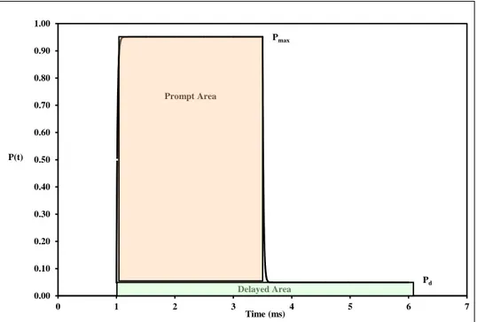
The analogies among these methods can be seen by the following example assuming the validity of the point kinetics approximation. Let us suppose to have a subcritical fast system characterised by the following parameters: k=0.97, βeff=335 pcm (corresponding to a reactivity ρ=-9.2 $), Λ=0.5 μs,
<λ>=0.09 s-1. If we drive the system by a square pulsed neutron source with a frequency 200 Hz and pulse time duration Δτ=2.5 ms, when the delayed background will reach equilibrium we’ll obtain system responses like those shown in Fig. 3.
0.00 0.10 0.20 0.30 0.40 0.50 0.60 0.70 0.80 0.90 1.00 0 1 2 3 4 5 6 7 P(t) Time (ms) Pd Pmax Delayed Area Prompt Area
In the case considered we have a square pulse having a time duration Δτ=2.5ms > |10/αp|, being
|10/αp| ~ 170μs (this requisite for the pulse duration is necessary in order to allow the application of
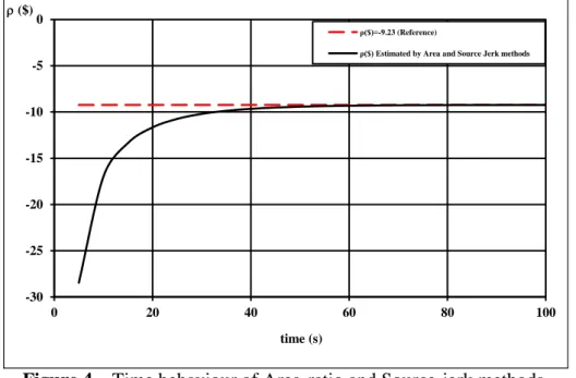
the Source-jerk/Beam-jump methods). It can be seen from Eq. (5) and from Fig. 3 that all the methods make use of the same basic physical quantities to obtain the system reactivity (in dollar units). In particular, for the case considered, the time needed to reach the delayed background equilibrium for all the methods above mentioned is of the order of 10/<λ> (~100s), as shown in Fig. 4. -30 -25 -20 -15 -10 -5 0 0 20 40 60 80 100 ($) time (s) ρ($)=-9.23 (Reference)
ρ($) Estimated by Area and Source Jerk methods
Figure 4 – Time behaviour of Area-ratio and Source-jerk methods.
From the figure it can be seen that all the methods provide (as expected) the same reactivity level at delayed background equilibrium.
As mentioned above, in several practical cases the validity of the point kinetics assumption about the same spatial-energy neutron flux shape for the system driven by only the delayed neutron source and by the external source breaks down, and we have to look for spatial correction factors to apply to the system responses to obtain the reactivity level in dollars units.
4. GODIVA analysis
4.1 GODIVA configurations
GODIVA [14] is an experimental fast reactor originally situated at the Los Alamos National Laboratory (LANL), New Mexico, U.S. GODIVA system is split in three parts and when these are combined they form a critical mass and a nuclear chain reaction is sustained. At the beginning the facility was used to produce bursts of neutrons and gamma rays for irradiating test samples, and finally it became a classical reactor benchmark.
The benchmark considered (identified in the International Handbook of Evaluated Criticality Safety Benchmark Experiments as HEU-MET-FAST-001 [7]) is an unshielded spherical reactor (17.48 cm in diameter) with a fissile metallic mass (density 18.73 g∙cm-3) enriched at 93.71% in U235.
Isotope Density (g/cm3) Number of atoms/cm3 (x10-24)
U235 17.56 4.50∙10-2
U238 0.99 2.50∙10-3
U234 0.19 4.92∙10-4
Table 1 – GODIVA fuel compositions.
Approaching the study of GODIVA by KIN3D module it has been necessary to convert the geometry of the system from spherical to cubic one to allow the analysis of the system by 3D calculations. In fact ERANOS 3D modules, for static and kinetics calculations, do not provide spherical geometries.
The reference critical equivalent cube providing keff ~ 1 (keff = 1.00076) was characterized by a side
equal to 14.75 cm. Afterwards the same system was made subcritical reducing the cube side to 14.5 cm to allow the insertion of the source in the central position to analyse the system kinetic behaviour following pre-determined source transients as previously explained.
To analyse the GODIVA kinetic behaviour in presence of reflectors of different types two different system were taken into account:
1. A copper reflected fissile cube (GODIVA+Copper3). 2. A lead reflected fissile cube (GODIVA+Lead4).
The copper reflector was chosen because of interest for the kinetic behaviour of zero-power copper reflected fast reactors, like TAPIRO reactor at ENEA C.R. Casaccia (see for example [15]), whereas the lead reflector was chosen because of interest for ADS (and GUINEVERE in particular).
The reference critical dimensions for the GODIVA+Copper system are 13 cm as fissile side and 1.7 cm thickness for the copper reflector. The subcritical configuration has the same fissile side and 1.4 cm thickness for the copper reflector. Tab. 2 shows the compositions of the copper reflector for the GODIVA+Copper system.
Isotope Density (g/cm3) Number of atoms/cm3 (x10-24)
Cu63 6.1 5.84∙10-2
Cu65 2.8 2.60∙10-2
Table 2 – Copper compositions for the GODIVA+Copper system.
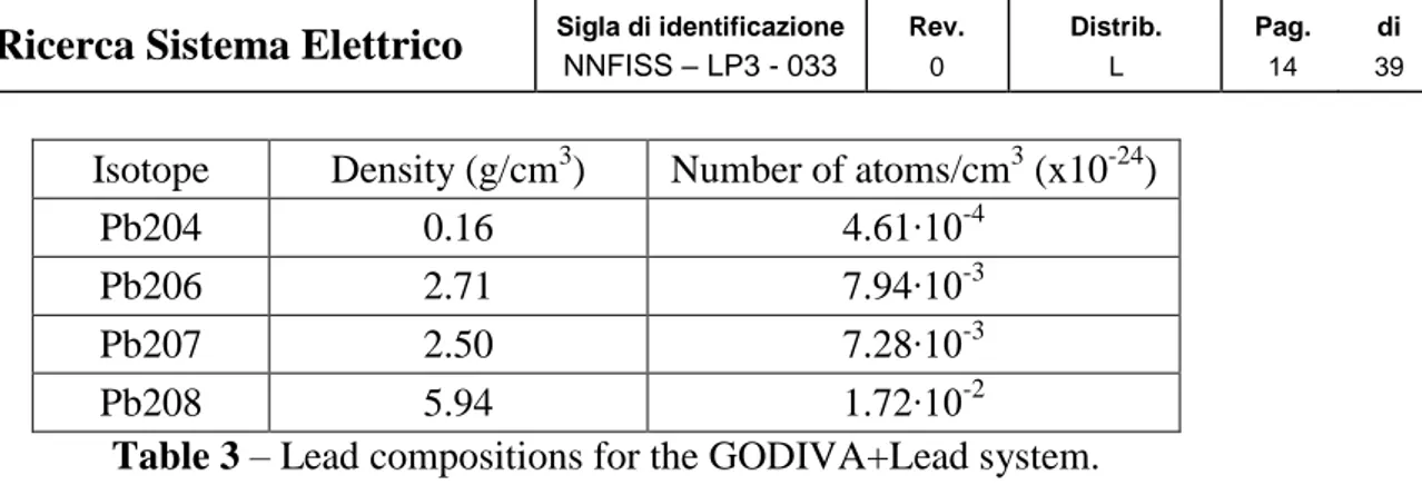
The reference critical dimensions for the GODIVA+Lead system are 13 cm as fissile side (as for the GODIVA+Copper system) and 3.5 cm thickness for the lead reflector. The subcritical configuration has the same fissile side and 2.7 cm thickness for the lead reflector. Tab. 3 shows the compositions of the lead reflector for the GODIVA+Lead system.
3 Natural copper.
Isotope Density (g/cm3) Number of atoms/cm3 (x10-24)
Pb204 0.16 4.61∙10-4
Pb206 2.71 7.94∙10-3
Pb207 2.50 7.28∙10-3
Pb208 5.94 1.72∙10-2
Table 3 – Lead compositions for the GODIVA+Lead system.
A summary for the dimensions of the three different systems (bare, copper reflected and lead reflected), for both critical and subcritical configurations, is shown in Tab. 4 and Tab. 5 respectively.
Critical geometries Fissile side Reflector thickness Total side
GODIVA-bare 14.75 cm \ 14.75 cm
GODIVA+Copper 13 cm 1.7 cm 16.4 cm
GODIVA+Lead 13 cm 3.5 cm 20 cm
Table 4 – Dimensions of the different critical GODIVA geometries analysed.
Subcritical geometries Fissile side Reflector thickness Total side
GODIVA-bare 14.5 cm \ 14. 5 cm
GODIVA+Copper 13 cm 1.4 cm 15.8 cm
GODIVA+Lead 13 cm 2.7 cm 18.4 cm
Table 5 – Dimensions of the different subcritical GODIVA geometries analysed.
4.2 Kinetics calculation specifications
The ECCO module of the ERANOS system was used to produce microscopic and macroscopic cross sections. All the calculations have been performed at 33 energy groups (standard energy grid built-in into ERANOS), shown in Tab. 6 together with the correspondence with the base library at 1968 energy groups. JEFF 3.1 [16] was chosen as reference data library for the analysis. Cross sections were generated using P0 transport approximation.
Upper Energy
(eV) 1968 groups 33 groups
Upper
Energy (eV) 1968 groups 33 groups
1.9640E+07 1 1 5.5308E+03 988 17 1.0000E+07 82 2 3.3546E+03 1048 18 6.0653E+06 142 3 2.0347E+03 1108 19 3.6788E+06 202 4 1.2341E+03 1168 20 2.2313E+06 262 5 7.4852E+02 1228 21 1.3534E+06 322 6 4.5400E+02 1288 22 8.2085E+05 382 7 3.0432E+02 1336 23 4.9787E+05 442 8 1.4863E+02 1422 24 3.0197E+05 502 9 9.1661E+01 1480 25 1.8316E+05 564 10 6.7904E+01 1516 26 1.1109E+05 624 11 4.0169E+01 1579 27 6.7379E+04 686 12 2.2603E+01 1648 28 4.0868E+04 746 13 1.3710E+01 1708 29 2.4788E+04 808 14 8.3153E+00 1768 30 1.5034E+04 868 15 4.0000E+00 1837 31 9.1188E+03 928 16 5.4000E-01 1919 32 1.0000E-01 1952 33
For all three subcritical systems a mono-chromatic 2 MeV energy external source has been inserted at the centre of the geometry inside a 0.5x0.5x0.5 cm3 cube.
Tab. 7 shows delayed neutron data assumed in kinetics calculations, derived from [17]. 33 energy groups delayed neutron spectra, for each delayed neutron family, are the ones built-in into ERANOS (taken from [18]).
Family 1 2 3 4 5 6 Sum
βi 0.00024 0.00137 0.00121 0.00263 0.00084 0.00017 0.00647
Table 7 – 6 groups delayed neutron fractions assumed in GODIVA calculations.
For spatial kinetics calculations two different detector positions (labelled as Det_1 and Det_2 in the plots, being the first nearest to the core centre) were taken into account for all the systems (bare, copper and lead reflector), depending such positions on the system considered. Such detectors have unit cross section and provide as output the total energy integrated flux.
The pattern for the time behaviour of the external source is shown in Fig. 5.
0 0.1 0.2 0.3 0.4 0.5 0.6 0.7 0.8 0.9 1 0 5 10 15 20 25 30 35 S (a.u.) Time (μs) 10 μs 10 μs 10 μs
Time range for the Area-ratio method
1 μs
Figure 5 – GODIVA time behaviour of the external source.
This time behaviour allows to investigate, at one time, the system response for what concerns the application of the three reactivity measurement methods, Slope, Area-ratio and Source-jerk. In fact, considering the order of magnitude of the prompt time constant (|1/αp| < 0.5 μs) for the three
configurations GODIVA bare, copper and lead reflector (results described in detail in the following), this source time behaviour allows to completely charge and discharge prompt neutrons during the source transients, and thus making possible the application of all the three methods. In particular, the following requirements are due to each method for what concerns the time pattern for the external source:
- Slope: none in particular (of course besides the requirement to have sufficient calculated points during the prompt exponential decrease of the response).
- Area-ratio: prompt neutrons must be completely discharged before and after the pulse.
- Source-jerk: as for Area-ratio with the additional requirement that prompt neutrons must be completely charged during the pulse.
Actually there is an additional, important requirement for both Area-ratio and Source-jerk methods: the delayed background must be stable, i.e. in equilibrium with the pulsed neutron source frequency (see preceding sections). Because all the kinetics calculations start at t=0 from the steady initial configuration, the first drop of the source (after 1 μs, see Fig. 5) drives the system response to a delayed background level pertaining to the saturation situation, i.e. in point kinetics to a background level equal to βeff/(βeff-ρ). This works fine for the Source-jerk analysis (also for the drop after 21
μs), whereas for the Area-ratio method we have to renormalize the background level accordingly to time range assumed for the observation of the system response (time range for the application of the method). In our case, we have assumed a time range equal to 20 μs (from 11 μs to 31 μs, Fig. 5), corresponding to a duty cycle 0.5. Consequently in our case all the calculated delayed areas have been multiplied by the factor 0.55.
The calculation steps were the following:
Step 1: adjoint homogeneous flux calculation (outside KIN3D module);
Step 2: direct inhomogeneous flux calculation (by KIN3D module) for the initial steady state6; Step 3: kinetics calculations in approximation point kinetics and direct.
The assumed reference values for ρ, βeff and Λ have been those obtained by KIN3D for the steady
initial configuration at t=0.
4.3 Results
4.3.1 GODIVA Bare
The critical reference configuration (side 14.75 cm, cf. Tab. 4) provided ρ=76 pcm.
For the steady subcritical initial configuration (side 14.5 cm, cf. Tab. 5) at t=0, the reference values for ρ, βeff and Λ obtained by KIN3D are ρ=-1403 pcm corresponding to ρ($)= -2.13 $ with βeff=658
pcm, and Λ=6.53∙10-9 s providing |αp| ~ 3.16∙106 s-1 (|1/αp| ~ 0.3 μs).
The position of the detectors (kinetics direct spatial calculation) for the subcritical GODIVA Bare configuration is shown in Fig. 6.
5 For the Slope technique, denoting DC as Duty Cycle, in point kinetics formalism we have for the generic time t:
t eff eff h eff eff p e DC P DC t P ) (
where Ph is the flux amplitude before the source shutdown.
6
Some fictitious transients starting at t=0 have been observed (probably because incoherence on the source level normalisation) when providing from the outside to KIN3D the inhomogeneous fluxes of the steady initial configuration at t=0.
Figure 6 – GODIVA Bare. Detectors position (in blue source position).
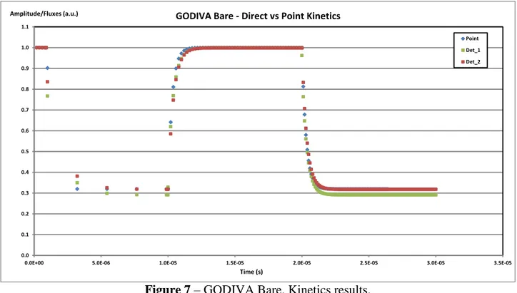
Fig. 7 shows the system response following the source transient in Fig. 5.
0.0 0.1 0.2 0.3 0.4 0.5 0.6 0.7 0.8 0.9 1.0 1.1
0.0E+00 5.0E-06 1.0E-05 1.5E-05 2.0E-05 2.5E-05 3.0E-05 3.5E-05 Point Det_1 Det_2
Time (s)
Amplitude/Fluxes (a.u.) GODIVA Bare - Direct vs Point Kinetics
Figure 7 – GODIVA Bare. Kinetics results.
It’s important to highlight that KIN3D results are normalized to unit, separately for each detector, for t=0. This implies a misleading interpretation, at first sight, of the relative behaviour of the different responses of detectors placed in different system positions. As an example, Fig. 8 shows the total (energy integrated) flux profiles, obtained by the inhomogeneous flux calculation for the initial steady state at t=0, in correspondence of the two detectors Det_1 and Det_2.
0.0E+00 5.0E-02 1.0E-01 1.5E-01 2.0E-01 2.5E-01 -8 -7 -6 -5 -4 -3 -2 -1 0 1 2 3 4 5 6 7 8
Flux (a.u.) GODIVA Bare - Initial steady state
Distance from the source (cm)
Det_1
Det_2
Figure 8 – GODIVA Bare. Flux at t=0 and detectors position.
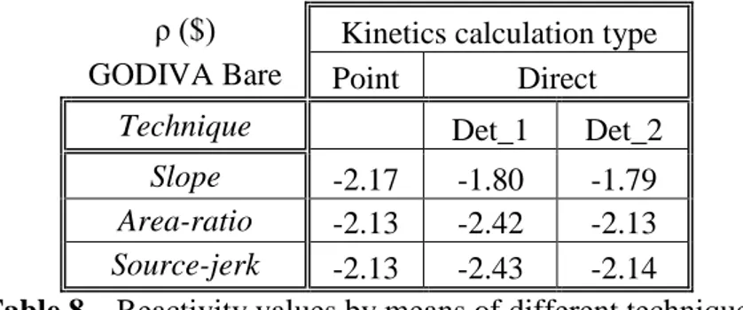
Tab. 8 shows the reactivity values inferred by means of different measurement techniques from the results in Fig. 7.
ρ ($) Kinetics calculation type
GODIVA Bare Point Direct
Technique Det_1 Det_2
Slope -2.17 -1.80 -1.79
Area-ratio -2.13 -2.42 -2.13
Source-jerk -2.13 -2.43 -2.14
Table 8 – Reactivity values by means of different techniques.
Reference reactivity ρ($)= -2.13 $. It can be seen that:
In point kinetics calculation the slope technique does not return exactly (as expected) the reference reactivity value. On the contrary, Area-ratio and Source-jerk techniques return exactly the reference reactivity value.
Both detectors in spatial direct calculations provide the same slope (similar reactivity values between Det 1 and Det 2) but do not provide the reference reactivity value.
Det 2 (farther from the source) provides good results by both Area-ratio and Source-jerk techniques, whereas Det 1 provides similar results by both Area-ratio and Source-jerk techniques but different (less than about 30 cents in any case) from the reference reactivity value.
In synthesis, for the GODIVA Bare system KIN3D results show that spatial effects are present. In particular the slope technique is not reliable to evaluate the system reactivity whereas Area-ratio and Source-jerk techniques provide reliable results only far from the source.
4.3.2 GODIVA+Copper
For the steady subcritical initial configuration (side 15.8 cm, cf. Tab. 5) at t=0, the reference values for ρ, βeff and Λ obtained by KIN3D are ρ=-1229 pcm corresponding to ρ($)= -1.83 $ with βeff=671
pcm, and Λ=7.45∙10-9
s providing |αp| ~ 2.55∙106 s-1 (|1/αp| ~ 0.4 μs).
The position of the detectors (kinetics direct spatial calculation) for the subcritical GODIVA+Copper configuration is shown in Fig. 9.
Figure 9 – GODIVA+Copper. Detectors position (in blue source position).
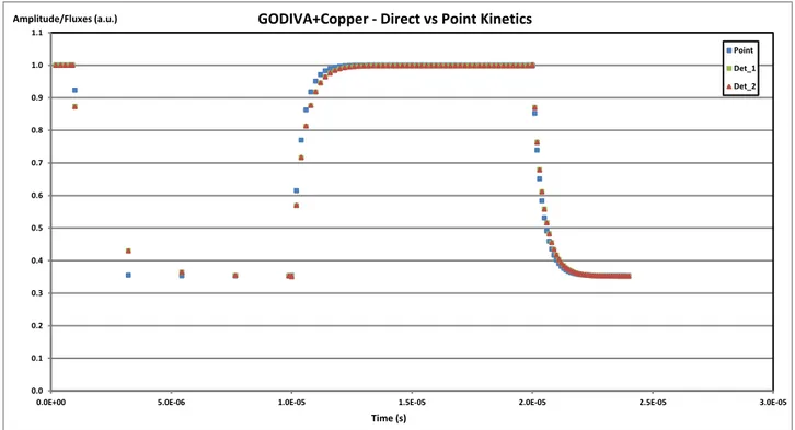
Fig. 10 shows the system response following the source transient in Fig. 5.
0.0 0.1 0.2 0.3 0.4 0.5 0.6 0.7 0.8 0.9 1.0 1.1
0.0E+00 5.0E-06 1.0E-05 1.5E-05 2.0E-05 2.5E-05 3.0E-05
Point Det_1 Det_2
Time (s)
GODIVA+Copper - Direct vs Point Kinetics
Amplitude/Fluxes (a.u.)
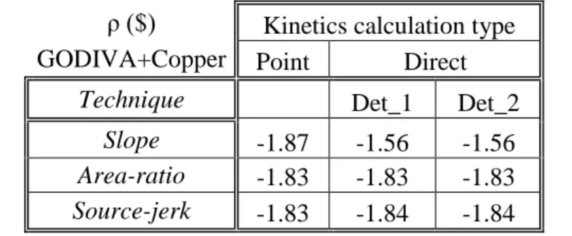
Tab. 9 shows the reactivity values inferred by means of different measurement techniques from the results in Fig. 10.
ρ ($) Kinetics calculation type
GODIVA+Copper Point Direct
Technique Det_1 Det_2
Slope -1.87 -1.56 -1.56
Area-ratio -1.83 -1.83 -1.83
Source-jerk -1.83 -1.84 -1.84
Table 9 – Reactivity values by means of different techniques.
Reference reactivity ρ($)= -1.83 $. It can be seen that:
In point kinetics calculation the slope technique does not return exactly (as expected) the reference reactivity value. On the contrary, Area-ratio and Source-jerk techniques return exactly the reference reactivity value.
Both detectors in spatial direct calculations provide the same slope (similar reactivity values between Det 1 and Det 2) but do not provide the reference reactivity value.
Both detectors provide good results by both Area-ratio and Source-jerk techniques.
In synthesis, for the GODIVA+Copper system KIN3D results show that spatial effects are present only for the slope technique, which is not reliable to evaluate the system reactivity. On the contrary Area-ratio and Source-jerk techniques provide reliable results for the detector positions considered (in any case both far from the source unlike GODIVA Bare case where a detector was near the source, see Figs. 6 and 9).
4.3.3 GODIVA+Lead
The critical reference configuration (side 20.0 cm, cf. Tab. 4) provided ρ=-599 pcm.
For the steady subcritical initial configuration (side 18.4 cm, cf. Tab. 5) at t=0, the reference values for ρ, βeff and Λ obtained by KIN3D are ρ=-1229 pcm corresponding to ρ($)= -3.08 $ with βeff=666
pcm, and Λ=7.66∙10-9
s providing |αp| ~ 3.54∙106 s-1 (|1/αp| ~ 0.3 μs).
The position of the detectors (kinetics direct spatial calculation) for the subcritical GODIVA+Lead configuration is shown in Fig. 11.
Figure 11 – GODIVA+Lead. Detectors position (in blue source position).
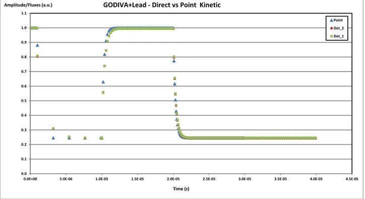
Fig. 12 shows the system response following the source transient in Fig. 5.
0.0 0.1 0.2 0.3 0.4 0.5 0.6 0.7 0.8 0.9 1.0 1.1
0.0E+00 5.0E-06 1.0E-05 1.5E-05 2.0E-05 2.5E-05 3.0E-05 3.5E-05 4.0E-05 4.5E-05 Point Det_2 Det_1
Time (s)
GODIVA+Lead - Direct vs Point Kinetic
Amplitude/Fluxes (a.u.)
Figure 12 – GODIVA+Lead. Kinetics results.
Tab. 10 shows the reactivity values inferred by means of different measurement techniques from the results in Fig. 12.
ρ ($) Kinetics calculation type
GODIVA+Lead Point Direct
Technique Det_1 Det_2
Slope -3.08 -2.47 -2.47
Area-ratio -3.08 -3.05 -3.08
Source-jerk -3.08 -3.08 -3.12
Table 10 – Reactivity values by means of different techniques.
Reference reactivity ρ($)= -3.08 $. It can be seen that:
Both detectors in spatial direct calculations provide the same slope (similar reactivity values between Det 1 and Det 2) but do not provide the reference reactivity value.
Both detectors provide good results by both Area-ratio and Source-jerk techniques.
In synthesis, for the GODIVA+Lead system KIN3D results show that spatial effects are present only for the slope technique, which is not reliable to evaluate the system reactivity. On the contrary Area-ratio and Source-jerk techniques provide reliable results for the detector positions considered (same considerations as for GODIVA+Copper).
5. GUINEVERE analysis
5.1 Generalities
On the basis of the outcome of the MUSE experimental campaign [19], two points were left open for significant improvement:
1. To validate the methodology for reactivity monitoring by a continuous accelerator beam (not available in the MUSE programme).
2. To have representative conditions of a lead-cooled ADS by a lead matrix core (requirement only partially satisfied by the MUSE programme).
To meet the above issues, SCK•CEN has proposed to use a modified lay-out of the VENUS critical facility located at its Mol-site and to couple it to a deuteron accelerator (GENEPI type used in MUSE) working in current mode and delivering 14 MeV neutrons by bombardment of deuterons on a tritium-target: on these premises the GUINEVERE-project (Generator of Uninterrupted Intense NEutrons at the lead VEnus REactor) was launched. The GUINEVERE experimental program [5], launched in 2007 as European project included in the Integrated Project (IP) EUROTRANS of the Sixth EU Framework Programme, will flow into the FREYA project [6], started on March 2011, of the Seventh EU Framework Programme.
Figure 13 – First lay-out of a GUINEVERE core arrangement
This configuration consists of 92 fuel assemblies (86 fuel assemblies + 6 safety rods with fuel follower) of about 60 cm active length. Each fuel assembly contains nine fuel elements with in between lead rodlets as can be seen from Fig. 13 on the right (taken from [21]). The square core has a side of about 1 m and it is surrounded by a cylindrical lead reflector (about 30 cm thickness in the radial direction and about 40 cm height for the upper and lower part). In Fig. 13 the central hole for the accelerator beam tube and the target material is shown.
The fuel rodlets are made of metallic Uranium 30 wt.% enriched in U-235, with a diameter of 1.27 cm and a height of 20.32 cm. Three of them are piled up in a 5×5 lattice filled with lead blocks and fuel rodlets, as shown in Fig. 13, in order to obtain an active fuel height of 60.96 cm.
As reference core arrangement was taken into account the nominal critical start-up configuration (named CR0), shown in Fig. 14, characterized by 88 fuel assemblies (82 fuel assemblies + 6 safety rods with fuel follower), and with the core fully loaded with fuel assemblies (no central hole for the accelerator beam tube).
As shown in Fig. 15, where a general schematic axial lay-out of the reactor is given, the cylindrical core has the following dimensions: diameter D = 160.8 cm and effective height7 H = 161.7 cm (D/H = ≈ 1, practically a square cylinder).
0.789 0.75 31.98 31.98 21 Void Void 5 66.36 5 96.84=8.07×12 40.3 5 19.29 Core lattice active lenght
Radial upper grid (AISI 304) Radial upper grid
(AISI 304)
Radial lower grid (AISI 304) 40
Reactor vessel Radial lower grid
(AISI 304)
Radial reflector (lead)
Radial bottom grid (AISI 304)
Radial reflector (lead) Radial reflector (lead) Radial reflector (lead) Air Radial reflector (lead) Radial reflector (lead) 60.96
Figure 15 – Schematic axial lay-out of the GUINEVERE reactor (dimensions in cm not in scale).
The core lattice consists of 12×12 square assemblies, each one 8 cm side, with a 0.7 mm inter-assemblies air gap (see Fig. 14). There are 82 fuel inter-assemblies + 6 safety rods with fuel follower. The remaining assemblies are 2 control rods and lead assemblies. The core lattice has an external square AISI 304 sheet (3 cm thickness), height 76.36 cm, having an air gap with the inner assemblies equal to 2.65 mm, as shown in Fig. 15.
As before mentioned, all along the core active length each fuel assembly and safety rod is structured in a 5×5 lattice (see Fig. 16) containing 9 cylindrical fuel rodlets (each one made of 3 sub-cylinders, with radius 0.63 cm and height 20.3 cm, stacked on top of each other), 12 square (1.27 cm side) lead rodlets with SS 304 L cladding (each one made of 6 lead SS 304 L cladded parallelepipeds, with side 1.27 cm and height 10.16 cm, stacked on top of each other), and 4 square (1.27 cm side, mono-block) lead rodlets without cladding.
19.29 60.96
Cladded lead rodlet
1.27 Lead rodlet Fuel Nickel Lead AISI 304 1.27 Fuel rodlet 60.96 1.27 8.07 40 SS 304 L Air 21.789 5 7.7 40.3 7.7 Fuel assembly Safety rod (only active length)
Figure 16 – Sketch of fuel assemblies (dimensions in cm not in scale).
The uranium in the fuel rodlets is 30% (weight) enriched in U235. Each fuel assembly has a 3 layers AISI 304 – lead – AISI 304 (overall thickness 8.25 mm) sheet.
The absorbing part of the 6 safety rods and 2 control rods, placed above the active core, has an height equal to 60.9 cm (practically equal to the core active length), and contains a square (7 cm side) element containing 5.8 kg of B4C with a SS 304 L cladding (see Fig. 17).
0.6 0.6 0.289 0.289 8.07 60.9 68.66 8.07 60.9 60.96 7.7 B4C 2 Control rod 7.7 Safety rod 70.29 64.59 19.29 Lead AISI 304 SS 304 L Air 7.7 40.3 5 8.07 Lead assembly 40 7.7 60.96 21.789
Figure 17 – Sketch of safety/control rods and lead assemblies (dimensions in cm not in scale).
5.2 ERANOS calculation model set-up
5.2.1 Cross section sets generation by the ECCO module
The ECCO module of the ERANOS system was used to produce microscopic and macroscopic cross sections. All the calculations have been performed at 33 energy groups shown (Tab. 6). JEFF 3.1 was chosen as reference data library for the analysis. Cross sections were generated using P0
transport approximation.
As previously mentioned, all along the core active length each fuel assembly and safety rod is structured in a 5×5 lattice (see Fig. 18) containing 9 cylindrical fuel rodlets, 12 square lead rodlets with SS 304 L cladding and 4 square lead rodlets without cladding (dark grey squares in Fig. 18). Cross sections for this part of both fuel assemblies and safety rods were obtained by ECCO (bi-dimensional) heterogeneous cell calculations.
Figure 18 – Fuel assembly (not scale drawing, dimensions in cm).
Figure 19 – ECCO model of the active part of both fuel assemblies and safety rods
(not scale drawing, dimensions in cm).
For the control and safety rods cell calculations, two zones have been considered: the external structural box, made of SS and air, and the absorber zone made of B4C, treated separately. In Figs.
20-21 horizontal sections of control and safety rods are shown.
Figure 21 - ECCO control and safety rod absorbing part and box model.
The active part of the safety rod is similar but not identical to the active part of the fuel assembly. In Fig. 22 the corresponding ECCO model is shown.
Figure 22 – Safety rod active part - ECCO model.
The central channel for the beam tube is modelled as a squared channel (size 16.14×16.14 cm2) with a central hole (6.3×6.3 cm2) going from the core bottom up to the top of the reactor (Fig. 23).
5.2.2 Reactor modelling
The cylindrical reflector of the GUINEVERE reactor needs to be modelled in rectangular XYZ geometry. To this end, two basic approaches can be considered: a first one straightforward approach is to model the circular plane section of the cylinder, having a radius r and height h, by a square having the same area (and thus preserving mass), i.e. having a side ℓ= r∙√π. In such a way the neutrons leakage surface from the parallelepiped reflector is 4ℓ∙h = 4r∙√π∙h against the cylindrical reference value 2π∙r∙h. Thus, following this approach the leakage from the reflector is overestimated by a factor 2/√π ≈ 1.13. A second refined approach is to approximate the circular plane section of the cylinder by a rectilinear polygon having the same area of the circular section and a pre-determined number of edges. In our case it was chosen to have a 32 edges polygon as shown in Fig. 24. -100.00 -80.00 -60.00 -40.00 -20.00 0.00 20.00 40.00 60.00 80.00 100.00 -100.00 -80.00 -60.00 -40.00 -20.00 0.00 20.00 40.00 60.00 80.00 100.00 x0=r
Figure 24 – 32 edges polygon approximating the circular plane section of the cylindrical reflector.
In particular, by means of a simple algorithm set up for the need, the circle area was divided by 32 equi-area sectors and the polygon was built accordingly to the initial constraint x0=r (see Fig. 24,
where are shown 8 equi-area sectors for one quadrant). The green piecewise-linear curve in Fig. 24, obtained by joining two by two the different edges of the polygon, shows the effective leakage
perimeter from the rectilinear polygon. This quantity tends to 2πr for n→∞, with n number of
edges8. In our case, modelling the cylindrical reflector by a 32 sectors polygon the leakage perimeter is overestimated by a factor ≈ 1.03 (leakage factor, to be compared with the above mentioned value ≈ 1.13 corresponding to a simple square having the same area of the circular plane section of the cylinder). At last, a fine “handmade” tuning of the polygon edges was performed, always with the constraint to preserve the same circle area and the leakage factor ≈ 1.03, in order to match with some mesh constraints in the XYZ reactor model. Fig. 25 shows the final reflector modelling and a comparison with the corresponding circle shape.
8 Vice versa, the perimeter of the rectilinear polygon tends to 8r, as can be inferred geometrically from the figure, for
80.0 96.14 112.28 120.35 131.65 140.65 148.65 154.65 160.00 0.0 5.35 11.35 19.35 28.35 38.815 47.72 63.86 0.0 4.87 9.19 15.31 24.43 31.58 47.72 80.0 104.21 112.28 128.42 135.57 144.69 150.81 155.13 160.0 1 2 3 4 5 8 10 12 14 16 18 19 23 24 25 26 27 1 23 4 5 7 9 10 20 21 23 25 26 27 28 29 55.79 15
Figure 25 - GUINEVERE reflector modelling.
The subcritical configuration (without the four central assemblies respect to the nominal critical configuration) analysed by KIN3D is shown in Fig. 26.
5.3 Kinetics calculation specifications
All the kinetics calculation, unless otherwise specified, were performed with the same specifications as for GODIVA analysis.
A mono-chromatic 14 MeV energy external source has been inserted at the centre of the geometry inside a 8.07×8.07×12.192 cm3 parallelepiped.
Tab. 11 shows delayed neutron data assumed in kinetics calculations9.
Family 1 2 3 4 5 6 Sum
βi 0.00025 0.00147 0.00136 0.003 0.00109 0.00026 0.00743
Table 11 – 6 groups delayed neutron fractions assumed in GUINEVERE calculations.
For spatial kinetics calculations three different detector positions (labelled as Det_1, Det_2 and Det_3 in the plots) were taken into account. As in GODIVA case, such detectors have unit cross section and provide as output the total energy integrated flux. The position of the detectors is shown in Fig. 27.
Figure 27 – GUINEVERE. Detectors position.
9 Considering the mixture U235 (30%) – U238 (70%) relative to the GUINEVERE fuel, average β
i were obtained by
the formula (written in standard notation, with m isotope index, g energy group index and <...>V volume integral):
g V m g f m g g m V g m g f m g g m i m i
r r r r ' ) ( ' , ) ( ' ' ' ) ( ' , ) ( ' ' ) ( ˆ ˆ .It’s important to recall that KIN3D results are normalized to unit, separately for each detector, for t=0. Fig. 28 shows the total (energy integrated) flux profiles, obtained by the inhomogeneous flux calculation for the initial steady state at t=0, in correspondence of the three detectors Det_1, Det_2 and Det_3. 0.0E+00 2.0E+00 4.0E+00 6.0E+00 8.0E+00 1.0E+01 1.2E+01 1.4E+01 1.6E+01 -80 -60 -40 -20 0 20 40 60 80
GUINEVERE - Initial steady state Flux (a.u.)
Distance from the source centerline - Y direction (cm)
DET_1
DET_3
DET_2
Figure 28 – GUINEVERE. Flux at t=0 and detectors position10.
The pattern for the time behaviour of the external source is shown in Fig. 29.
0 0.1 0.2 0.3 0.4 0.5 0.6 0.7 0.8 0.9 1 0 50 100 150 200 250 S (a.u.) Time (μs) 100 μs 19 μs 90 μs
Time range for the Area-ratio method
1 μs
Figure 29 – GUINEVERE. Time behaviour of the external source.
Also in this case the time behaviour allows investigating, at one time, the system response for what concerns the application of the three reactivity measurement methods Slope, Area-ratio and Source-jerk. In fact, considering the order of magnitude of the prompt time constant (|1/αp| ~ 10 μs) for the
10 Flux traverses are displaced 4.035 cm respect to the source centerline (see Fig. 27). This explains the absence of the
GUINEVERE subcritical configuration, this source time behaviour allows discharging completely prompt neutrons during the first drop of the source after 1 μs (we recall that the first drop of the source brings the system response to a delayed background level pertaining to the saturation situation). This allows the Source-jerk (and Slope) method analysis. Vice-versa during the time interval starting at 101 μs, and lasting 19 μs, prompt neutrons are not completely charged during the pulse. This allows in any case the application of the Area-ratio method taking care with regard to the renormalization of the background level accordingly to time range assumed for the observation of the system response (see GODIVA sections). In our case, we have assumed a time range equal to 109 μs (from 101 μs to 210 μs, Fig. 29), corresponding to a duty cycle 19/109. Consequently in our case all the calculated delayed areas have been multiplied by the factor 19/109.
5.4 Results
For the steady subcritical initial configuration at t=0, the reference values for ρ, βeff and Λ obtained
by KIN3D are ρ=-4042 pcm corresponding to ρ($)= -5.58 $ with βeff=725 pcm, and Λ=4.52∙10-7 s
providing |αp| ~ 1.05∙105 s-1 (|1/αp| ~ 9.5 μs).
Fig. 30 shows the system response following the source transient in Fig. 29.
0.0 0.1 0.2 0.3 0.4 0.5 0.6 0.7 0.8 0.9 1.0 1.1
0.0E+00 2.0E-05 4.0E-05 6.0E-05 8.0E-05 1.0E-04 1.2E-04 1.4E-04 1.6E-04 1.8E-04 2.0E-04 2.2E-04 2.4E-04
GUINEVERE - Direct vs Point Kinetics
Point Det_1 Det_2 Det_3 Time (s) Amplitude/Fluxes (a.u.) Source-jerk Area-ratio Slope
No saturation on prompt neutrons
Slope
βeff/(βeff-ρ)
Figure 30 – GUINEVERE. Kinetics results.
In Fig. 30 are evidenced the various time zones of the system responses where the different reactivity measurement techniques have been applied. As mentioned in the preceding sections, because all the kinetics calculations start at t=0 from the steady initial configuration, the first drop of the source (after 1 μs, see Fig. 29) drives the system response to a delayed background level pertaining to the saturation situation, i.e. in point kinetics to a background equal to βeff/(βeff-ρ). This
allows applying the Source-jerk technique directly after the first drop of the source, and this is very important for the GUINEVERE because the behaviour of the flux/amplitude after the 19 μs pulse
does not show saturation on prompt neutrons, unlike GODIVA case, i.e. it’s not possible to apply
the Source-jerk approach in correspondence of the neutron pulse (Fig. 30).
Tab. 12 shows the reactivity values inferred by means of different measurement techniques from the results in Fig. 29.
ρ ($) Kinetics calculation type
GUINEVERE Point Direct
Technique Det_1 Det_2 Det_3
Slope -5.58 -5.30 -5.22 -4.96
Area-ratio -5.58 -5.67 -5.34 -5.29
Source-jerk -5.57 -5.60 -5.28 -5.24
Table 12 – ERANOS/KIN3D Reactivity values by means of different techniques.
Reference reactivity ρ($)= -5.58 $. It can be seen that:
Detectors in spatial direct calculations provide (slightly) different slope, corresponding to a maximum difference respect to the reference reactivity less than about 60 cents.
Both Area-ratio and Source-jerk techniques provide reasonable results for all the detectors, corresponding to a maximum difference respect to the reference reactivity less than about 35 cents.
In synthesis, for the GUINEVERE system KIN3D results show that spatial effects are present but do not strongly influence the observed reactivity, depending on the position and on the measurement technique, respect to the reference one.
To better appreciate the order of magnitude of the spatial effects when observing the slopes of the different detectors responses after the shutdown(s) of the source, Fig. 31 shows such the responses up to 60 microseconds after the source shutdown.
0.0 0.1 0.2 0.3 0.4 0.5 0.6 0.7 0.8 0 10 20 30 40 50 60 Det_1 Det_2 Det_3 Flux (a.u.) Time (μs)
ERANOS - Direct Kinetics - Detectors 1-2-3
5.5 ERANOS/KIN3D-MCNPX results comparison.
The same GUINEVERE configuration shown in Fig. 26 has been analysed through Monte Carlo calculations by MCNPX [22]. As nuclear data library was selected JEFF 3.1 [23]. Delayed neutron data were derived from [18] (8 families assumed in calculations).
Concerning the external source an isotropic point mono-chromatic 14 MeV energy external source has been inserted at the centre of the geometry. A Dirac time-shape was chosen as pulse time profile of the external neutron source.
The same three different detector positions (Det_1, Det_2 and Det_3, see Fig. 27) were taken into account, providing such detectors the total energy integrated flux (as in the ERANOS/KIN3D calculations).
For the steady subcritical initial configuration at t=0, the reference values for ρ, βeff and Λ obtained
by MCNPX are ρ=-3310 pcm corresponding to ρ($)= -4.55 $ with βeff=727 pcm, and Λ=4.68∙10-7 s
providing |αp| ~ 8.62∙104 s-1 (|1/αp| ~ 11.6 μs). The Λ value was derived from [24, 25].
Taking into consideration the reactivity difference between ERANOS/KIN3D and MCNPX results (ERANOS result is about 700 pcm lower respect to MCNPX one), only for sake of completeness Tab. 13 shows the reactivity values inferred by means of different measurement techniques from MCNPX results.
ρ ($) GUINEVERE
Technique Det_1 Det_2 Det_3
Slope -4.30 -4.19 -4.09
Area-ratio -4.50 -4.27 -4.27
Source-jerk -5.20 -5.14 -4.29
Table 13 – MCNPX reactivity values by means of different techniques.
Reference reactivity ρ($)= -4.55 $.
It can be noticed that, in spite of the difference in reactivity level between ERANOS/KIN3D and MCNPX results, the general trend of the different reactivity measurement techniques shown in Tab. 12 and Tab. 13 exhibits some analogies. This can be seen more clearly from Tab. 14, where the differences respect to the reference reactivity for both codes and for each measurement technique are shown.
ERANOS/KIN3D MCNPX
Technique Det_1 Det_2 Det_3 Technique Det_1 Det_2 Det_3
Slope 0.28 0.36 0.62 Slope 0.25 0.36 0.46
Area-ratio -0.09 0.24 0.29 Area-ratio 0.05 0.28 0.28
Source-jerk -0.02 0.30 0.34 Source-jerk -0.65 -0.59 0.26
Table 14 – ERANOS/KIN3D-MCNPX reactivity values by means of different techniques.
![Tab. 7 shows delayed neutron data assumed in kinetics calculations, derived from [17]](https://thumb-eu.123doks.com/thumbv2/123dokorg/5622621.68611/15.892.87.813.514.902/tab-shows-delayed-neutron-assumed-kinetics-calculations-derived.webp)