A procedure for the optimal management of medium-voltage AC networks with distributed generation and storage devices

Procedia - Social and Behavioral Sciences 108 ( 2014 ) 164 – 186

1877-0428 © 2013 The Authors. Published by Elsevier Ltd. Open access under CC BY-NC-ND license. Selection and peer-review under responsibility of AIRO.

doi: 10.1016/j.sbspro.2013.12.829

ScienceDirect

AIRO Winter 2013

A procedure for the optimal management of medium-voltage AC

networks with distributed generation and storage devices

Alessandro Bosisio

, Diana Moneta

, Maria Teresa Vespucci

*, Stefano Zigrino

a_{Department of Energy, Politecnico di Milano,via La Masa 34, Milano 20165, Italy} b_{Ricerca sul Sistema Energetico SpA, Via Rubattino 54, Milano 20134, Italy} c

Department of Management, Economics and Quantitative Methods,University of Bergamo, via dei Caniana 2, Bergamo 24127, Italy

Abstract

A medium-voltage AC network with distributed generation and storage devices is considered for which set points are assigned in each time period of a given time horizon. A set point in a time period is defined by modules and phases of voltages in all nodes, active and reactive powers, on load tap changer and variable loads. When some parameters vary, in order to restore feasibility new set points need to be determined so as to minimize the variations with respect to the initial ones. This can be done by minimizing distributor’s redispatching costs, which are modeled by means of binary variables, while satisfying service security requirements and ensuring service quality, which are represented by nonlinear constraints, such as the nodal balance of active and reactive power and the current transits on lines and transformers for security. Storage devices are modeled by means of constraints that relate adjacent time periods. A two-step solution procedure is proposed, which is based on decoupling active and reactive variables: in the first step a MILP model determines the active power production and the use of storage devices that minimize redispatching costs over all time periods in the time horizon; in the second step, given the optimal active power production computed in the first step, reactive variables in each time period are computed by solving a nonlinear programming model.

© 2013 The Authors. Published by Elsevier Ltd. Selection and peer-review under responsibility of AIRO.

Keywords: distributed generation; voltage control; electric storage; optimization.

1. Introduction

Distribution networks in current power systems are designed and operated as the final stage in the delivery of electricity: electric power is mainly generated by large power plants connected to the high voltage network, by

* Corresponding author. Tel.: +39-035-2052071; fax: .: +39-035-2052077.

E-mail address: maria-teresa.vespucci@unibg.it

© 2013 The Authors. Published by Elsevier Ltd. Open access under CC BY-NC-ND license. Selection and peer-review under responsibility of AIRO.

which power is transmitted to medium voltage distribution networks. In line with the environmental targets set up by EU for 2020, distribution networks are going to change their current role, in order to allow penetration of Distributed Generation (DG), i.e. power plants directly connected to distribution networks, such as micro cogeneration units and generators using renewable energy sources (wind power plants, photovoltaic plants). Distribution networks will have to host both dispatchable power plants, for which production plans are determined by the owner one day ahead on the basis of load and price forecast, and non dispatchable power plants, for which only production forecasts are available in advance, on the basis of weather forecast (wind speed, solar radiation). Due to partial unpredictability of both load and power generation from non dispatchable power plants, unbalance between generation and load is very likely to occur. The Distribution System Operator (DSO) will be in charge of operating the distribution network so as to guarantee technical feasibility. For compensating unbalances, the DSO can rely on “internal” regulation resources (i.e. directly operated by the DSO), such as On- Load Tap Changers (OLTC) and storage units, and on “external” regulation resources, such as active and reactive power injection/absorption from controllable resources.

Costs of internal resources and rewards for controllable generators (inverter-based or with a synchronous interface) have to be associated to their use: active power exchanges with the HV network can be evaluated at the market price of electricity; the cost of using storage devices may represent device deterioration, taking into account power losses; power producers have to be compensated by the DSO for modifying or interrupting power generation: the following costs are proposed by the Italian Energy Authority (AEEG)

• a fixed cost for interrupting active power generation of dispatchable and non-dispatchable generators;

• a fixed cost for modifying planned active power generation of dispatchable generators;

• a cost per unit of increased/decreased power output.

The DSO problem consists of determining the best control action to take when unbalance between load and generation occurs, i.e. when realized values of load and of non dispatchable generation differ from the forecasts used in the planning phase. The changes to be requested to controllable resources are determined so as to minimize the cost of the DSO control action, while satisfying technical constraints. The DSO problem can be represented by a multi-period Mixed Integer Non Linear Programming (MINLP) model, where integrality is due to the binary variables for modeling fixed costs and nonlinearity pertains to the constraints of the Optimal Power Flow problem. The time period, or planning horizon, under consideration is discretized in time units (e.g., one day divided in 24 hours or in 96 quarters of hour) and intertemporal energy balance constraints are introduced to model storage units. Distribution networks with a large number of nodes and lines give rise to large dimensional MINLP models, which in turn require large computational effort for their solution. Therefore in this work we propose a procedure for the optimal operation of distribution networks based on decoupling integrality and nonlinearity. The procedure consists of two steps: the first one is based on a Mixed Integer Linear Programming

(MILP) model that determines, for all time units of the period under consideration, the active power of dispatchable generators and the use of storage devices (OPF-CC) so as to minimize the cost of the DSO control action over all time units; the second step is based on a Non Linear Programming (NLP) model for every single time unit, which determines, starting from the optimal active power production computed in Step 1, active and reactive power of dispatchable generators so as to minimize active and reactive power production costs, while satisfying security requirements (current) and ensuring service quality (voltages).

The paper is organized as follows. In Section 2 the models used in the procedure are presented. Results of numerical experiments are discussed in Section 3. Conclusions and further research is discussed in Section 4.

2. The two-step procedure for the optimal operation of distribution networks

In the planning phase active and reactive power production of controllable generators, modules and phases of voltages in all network nodes, current flows on lines and the usage of electric storages are determined on the basis of forecasted values of loads and of non-dispatchable generations. When realized values differ from the forecasted ones, i.e. when unbalance between load and generation occurs, for each time unit it is necessary to determine how the previously determined values (active and reactive power productions, modules and phases of voltages, current flows, energy rates to and from electric storages) have to be modified, in order to satisfy the so called Optimal Power Flow (OPF) constraints, which ensure security and power quality. Feasible solutions to this problem are defined by a set of nonlinear constraints, the dimension of which depends on the number of network nodes and lines and on the number of time units to be considered simultaneously for modeling storage units. Among all feasible solutions the DSO wishes to find one of minimum cost, as modifications to previously planned solutions have to be paid for. Indeed, costs are accounted for representing storage device deterioration and active power exchanges with the HV network, while the AEEG is proposing a compensation scheme, based both on cost-per-unit and on fixed costs, for power producers requested to modify or interrupt their scheduled power generation. For the resulting MINLP optimal network operation model we propose a two-step solution procedure based on decoupling integrality and nonlinearity:

1. the first step, based on a MILP model, determines, for all time units of the period under consideration, the variations of active power production of dispatchable generators and of the use of storage devices, so as to minimize the cost of the DSO control action over all time units;

2. the second step, based on a NLP model, determines, starting from the optimal active power production computed in Step 1, active and reactive power production of dispatchable generators, modules and phases of voltages in all network nodes, current flows on lines and the usage of electric storages, so as to minimize active and reactive power production costs, while satisfying security requirements and ensuring service quality.

In the following subsections we describe in detail the MILP model and we briefly sketch the main elements of the NLP model used, based on Garzillo, Innorta, & Ricci (1998).

2.1. Step 1: the MILP model for the optimal active power dispatch

In order to introduce the MILP model used in Step 1 of the procedure, the following symbols are defined.

Sets

I set of nodes, indexed by i

K set of lines, indexed by k

G set of power generators, indexed by g

B set of storage units, indexed by b

T set of time units, indexed by t, in which the period under consideration is divided.

Moreover, GND denotes the subset of non dispatchable generators, GD denotes the subset of dispatchable

generators with non interruptible production and GDS denotes the subset of dispatchable generators with

interruptible production.

Parameters

dt [h] duration of time unit

[€] fixed cost for interrupting production of generator g

[€] fixed cost for modifying scheduled production of generator g

[€/MWh] unitary cost for increasing production of generator g

[€/MWh] unitary cost for decreasing production of generator g

[€/MWh] unitary cost of input in storage unit b

[€/MWh] unitary cost of output from storage unit b

[MW] power output of dispatchable generator g in period t

[MW] maximum power output of dispatchable generator g

[MW] minimum power output of dispatchable generator g

[MW] power output of non dispatchable generator g in time unit t

[MWh] energy in storage unit b at the beginning of the first time unit

[MWh] minimum charge level required in storage unit b at the end of time horizon

[MWh] maximum charge level in storage unit b

[MW] maximum charge/discharge of storage unit b

[1/h] loss coefficient of storage unit b

DU g C S g

C

C

η

C

[-] charge loss coefficient of storage unit b

[-] discharge loss coefficient of storage unit b

[MW] load at node i in time unit t

[-] loss rate at node i in time unit t

σi,k,t [-] power transfer distribution factor (PTDF) of line k, node i and time unit t

[MW] maximum power flow on line k in time unit t

[MW] minimum power flow on line k in time unit t

Decision variables

γg,t [0/1] binary variable (1: production of generator g interrupted in time unit t; 0: otherwise)

δg,t [0/1] binary variable (1: production of generator g increased/decreased in t; 0: otherwise)

ug,t [MW] production increase of generator g in time unit t

dg,t [MW] production decrease of generator g in time unit t

[MW] energy rate from sourceofstorage unit b in time unit t

[MW] energy rate to loadofstorage unit b in time unit t

eb,t [MWh] energy in storage unit b at the end of time unit t

fk,t [MW] power flow on line k in time unit t

The MILP model in Step 1 determines the values of the decision variables so as to

(1) subject to • for g∈GD _{and t∈T} (2) (3) • for g∈GDS _{and t∈T} (4) (5) (6) in t b p_, out t b p,

(

)

(

)

(

)

¦

¦

¦

¦

»

»

¼

º

«

«

¬

ª

+

+

−

+

+

+

C

u

C

d

C

C

s

C

s

C

dt

1

min

δ

γ

(

)

(

)

η

η

δ

(

)

γ

(

)

δ

(7) • for b∈B and t∈T (8) (9) (10) (11) (12) • for t∈T (13) • for k∈K and t∈T (14) (15)

The objective function (1) represents the cost, to be minimized, of the DSO control action. For dispatchable generators with non interruptible production, constraints (2) and (3) guarantee that power output, after variation, is between its minimum and maximum values. For dispatchable generators with interruptible production, constraints (4) to (7) state that power output, after variation, is either between its minimum and maximum values, if γg,t = 1 (i.e. if production is not interrupted), or zero, if γg,t = 0. Constraints (8) are the intertemporal energy

balance constraints of storage unit b, in which losses are taken into account. Constraints (9) impose lower and upper bounds to the energy stored in storage unit b at the end of time unit t. Constraints (10) guarantee the required minimum energy in storage unit b at the end of the period under consideration. Constraints (11) and (12) impose lower and upper bounds to the energy rate from source and to load, respectively. Constraints (13) are the power balance equations that must hold in every time unit t: the sum of power output of nondispatchable and dispatchable generators and of the net power output of storage units must equal the sum of loads over all nodes, plus a term that represents the losses in lines, which are taken into account by means of the loss coefficients

( )

¦

¦

(

)

¦

(

)

¦

(

)

(

) (

)

¦

¦

¦

¦

¦

»

»

¼

º

«

«

¬

ª

+

−

−

+

−

+

+

=

p

p

u

d

p

p

l

L

f

σ

ˆ

1

(

)

η

η

η

γ

γ

associated to nodes. Constraints (14) define the power flows fk,t on line k in period t, which are guaranteed by

constraints (15) to be between their lower and upper bounds.

2.2. Step 2: the NLP model for the OPF problem

In Step 1 only active power is considered, therefore reactive power balance constraints, as well as bound constraints on current flows and on modules and phases of voltages, are in general not satisfied. These constraints are guaranteed by the NLP model in Step 2, which is based on the classical Optimal Power Flow model, see Garzillo, Innorta, & Ricci (1998). For each single period of the planning horizon at a time, given the optimal active power productions computed in Step 1, it determines

• active and reactive power production of controllable generators,

• modules and phases of voltages in all nodes,

• current flows on lines,

• charge and discharge of storage units,

• rated voltage of tap-changer transformers,

so as to minimize production costs, while satisfying technical constraints:

• load-flow equations, i.e. balance of active and reactive power at every node,

• equations of transit of active and reactive power in all lines,

• equations of current transits, for security,

• generators capability curves, that define the feasible values of active and reactive power production for each

generator,

• bound constraints on power productions, current transits, module and phase of voltages.

3. Numerical experiments

The MILP model in Step 1 has been coded in GAMS and solved by CPLEX, see Garzillo, Gelmini, Moneta, Siface, Vespucci, & Innorta (2012); the NLP model in Step 2 has been coded in FORTRAN and solved by a primal-dual interior point method, see Mehrotra (1992). Extensive validation activity has been carried out to test the proposed procedure.

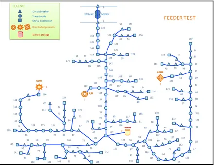
3.1. The test network

The test network used (8.4 kV), depicted in Fig. 1, consists of 162 MV nodes, 44 of which are secondary substations. It is connected to the HV network by a transformer 150/20 kV.

Fig. 1. Simplified scheme of the test network

Distributed energy resources in the test network are a photovoltaic (PHV) power plant at node 6, a gas turbine at node 7 and a wind power plant at node 8. The data of the distributed generators are reported in Table 1, where

Qmin and Qmaxare the lower and upper bounds to the reactive power production, An is the apparent power and

cosϕn is the power factor.

Table 1. Data of distributed generators.

generator Pmin _Pmax _Qmin _Qmax _A

n cosijn

[MW] [MW] [MVar] [MVar] [MVA] [-]

gas turbine 0.74 2.96 -1.11 2.22 3.7 0.8

wind power plant 0.34 1.36 -0.51 1.02 1.7 0.8

PHV power plant 0 1 - 0.484322 0.484322 1 1

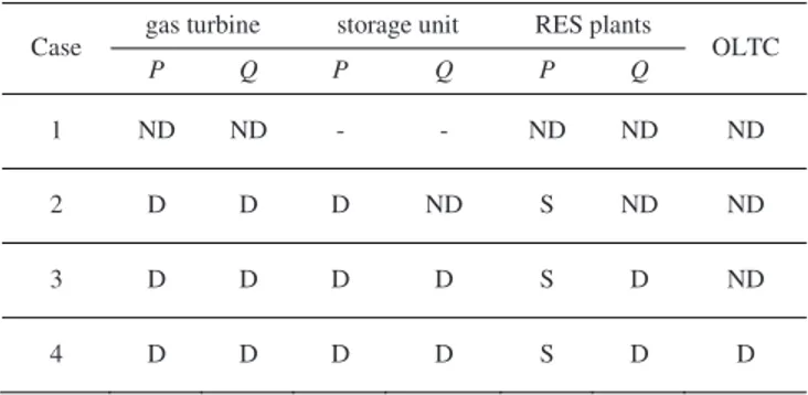
In the numerical experiments 4 cases of increasing complexity have been considered, corresponding to increasing flexibility in the network operation, as shown in Table 2. In Case 1 the DSO cannot control active (P) and reactive (Q) power production of the gas turbine and of RES power plants: gas turbine production is decided by the power producer; productions of Renewable Energy Source (RES) power plants depend on weather conditions (wind speed and solar radiation) and cannot be interrupted. As storage units are not available, active and reactive power balance can only be guaranteed by power exchanges with the HV network.

Table 2. Availability of regulation resources in the 4 cases considered

(ND: non dispatchable, D: dispatchable, S: interruptible)

Case gas turbine storage unit RES plants OLTC

P Q P Q P Q

1 ND ND - - ND ND ND

2 D D D ND S ND ND

3 D D D D S D ND

4 D D D D S D D

In cases 2, 3 and 4 a storage unit, whose characteristics are shown in Table 3, is assumed to be installed at node 9 and directly operated by the DSO. In Case 2 the DSO can dispatch active and reactive power of the gas turbine and active power of the storage unit. Moreover, the active power production of non programmable power plants can be interrupted. In Case 3 the DSO, together with the regulation resources available in Case 2, can also dispatch reactive power of the storage unit and of RES power plants, by means of inverters. Finally, Case 4 is the most flexible one, as On-Load Tap Changers (OLTC) HV/MV (150/20 kV) and MV/MV (20/8.4 kV) are added to the regulation resources available to the DSO in Case 3.

Table 3. Data of storage unit.

pmax emax einiz efin ηin _ηout _η

[MW] [MWh] [MWh] [MWh] [-] [-] [1/h]

2 2 0.2 0.2 0.9 1.1 0.995

The time horizon is one day, discretized in hours. In Step 1 the complete time horizon of 24 hours is considered; in Step 2 the small dimension of the test network allows to consider a time horizon of 12 hours (i.e. 1-12 and 13-24), which implies that Step 2 is performed only twice.

3.2. Starting point: active power balance based on forecasts of loads and of non programmable generation

In the numerical experiments forecasts of load and of non programmable generation are assumed to be available, as well as the scheduled generation of the gas turbine. In Fig. 2(a) and 2(b) hourly load forecasts are represented by yellow lines with dots, forecasts of production of RES power plants by red lines, the gas turbine scheduled generations by violet lines, the active power exchanges with the HV network by orange lines and the total active

power generated by blue lines, which coincide with the corresponding yellow lines, therefore showing that in both cases active power balance is attained in every hour. When storage is not available, the active power balance is satisfied by the active power exchanges with the HV network represented in Fig. 2(a). The optimal solution when storage is available is shown in Fig. 2(b): electricity is stored in hours 4 and 5, when its market price (to be paid for purchase from the HV grid) is less than the gas turbine production cost. The storage is fully discharged in hour 18, when the electricity market price reaches a peak, and is charged in hour 24, in order to guarantee the requested final value.

Fig. 2. Active power balance obtained by exchanges with HV grid (a) and by exchanges with HV grid and storage unit (b).

3.3. Computing an optimal solution for the AC network when realizations differ from forecasts

The realized values of loads and of non programmable generation are assumed to differ from forecasts, as shown in Fig. 3(a) and 3(b). In order to guarantee the balance of loads and generations, controllable resources have to be redispatched. We assumed the following order of priority, defined by the associated costs, for the use of the available regulation resources:

1) OLTC HV/MV and MV/MV;

2) reactive power of all generators and of the HV network; 3) active power of the storage unit;

4) active power of the gas turbine (constant value) and of the HV network (hourly market electricity price); 5) active power of RES power plants.

In the following we present and discuss the results obtained, in the four cases considered, by the two-step optimization procedure outlined in Section 2.

3.3.1. Step 1 of the optimization procedure (OPF_CC)

Given the realized values of loads and of RES generations, the hourly active power productions of programmable generators and the use of the storage unit, when available, are recomputed in Step 1, so as to guarantee active power balance, while minimizing the cost of the DSO control action. In case 1 (storage not available) the active power exchanges with the HV network, represented in Fig. 3(a), differ from the ones in Fig. 2(a), in order to compensate for the differences between forecasts and realizations. Fig. 3(b) shows that in cases 2, 3 and 4 (storage available) the differences between forecasts and realizations are mainly compensated by the storage unit, accordingly with the priority order introduced in Section 3.3.

Fig. 3. Step 1- Active power balance with realized values: (a) exchanges with HV grid only; (b) exchanges with HV grid and storage unit.

Fig. 4. Step 1- Hourly stored electricity: (a) based on forecasts; (b) based on realizations.

The hourly storage levels in the solution based on forecasts of load and of RES generation, represented in Fig. 4(a), can be graphically compared with the hourly storage levels in the solution based on their realizations, represented in Fig. 4(b).

3.3.2. Step 2 of the optimization procedure (OPF_AC)

In Fig. 5 it is shown how the active power balance, which takes into account active power losses, is attained in the four cases considered: the sum of hourly loads is represented by yellow lines with dots, the sum of power productions from RES by green lines, the gas turbine productions by violet lines, the exchanges with the HV network by orange lines, storage charge (negative values) and discharge (positive values) by blue rectangles and the total active power generated by blue lines, which coincide with the corresponding yellow lines, therefore showing that the active power balance constraints are satisfied in every hour in all cases.

Fig. 5. Step 2- Active power balance: (a) Case 1; (b) Case 2; (c) Case 3; (d) Case 4.

In Fig. 5(a) the solution for Case 1 is reported, in which the active power balance is guaranteed by the exchanges with the HV network. In Fig. 5(b) the optimal solution is depicted for Case 2, in which the storage unit is available, the gas turbine can be dispatched and RES generation can be interrupted. Comparison with Fig. 3(b) shows that active power balance in Step 2 is obtained by modifying the use of the storage unit computed in Step 1 and by decreasing the gas turbine production in hour 19. Analogously, the optimal solutions for Cases 3 and 4,

reported in Fig. 5(c) and Fig. 5(d), respectively, modify the use of the storage unit determined in Step 1 and decrease the gas turbine production in hour 12.

Fig. 6. Network losses of active power.

Network active power losses are represented in Fig. 6: it can be noticed that in cases 2, 3 and 4 the available regulation resources allow network losses (represented by the blue, green and violet lines, respectively) to be lower than in Case 1 (represented by the red line).

In Fig. 7 the storage levels at the end of every hour are represented for the solution computed in Step1 (red) and for the solutions computed in Step 2 in Case 2 (blue), in Case 3 (green) and in Case 4 (violet). In all cases the storage is mainly charged in hours 4 and 5, when the market electricity price is low, and discharged in hour 18, when the electricity price is high. In the solution computed in Step 1 the storage reaches its peak level in hour 5, to be subsequently discharged in hours 6-13; it is then charged in hours 15-17 and discharged in hour 18; in the last hours charge and discharge alternate and the minimum level requested in the last hour is satisfied. The solution computed in Step 2 satisfies the level constraint set by the solution computed in Step 1, namely 1.4 MWh at the end of hour 12, as well as the level constraints at the beginning of hour 1 (0.2 MWh), and at the end of hour 24 (0.2 MWh). Within these limits, the storage active power is redispatched, taking into account storage loss, which in Step 2 are more accurately represented than in Step 1, and network losses. In cases 3 and 4 it is also possible to dispatch the storage reactive power, which may affect the optimal values of the storage charge and discharge, in order to guarantee voltage constraints at all nodes.

Fig. 8. Voltage profile in hour 16.

In Fig. 8 voltages at every node in the four cases considered are shown for hour 16, the most critical one in terms of overvoltage (overpotential). The voltage maximum and minimum values have been set to ±10% of the network rated voltage (8.4 kV). In Case 3 (pink line) the range of node voltages is smaller than in Case 2 (dark brown line). Voltage drops are reduced as a consequence of a reduction of the reactive power generated by RES power plants, which cannot be dispatched in Case 2. In Case 4 tap-changers allow voltage of every node not to be near either its maximum or its minimum.

Fig. 9. Reactive power balance: (a) Case 1; (b) Case 2; (c) Case 3; (d) Case 4.

Fig. 9 shows how the reactive power balance is guaranteed every hour in the four cases considered. The following lines are shown in the graphs: sum of hourly loads (yellow); sum of reactive power produced by RES power plants in every hour (green); hourly reactive power production of the gas turbine (violet); exchanges with the HV network in every hour (orange); hourly contribution of the MV network (red); total reactive power generated in every hour (blue line coinciding with the yellow line, therefore showing balance between load and generation). Blue rectangles represent storage absorptions (negative values) and injections (positive values). In Fig. 9(a) the solution for Case 1 is reported, in which the reactive power balance is guaranteed by exchanges with the HV network only. In Fig. 9(b) the optimal solution is reported for Case 2, in which reactive power of both HV network and gas turbine can be dispatched. Comparison with Fig. 9(a) shows that a large reduction is requested to the gas turbine, in order to guarantee that voltage at every node is in the feasible range. In Fig. 9(c) the optimal solution is reported for Case 3, in which reactive power of HV network, gas turbine, RES power plants and storage can be dispatched. In order to avoid voltage range violations, large reductions are requested to both the gas turbine and the wind power plant. In some hours reactive power of photovoltaic plant and storage is also dispatched. In Case 4, as shown in Fig. 9(d), modifications of reactive power production requested to the gas turbine, the RES power plants and the storage, differ from the one requested in Case 3, due to the availability of the tap-changers.

Fig. 10: Variations of reactive power production requested in Step 2: (a) gas turbine; (b) wind power plant; (c) photovoltaic plant; (d) storage.

In order to satisfy voltage constraints at all nodes, variations of reactive power production may be requested to the controllable resources. Fig. 10 shows the requested variations with respect to the reactive power that corresponds, through the nominal power factor, to the active power production computed in Step 1. Fig. 10(a) shows the variations requested to the gas turbine: it can be noticed that in Case 2 (red), when gas turbine reactive power can only be dispatched, large reductions are requested than in Case 3 (green) and in Case 4 (violet), when the reactive power of RES power plants and of the storage unit can also be dispatched. Fig. 10(b) shows that in Case 4 (violet) smaller reductions are requested to the wind power plant than in Case 3 (green), with the exception of hours 4, 8, 9, 18, 19, 21, 22 and 24. Fig. 10(c) shows that in Case 3 (green) reductions are requested to the photovoltaic plant only in a few hours (i.e. 13, 17, 19, 22 and 24), while in Case 4 (violet) reductions are requested in all hours. For the storage unit Fig. 10(d) shows that in Case 3 (green) only two variations are requested, namely a reduction in hour 4 and an increase in hour 19, while in Case 4 (violet) a more intensive usage is determined, with variations requested in all hours, with the exception of hour 12.

Fig. 11. Active and reactive power flows and power factor at HV/MV node: (a) Case 1; (b) Case 2; (c) Case 3; (d) Case 4.

In Fig. 11 active power flows (blue line), reactive power flows (red line) and power factor at the HV/MV node (green line) are represented for the four cases considered. In all cases a relevant active power flow towards the HV network occurs in hours 8-11 and 16-21, when the gas turbine production is high. In Case 1, see Fig. 11(a), reactive power flows towards the HV network are also relevant in hours 8-11 and 16-21, as reactive power balance is obtained only by exchanges with the HV network; the power factor varies considerably along the time horizon and takes very small values in some hours, reaching the zero value when only reactive power flows. In Case 2, see Fig. 11(b), the reactive power flow towards the HV network has been reduced by redispatching the gas turbine reactive power and in some hours the HV network supplies a substantial amount of reactive power to the MV network; the power factor is near 1 (i.e. only active power is exchanged) in most hours, with the lowest value, 0.63, in hour 15. In Case 3, see Fig. 11(c), the reactive power flow towards the HV network occurs only in hour 4; the power factor is 1 in all hours but hour 4, where it takes value 0.63. In Case 4, see Fig. 11(d), very small quantities of reactive power flow towards the HV network in hours 14-21. In all hours, but hours 4, 6 and 7, the power factor is 1.

Fig. 12(a) shows the optimal positions in every hour of the tap-changer of the HV/MV transformer (150/20 kV). When generation of the gas turbine and of the RES power plants is high (hours 8-21), the optimal position of the tap changer is above the central one, which allows to reduce the network voltage. When load and generation are low (hours 1, 2, 3, 5, 22, 23 and 24), the optimal position of the tap changer is below the central one, so as to increase the network voltage and therefore reduce current transits and active power losses. The optimal positions of the tap-changer of the MV/MV transformer (20/8.4 kV) in every hour are shown in Fig. 12(b). In hours with

high generation of the gas turbine and of the RES power plants the network voltage is reduced by setting the tap changer above the central position.

Fig. 12. Case 4: optimal positions of tap-changers: (a) HV/MV; (b) MV/MV.

4. Conclusions and current work

A two-step procedure has been proposed for determining the optimal control actions to be taken by the DSO when realized loads and RES generations differ from forecasts. The procedure is based on decoupling integrality and nonlinearity, in order to avoid high computational costs in real problems when the MV network dimension is large. Results of some numerical tests are reported, concerning four alternative hypotheses on the regulation

resources available to the DSO. In Case 1 active power losses are higher than in cases 2, 3 and 4; in some hours voltage constraints at some nodes are violated, as well as current constraints in some lines, i.e. exchanges with the HV network cannot guarantee security and power quality in some hours; finally, reactive power absorption by the HV network is required in many hours, in order to balance generation and load. In Case 2 the reactive power absorption by the HV network is greatly reduced, as the DSO can request a reduction of the gas turbine reactive power production; in cases 3 and 4, in which reactive power production of all generators can be controlled, the reactive power load is satisfied by the MV network distributed generators. In Case 3 the possibility of reducing reactive power production of RES power plants allows a smaller gap, with respect to Case 2, between the highest and the lowest node voltages. In Case 4 voltages at all network nodes in the optimal solution are far away from their lower and upper limits, which is however obtained by varying the steps of tap-changers at every time unit. The regulation resources in cases 3 and 4, therefore, yield the best solutions for the test network under consideration, with case 4 possibly affected by tap changer deterioration.

Fig. 13. Voltages at nodes and currents in lines for Case 1.

In Fig. 13 a display diagram is provided which shows voltages at nodes and currents in lines for Case 1: for green nodes voltages are within the imposed limits, while for violet nodes overvoltage occurs. For green and yellow lines currents are within the imposed limits, while for red lines the limit is approached.

The display diagram in Fig. 14 shows voltages at nodes and currents in lines for the optimal solutions of Case 3. Overvoltage is solved (all nodes are green) and in some lines current transits are reduced, as a consequence of the reduction of reactive power produced by the distributed generators.

Fig. 14. Voltages at nodes and currents in lines for the optimal solution of Case 3.

The proposed procedure can be used a simulation tool for the DSO to optimize the configuration of MV network, e.g. determine effective positions of storage units. It can also be used by regulators as a simulation tool to analyze the impact of costs associated to the usage of controllable resources. New tests of the procedure are planned in the near future on a real-life large scale prototype network in Italy.

References

Garzillo, A., Gelmini, A., Moneta, D., Siface, D., Vespucci, M. T., & Innorta, M. (2012). Sviluppo di OPF in AC multi periodo per la gestione centralizzata di elementi di accumulo. RSE report 12000908, www.rse-web.it.

Garzillo, A., Innorta, M., & Ricci, M. (1998). The problem of the active and reactive optimum power dispatching solved by utilising a primal-dual interior point method. International Journal of Electrical Power & Energy Systems, 20(6), 427 – 434.

Mehrotra, S. (1992). On the implementation of a primal dual interior point method. SIAM Journal on Optimization 2(4),575 – 601.

Moneta, D., Carlini, C., & Belotti, M. (2011). Specifiche dell’algoritmo per il controllo di tensione ai nodi e di corrente nelle linee di una rete attiva. RSE report 11000886, www.rse-web.it.