2020-03-26T16:09:35Z
Acceptance in OA@INAF
þÿAbundance patterns in early-type galaxies: is there a "knee" in the [Fe/H] vs. [±/Fe]
relation?
Title
Walcher, C. J.; Coelho, P. R. T.; GALLAZZI, Anna Rita; Bruzual, G.; Charlot, S.; et
al.
Authors
10.1051/0004-6361/201525924
DOI
http://hdl.handle.net/20.500.12386/23605
Handle
ASTRONOMY & ASTROPHYSICS
Journal
582
Number
10.1051/0004-6361/201525924
c
ESO 2015
Astrophysics
&
Abundance patterns in early-type galaxies: is there a “knee”
in the [Fe/H] vs. [
α
/Fe] relation?
C. J. Walcher
1, P. R. T. Coelho
2, A. Gallazzi
3,4, G. Bruzual
5, S. Charlot
6, and C. Chiappini
11 Leibniz-Institut für Astrophysik Potsdam (AIP), An der Sternwarte 16, 14482 Potsdam, Germany
2 Instituto de Astronomia, Geofísica e Ci˜encias Atmosféricas, Universidade de São Paulo, Rua do Matão 1226, 05508-090 São Paulo,
Brasil
3 INAF-Osservatorio Astrofisico di Arcetri, Largo Enrico Fermi 5, 50125 Firenze, Italy
4 Dark Cosmology Center, University of Copenhagen, Niels Bohr Institute, Juliane Maries Vej 30, 2100 Copenhagen, Denmark 5 Centro de Radioastronomía y Astrofísica (CRyA), Morelia, 58089 Michoacan, Mexico
6 UPMC-CNRS, UMR7095, Institut d’Astrophysique de Paris, 75014 Paris, France
Received 18 February 2015/ Accepted 18 August 2015
ABSTRACT
Early-type galaxies (ETGs) are known to be enhanced in α elements, in accordance with their old ages and short formation timescales. In this contribution we aim to resolve the enrichment histories of ETGs. This means we study the abundance of Fe ([Fe/H]) and the α-element groups ([α/Fe]) separately for stars older than 9.5 Gyr ([Fe/H]o, [α/Fe]o) and for stars between 1.5 and 9.5 Gyr ([Fe/H]i,
[α/Fe]i). Through extensive simulation we show that we can indeed recover the enrichment history per galaxy. We then analyze a
spectroscopic sample of 2286 early-type galaxies from the SDSS selected to be ETGs. We separate out those galaxies for which the abundance of iron in stars grows throughout the lifetime of the galaxy, i.e. in which [Fe/H]o< [Fe/H]i. We call those consistent with
self-enrichment, while the others must have experienced some mergers or significant gas accretion. We confirm earlier work where the [Fe/H] and [α/Fe] parameters are correlated with the mass and velocity dispersion of ETGs. We emphasize that the strongest relation is between [α/Fe] and age. This relation falls into two regimes, one with a steep slope for old galaxies and one with a shallow slope for younger ETGs. The vast majority of ETGs in our sample do not show the “knee” in the plot of [Fe/H] vs. [α/Fe] commonly observed in local group galaxies. This implies that for the vast majority of ETGs, the stars younger than 9.5 Gyr are likely to have been accreted or formed from accreted gas. The properties of the intermediate-age stars in accretion-dominated ETGs indicate that mass growth through late (minor) mergers in ETGs is dominated by galaxies with low [Fe/H] and low [α/Fe]. The method of reconstructing the stellar enrichment histories of ETGs introduced in this paper promises to constrain the star formation and mass assembly histories of large samples of galaxies in a unique way.
Key words.galaxies: abundances – galaxies: stellar content – galaxies: elliptical and lenticular, cD
1. Introduction
The stars in massive early-type galaxies (ETGs) have had to form early in the history of the universe for two reasons: 1) Very few of these galaxies have (significant) young stellar populations (e.g., Yi et al. 2005;Trager & Somerville 2009;Thomas et al. 2010) and 2) the ratio of α elements (O, Mg, etc.) to Fe in the atmospheres of these stars is higher than solar (e.g., Peterson 1976; Worthey et al. 1992; Milone et al. 2000), indicating a short timescale for the enrichment of the ISM out of which they formed. The ratio [α/Fe] is a powerful estimator of the duration of star formation (Tinsley 1979; Matteucci & Greggio 1986). Study of the mass dependence of the ages and enhancement ra-tios of ETGs has led to the classical picture in which the star formation timescales are shorter with increasing galaxy mass (Thomas et al. 2005).
Direct studies of massive galaxies at high redshift support this picture in which at least some ETGs must have “formed the bulk of their mass only a few million years after the big bang” (Nayyeri et al. 2014). On the other hand there is evidence that massive ETGs cannot be described by a stellar population with a single age and abundance pattern (recently, e.g.,Lonoce et al. 2014). Indeed,Arimoto & Yoshii(1986) emphasize that this is true in terms not only of an age spread, but also of an abundance
spread: “The present analysis shows that such metal-poor stars in the RGB evolution have a strong influence on the integrated colors of the galaxy”.
Recent observational and theoretical work has focused on the question of when and how the late mass growth of early-type galaxies takes place. Two opposite possibilities for such mass growth exist: 1) in situ star formation from gas that was ac-creted in the initial phase of the galaxies formation and 2) mass growth from later major or minor dry merging. A third possi-bility with less clear observational signatures is 3) stellar mass growth through star formation from gas that was either accreted during a merger (wet mergers) or in a cold mode from the cosmic web.
Different observational approaches to these questions ex-ist. An important piece of the puzzle is the observation that the progenitors of ETGs at redshifts above z ∼ 1 are com-pact, dense objects (Trujillo et al. 2006; van Dokkum et al. 2008; van der Wel et al. 2008). Naab et al. (2009), Hopkins et al. (2009), and van Dokkum et al. (2010a) show that the cores of today’s ellipticals are consistent with being the dense galaxies observed at high redshift, althoughvan der Wel et al.
(2011) make the point that the majority of these distant, dense galaxies should be thought of as disk-like, introducing some tension with the mostly dispersion-dominated cores of today’s
early-type galaxies. Overall, the data have led to the notion that (minor) merging over a Hubble time will simultaneously con-tribute to the mass growth of these objects and to their size growth (Clemens et al. 2009; Naab et al. 2009; van Dokkum et al. 2010a;Oser et al. 2012;Greene et al. 2012,2013).
Simulations predict that stellar accretion is most important at large radii (Lackner et al. 2012;Navarro-González et al. 2013;
Hirschmann et al. 2015). In contrast to earlier notions, simula-tions even show that no major merger at all is needed to form massive ellipticals (Bournaud et al. 2007). On the other hand, direct measurement of major merging is available in the litera-ture (e.g.,Bell et al. 2006;de Ravel et al. 2009;Robaina et al. 2010; Robotham et al. 2014). These studies find that the typi-cal L* galaxy will have undergone one major merger after red-shift one (Keenan et al. 2014) and that the higher the mass of a galaxy, the more it grows through major merging. The evo-lution in the mass function can be combined with the expected growth due to star formation to yield a direct measure of the mass growth due to mergers in ETGs (Walcher et al. 2008;
Ownsworth et al. 2014). This leads to estimates of roughly half of the present-day total stellar mass of ETGs being formed in other galaxies prior to their incorporation into the ETG over cos-mic time. However, mergers also contribute gas. For example
Kormendy et al.(2009) discuss how structural properties can be used to distinguish between dry mergers that would contribute only stars and wet mergers that would in turn contribute gas, thus leading to late star formation and rebuilding of cusps.
The present paper is dedicated to measuring the relative im-portance of the mass-growth processes from their chemical sig-nature. In particular, other observational approaches cannot hope to distinguish between in situ formation of stars from gas left over from any putative “initial accretion”, on the one hand, and gas subsequently accreted either in a cold mode or through mi-nor mergers, on the other. This distinction is much easier to study from chemical signatures as shown below.
In this contribution we define the stellar enrichment histo-ries (SEH) as the four-dimensional space occupied by the stellar populations in each galaxy and spanned by the parameters age (i.e., time elapsed since formation of those populations), [Fe/H], [α/Fe] and the mass (or luminosity) contribution of these stars. It needs to be kept in mind that we can only address the stel-lar population within one spatial resolution element (one fiber in our case, the case of SDSS). Because of measurement uncer-tainties we very strongly bin this space into just two age bins: the old age bin contains all stars older than 9.5 Gyr, the interme-diate age bin contains all stars between 1.5 and 9.5 Gyr of age. Within each age bin and for each galaxy we can compute the luminosity-averaged [Fe/H] and [α/Fe] as well as the fractional contribution of the old and intermediate populations to the total luminosity of each galaxy. This principle is illustrated in the up-per panel of Fig. 1. For the remainder of this paper we denote the mean [α/Fe] and [Fe/H] of the old stars with the subscript “o” (i.e. we write [Fe/H]oand [α/Fe]o), whereas we denote the mean [α/Fe] and [Fe/H] of the intermediate age stars with the subscript “i” (i.e. we write [Fe/H]i and [α/Fe]i). The “star for-mation history” (SFH) would simply be the marginalization of the SEH onto the 2-dimensional space of age and luminosity contribution.
The choice of 9.5 Gyr for separating old and intermediate stellar populations in ETGs is of course to some level arbitrary. It can, however, be justified on several grounds as providing the widest age bin for old stars that still makes sense physi-cally. On the one hand simulations such as those ofNaab et al.
(2009) show the typical mass assembly histories of ETGs in
Fig. 1.Schematic representation of the new parameters introduced in
this paper, namely [α/Fe]o and [Fe/H]o. These represent the average
[α/Fe] and [Fe/H] of stars older than 9.5 Gyr on a per galaxy basis. The upper panel shows a schematic star formation history, which sepa-rates into these two stellar populations. The lower panels depicts on the standard [α/Fe] vs. [Fe/H] diagram familiar for the Milky Way what is expected for the old and intermediate age stars respectively.
a hierarchical universe. For many of these galaxies there is a change of regime at around 10 Gyr ago, where the mass build-up changes from being dominated by in-situ star formation to accretion of other, smaller galaxies and clumps. Thus this is an age where we expect to maximize the signal from any differ-ence between old and intermediate age population. On the other hand, those alpha-enhanced populations that we can study in de-tail in the Milky Way are all older than 11 Gyr. This is true for the thick disk (Fuhrmann 2011) and for the bulge (Bensby et al. 2013). As shown later in the present paper (Fig. 12, lower right panel) and in a paper in preparation (Walcher et al., in prep.), this effect is seen in the luminosity-weighted average properties at a lookback time of around 9.5 Gyr as well in the sense that the rate of change of [α/Fe] with time shows a significant change of slope. These 2 or 3 Gyr after the onset of star formation are thus different in the chemical signatures, which helps for the techni-cal as well as scientific arguments of the present paper. Finally, the cosmic star formation density peaks at a lookback time of 10 Gyr, as shown in the recent review byMadau & Dickinson
(2014, their Fig. 9). Specifically for ETGs, this is also the time when quiescent galaxies started appearing in large number (see e.g.,Arnouts et al. 2007, their Fig. 13).
The lower panel of Fig.1 illustrates basic expectations for the locus the old and intermediate stellar population would occupy in the projection onto the [α/Fe] vs. [Fe/H] plane. As is well known the “knee” in this diagram carries information about the star formation efficiency in the galaxy, where higher star
formation efficiency leads to higher overall metallicity before the onset of SNIa enrichment, and thus to a knee that is located at higher [Fe/H] values. The low-[Fe/H] plateau in [α/Fe] can be modulated by the slope of the upper end of the stellar initial mass function, but the data we discuss here do not allow any inference concerning this, thus we neglect this question for the remainder of the paper.
The existence of the knee in the lower panel of Fig.1 for the Milky Way stars is tied to some causal connection at each time step during the star formation history between the existing stars and the next generation of stars. Although some accretion is needed, if only to solve the g-dwarf question, we generally call this a scenario that is consistent with self-enrichment (SLF). The SLF scenario would predict in our specific case of coarsely resolved enrichment histories for ETGs that the [Fe/H] of the intermediate-age population would always be higher than for the old population and the [α/Fe] of the intermediate-age pop-ulation would always be lower than that of the old poppop-ulation. On the other hand, as mentioned above we know that mergers contribute a significant percentage of the stars in massive ETGs. The merging stars bear no connection to the pre-existing stars in the ETG and thus could have any [Fe/H] and [α/Fe] properties. The shorthand for this scenario throughout this paper is ACC for accretion.
The mass-metallicity relation (Tremonti et al. 2004;Gallazzi et al. 2005) leads to the expectation that minor, i.e. low mass mergers would contribute stars with sub-solar [Fe/H]. The [α/Fe] of these stars is less certain. However, Sansom & Northeast(2008) show that the high [α/Fe] abundances seen in
massive quiescent galaxies do not continue to the lower lumi-nosity quiescent galaxies, as those have generally lower [α/Fe]. Also, lower mass galaxies tend to have prolonged star formation histories, again leading to an expectation of lower [α/Fe] in gen-eral. We caution that we currently do not know what the [α/Fe] of intermediate-redshift minor mergers could be. Nevertheless, we are led to an expectation that the intermediate-age stars in ETGs would on average have solar [α/Fe] and [Fe/H] either slightly above or even significantly below the solar value (the blue el-lipse in Fig.1). Indeed,Coelho et al.(2009) found that for the galaxy M32 the metal-poor component of their stellar popula-tion fit corresponds to a younger populapopula-tion than the metal-rich one.
Although simple, this picture can be used to provide a frame-work for interpreting the results in this paper. Complications arise, however, that need to be acknowledged. For example,
Pipino et al. (2009) show that semi-analytic models cannot re-produce the [α/Fe]-mass relations yet, owing to inadequate treat-ment of late mergers, thus clearly implying that we do not have sufficient theoretical understanding of low-mass galaxy evolu-tion in simulaevolu-tions. More generally, Hirschmann et al. (2013) conclud that, while it is clear that accretion, minor merging, major merging, star formation efficiency, and winds must all work together to form those galaxies we see today, their ex-act interplay is still not sufficiently understood. Simulations thus do not produce a satisfying population of galaxies over-all. Observationally, and in the direct context of this contribu-tion, this is illustrated by the recent work ofRenzini & Andreon
(2014), who concluded from data on the enrichment of the intra-cluster medium “that even the most massive galaxies must have lost a major fraction of the metals they have produced”.
An uncertainty that much more directly affects our distinc-tion in SLF and ACC ETGs has been spelled out in the works of
Arimoto & Yoshii(1986) andVazdekis et al.(1996). Indeed, it turns out that metallicity may not monotonously increase with
age for the most massive ETGs even in absence of accretion events. After a peak in metallicity at a certain age, this metal-licity starts declining again because of the late mass loss by the abundant low-metallicity stars still present in the galaxy. Comparison with Fig. 11 ofVazdekis et al.(1996) reveals that the peak in metallicity may be reached very rapidly (within 2 or 3 Gyr after formation of the galaxy). However, the decline in metallicity remains subtle and is of order 0.2 dex in [Z] until redshift zero. We come back to this value in Sect.6.3.
The present contribution introduces extensions to the method of spectral fitting. We therefore present our algorithm in detail in Sect. 3 and then spend significant space on understanding any possible method-intrinsic effects, such as degeneracies, in Sect.4. Finally we also verify in detail that the method is ap-plicable to the data at hand in Sect.5. Readers wishing to read about the scientific results first can jump directly to Sect.6. 2. Sample
For this paper we are interested in a significant sample of early-type galaxies (ETGs) with high signal-to-noise ratio (S/N) spec-tra. With ETG we mean a “spectral ETG”, i.e. essentially a galaxy with a spectrum dominated by old stars. Such a sample is easily selected from the MPA/JHU catalogs1 for SDSS DR7 (Abazajian et al. 2009), containing general information about the galaxy’s spectrum (S/N, stellar velocity dispersion), emission lines and absorption indices, as well as photometric information. ETGs in the SDSS have been studied in many contributions to the literature (e.g.,Bernardi et al. 2003;Zhu et al. 2010). The specific reason to revisit these spectra is that they provide a large sample of readily available high quality spectra with which to test the power of the new models and the new methodology we apply here. In particular we adopt the following criteria to select our sample:
– S/N larger than 40;
– r-band concentration index larger or equal to 2.8;
– unclassifiable, i.e. with S/N < 3 in all of the BPT diagram emission lines, thus excluding AGN;
– velocity dispersion between 40 and 375 km s−1;
– eliminate duplicate observations, keeping the one with higher S/N.
We further estimate stellar masses from absorption indices fol-lowing the exact same method as Gallazzi et al. (2005). The sample is thus further restricted to those galaxies for which a spectroscopic stellar mass could be obtained (i.e. for which the set of five absorption features, r − i fiber color and z-band model magnitude are available). We use the 16, 50, 84 percentiles of the probability distribution function for the lower 1σ errorbar, the actual value and the upper 1σ error bar, respectively. These masses are normalized to the z-band modelmag and a Chabrier IMF.
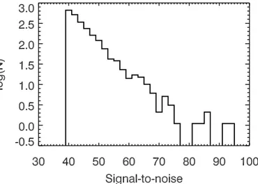
These criteria give us a sample of 2286 pure early-type galaxies. This sample has been S/N selected and it would thus be a daunting task to follow through all selection criteria to infer how representative the sample is for all early-type galaxies. We thus refrain from such an exercise. The S/N distribution of our sample is shown in Fig.2.
3. Stellar population models and fitting procedure Stellar population models exploring the effects of varying ele-ment abundance ratios on specific line indices have been driving
Fig. 2.S/N distribution of our sample galaxies.
our understanding of ETG formation and evolution (e.g., Lee et al. 2009). In particular, studying the dependancies of single elements (e.g.,Smith et al. 2009;Worthey et al. 2014) is inter-esting in its own right, but is currently not possible for the goals of this paper for two reasons: 1) We want to study SEHs in a resolved way and it would be difficult to control physical degen-eracies. 2) We need spectral models with a restricted set of free parameters to keep our algorithms mathematically under con-trol. Taking e.g. the recent contribution byWorthey et al.(2014) as a comparison and referring back to Fig. 1we can highlight one important point of our paper. These authors consider abun-dance distribution functions (ADFs) within each ETG to address the similar questions to the present contribution, namely how abundance ratios are spread within ETGs. However, due to the nature of the fitting algorithmWorthey et al.(2014) have to pa-rameterize these ADFs, thus leading to a prior assumption on the SEHs possible in the galaxies they analyze. Because knowl-edge of the real SEHs of ETGs is so scarce we do not believe that putting such a prior is warranted yet. In support of our ap-proach we also highlight that the use of [α/Fe] as a single pa-rameter involving a set of elements is also justified by the find-ings of Johansson et al.(2012), who find that the correlations of [O/Fe], [Mg/Fe], [C/Fe] with velocity dispersion are identical for ETGs. In general, models capable of predicting the effects of α-elements on the full optical spectrum of stellar populations are starting to become less rare, seeCoelho et al.(2007),Koleva et al. (2008b), Walcher et al. (2009), Percival et al. (2009),
Vazdekis et al.(2011),Conroy & van Dokkum(2012),Prugniel & Koleva(2012),Vazdekis et al.(2015).
We use an updated version of the differential stellar popula-tion models presented inWalcher et al. (2009, hereafter W09) and we refer to that paper for a full description. In brief, to compute the models we combine the simple stellar population (SSP) spectra from fully theoretical stellar population models byCoelho et al.(2007) (based on isochrones fromWeiss et al. 2007) with semi-empirical models byVazdekis et al.(2010) and
Falcón-Barroso et al.(2011). Of theVazdekis et al.(2010) mod-els we only use those with solar metallicity and abundance ra-tios. The model spectra for non-solar [Fe/H] and [α/Fe] values are then obtained using the C07 models of the same age as a prediction for the effects of varying [Fe/H] and [α/Fe]. We show in W09 that these models yield reliable values for the ages, the [Fe/H] and the [α/Fe] values of Milky Way globular clusters within the range covered by our models.
During the course of the project we realized that the parame-ter coverage of theCoelho et al.(2007) models (age: 3−12 Gyr, [Fe/H]: −0.5, −0.25, 0.0, 0.2 and [α/Fe]: 0.0, 0.4) lead to “edge effects”, in the sense that when fitting a stellar population older than 12 Gyr and with solar abundance ratios, age-metallicity de-generacy will drive the best-fitting model to have super-solar [Fe/H] and [α/Fe]. We have therefore decided to extrapolate the grid of theoretical models to an age range of 2−13 Gyr, [Fe/H] values of −0.5, −0.25, 0.0, 0.2 and [α/Fe] values of −0.2, 0.0, 0.2, 0.4. The theoretical spectra are interpolated linearly in a multi-dimensional space with the axes: pixel, log(Flux), age, [Fe/H] and [α/Fe] before being applied to the semi-empirical models.
Metallicity is defined as a combination of [Fe/H] and [α/Fe], explicitly for our models [Z] = [Fe/H] + 0.75 * [α/Fe] (see
Coelho et al. 2007).
Although we select galaxies for our analysis that have all signs of lacking young stellar populations, we cannot rule out any contribution. In the literature, rejuvenation of ETGs is still a controversial subject with findings related to sample definition, analysis methods and uncertainties related to late, hot phases of stellar evolution ([Fe/H] Yi et al. 2005;Sánchez-Blázquez et al. 2009;Ocvirk 2010;Thomas et al. 2010). We therefore extend our template set by five templates fromVazdekis et al.(2010) with younger ages (1, 0.63, 0.32, 0.1, 0.06 Gyr). These do not have varying [α/Fe] ratios. We include these templates into the fitting in all cases and use them to verify that indeed contribu-tions by younger stellar populacontribu-tions are negligible in the data we analyze.
Full spectrum fitting has survived a number of stringent tests ([Fe/H] Cid Fernandes et al. 2005; Koleva et al. 2008a) and is becoming increasingly popular as a method to derive stellar population properties of galaxies ([Fe/H] Heavens et al. 2000;
Cappellari & Emsellem 2004;Cid Fernandes et al. 2013, to cite but a few). For analysis of the spectra using full spectrum fit-ting we use the software paradise. The underlying algorithm is fully described in AppendixAand the same software was used in our previous papers (Walcher et al. 2006,2009). In one sen-tence, paradise fits model template spectra to observed spectra taking into account the uncertainties on each spectral pixel, solv-ing for the kinematics of the stellar population and allowsolv-ing very flexible masking of wavelength regions due to quality concerns.
4. Analysis of mock galaxy spectra
The goal of this paper is to shed new light on the SEHs of early-type galaxies to understand their formation history. Before we can do so, we must verify that our method is in principle capa-ble of providing us with SEHs. In the present section we describe the creation of mock galaxy spectra and their analysis. As we use the same models for the mock spectra as we then use to analyze these, we can only test the accuracy and intrinsic degeneracies of our method under the assumption that the model is a perfect rep-resentation of the data. We performed an independent test of the accuracy of our models as compared to globular cluster spec-tra inWalcher et al.(2009). In the remainder of the paper we report what we find when fitting the wavelength range 4828 to 5364A. This wavelength range has been shown in W09 to most accurately recover age, [Fe/H] and [alpha/Fe] for bulge globular clusters.
The main conclusion of this section is that we can recover the luminosity-weighted average properties of ETGs and the el-ement abundance patterns of their old stars with good accuracy
and precision. Recovering the properties of intermediate-age stars is a more challenging task.
4.1. Mock galaxy spectra
As motivated in the introduction, we analyze the SEHs of our galaxies in three bins of age τ, namely τ ≤ 1.5 Gyr (called young age bin from now on), 1.5 Gyr < τ ≤ 9.5 Gyr (called intermediate-age bin, subscript i), τ > 9.5 Gyr (called old age bin, subscript o). We do not attempt a better time resolution for the reasons given below and because experience with full spectrum fitting shows that three bins in age are a reasonable assumption for the best age resolution one can hope for in the star formation history (compare e.g.Cid Fernandes et al. 2005;
Tojeiro et al. 2007). We therefore construct our mock galaxies by separating our SSPs in the three age bins above and assuming a constant SFR within each of these bins. We then go on to ne-glect the youngest age bin, as any young stars (or hot stars, to be more precise), if present, represent a very small fraction of the light for the large majority of early-type galaxies (90%Thomas et al. 2010).
We then compute a grid of mock galaxies over the follow-ing parameter ranges: [Fe/H]i and [Fe/H]o vary between −0.5 and 0.2, [α/Fe]iand [α/Fe]o very between −0.2 and 0.4 and the mass contribution of the intermediate stars to the total stellar mass may vary between 0 and 100%. We note that we thus do notassume an exponentially falling star formation history at any point. On the other hand, for this exercise we divide the SFH of our mock galaxies in two age bins with constant star for-mation rate. Our grid of models is probably more varied than real early-type galaxies, in particular concerning the contribu-tion of intermediate-age stars, and thus any conclusions we de-rive from here is applicable to a more restricted set of SFHs as well. All model spectra are convolved with a velocity dispersion of 150 km s−1. We verified that our results do not depend on velocity dispersion, as long as this parameter is correctly deter-mined. One of the advantages of full spectrum fitting is that the velocity dispersion is determined simultaneously with the stel-lar population analysis, thus avoiding some of the potential pit-falls with the more classical Lick index method. Guided by the S/N distribution of our sample (see Fig.2), we perturb the spec-tra assuming Gaussian uncertainties to the lowest S/N ratio of the sample, i.e. 40.
4.2. Recovery of light-weighted mean quantities
We now use paradise to recover the following quantities: – V-band light-weighted mean parameters age, [Fe/H], [α/Fe],
Z
– V-band light-weighted mean parameters for old component ageo, [Fe/H]o, [α/Fe]o, Zo
– V-band light-weighted mean parameters for intermediate component agei, [Fe/H]i, [α/Fe]i, Zi
The mathematical equation defining these values as imple-mented by paradise is hXi= PN i=0aiLViXi PN i=0aiLVi , (1)
where ai are the weights for N templates with properties Xias well as V-band luminosities LV
i. This equation can also be used to define the same quantities over a restricted range of SSPs that
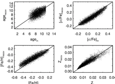
Fig. 3. Simulations of parameter recovery for a randomized coverage
of parameter space and a total of 3000 mock galaxies.
are part of the SEH (e.g. those representing only old or only intermediate-age stars) by suitably restricting the indices over which the sum is computed.
Our results for the overall light-weighted quantities, i.e. when the index i in Eq. (1) runs over all templates, are sum-marized in Fig.3.
Koleva et al. (2008b) andSánchez-Blázquez et al. (2011) study the influence of a metallicity – velocity dispersion degen-eracy, implying that when both parameters are fitted ously, the velocity dispersion may be underestimated simultane-ously with the metallicity or [Fe/H]. We find the opposite effect in our simulations, i.e. for lower values of [Fe/H] velocity dis-persion will be over-estimated slightly (for our fiducial value of 150 km s−1the overestimate is of order 10 km s−1 at [Fe/H] = −0.3). We observe no dependence on [α/Fe].Sánchez-Blázquez et al.(2011) emphasize that the effect is larger for young stellar
populations, while our study here focusses on old stellar pop-ulations. Also, we are not interested in the velocity dispersions here, but in the parameters age, [Fe/H] and [α/Fe]. Any influence of this metallicity – velocity dispersion degeneracy would show up in our study as a bias in [Fe/H] recovery. Indeed, this may be the reason for the slight deviation from a perfect recovery at low metallicities observed in our simulations.
We also explicitly test the influence of either normaliz-ing (rectifynormaliz-ing) or not normaliznormaliz-ing the spectra with a pseudo-continuum based on a running mean. We find that the fit with non-normalized continuum is formally slightly better, as ex-pected due to the higher information content. We caution, how-ever, that this is true for the ideal case we can test here, i.e. where the model and the “data” ideally match each other. Even a slight problem with flux calibration would potentially bias our results, we thus always normalize spectra from real data below.
The age-metallicity degeneracy is a long-standing problem in the study of old stellar populations. In the lower left panel in Fig.4one can read of that the effect is of order 0.1 dex in [Fe/H] per 2 Gyr. Here we refrain from performing a formal fit to the simulated data. This would only pretend to provide more precise information as it is entirely unclear how the mock galaxy sample would relate to either the sample under study here or the real full galaxy population. Comparison withThomas et al.
(2005, their Fig. 3),Cid Fernandes et al.(2005, their Fig. 6), and
Sánchez-Blázquez et al.(2011, their Fig. 7) shows that the trends are qualitatively the same, confirming once more that this effect
Fig. 4.Degeneracies in the overall mean light-weighted values as dif-ference plots. Each∆ is defined as the recovered minus the true value. The dominating degeneracy occurs between age and [Fe/H], while age and [α/Fe] show only weak degeneracy.
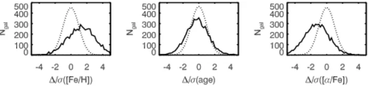
Fig. 5. Verification of the uncertainties derived by the fitting routine
through bootstrap. Each∆ is defined as the recovered minus the true value, but this time divided by the size of the error bar (denoted σ) as output by the fitting routine. For perfectly Gaussian errors, the distribu-tion should coincide with a Gaussian of width one and normalized to the same total area (dotted line).
is physical and does not depend on the fitting algorithm being ap-plied. In particular it is surprisingly independent of whether the fitted stellar population is a SSP or the fitting algorithm allows for a more complex star formation history. To be more precise, the degeneracy is between [Fe/H] and age. There are degenera-cies between age and [α/Fe], and between [Fe/H] and [α/Fe], but these are much less pronounced.
A new problem in the analysis of integrated spectra from ETGs are the many lines of evidence for a variation in the ini-tial mass function of galaxies (van Dokkum & Conroy 2010b;
Cappellari et al. 2012).Ferré-Mateu et al. (2014) explore how such variations would affect the analysis of the SFHs of ETGs and find that complete neglect of IMF variations would po-tentially significantly affect the results in particular in terms of the relative contribution of old and intermediate-age stars. Incorporating this caveat into our analysis is at present beyond the scope of this contribution.
As described in Appendix A, paradise performs a
bootstrap estimate of errors on the recovered stellar popula-tion parameters. Figure5verifies that these errorbars are appro-priate. Indeed, for correctly estimated Gaussian errorbars, the histogram of the quantity ∆(X)/σX should be a Gaussian with width 1, where∆(X) = Xmeasured− Xtrue. This is almost exactly the case for age and the widths of the distributions in [Fe/H] and [α/Fe]. There are systematic offsets for [Fe/H] and [α/Fe]. Given the average error bars from the simulations these translate to a systematic overestimation of [Fe/H] by 0.07 dex and an under-estimation of [α/Fe] by 0.03 dex. Figure3shows that the largest offset of ∼0.1 dex occurs at low values of [Fe/H].
Fig. 6.Simulations of parameter recovery when splitting the star
forma-tion and enrichment history at a fiducial age of 9.5 Gyr. The dashed line in the lower right panel is a formal fit to the points in the data with a slope of ∼0.3.
4.3. Can we resolve the enrichment histories?
The term SEH implies the wish to represent the relation between age and abundance for each galaxy. To our knowledge this has not been done in the literature. Whilede La Rosa et al.(2011) have applied the spectral fitting technique to the SFH, they have not actually resolved the SEH, preferring to quote a single value for the enhancement in α-elements. We thus here investigate in detail, whether our method is able to produce this kind of infor-mation reliably. We thus repeat the same plots of input vs. recov-ered quantities as in Sect.4.2for the properties [Fe/H]o, [α/Fe]o, [Fe/H]i, [α/Fe]i. The result is shown in Fig. 6. To economize some space, we do not plot ages and metallicities for the old and intermediate distinction. The reason is that the ages are fixed already by the way we separate the star formation history into bins and its recovered distribution therefore carries no real mean-ing (although it can vary slightly within the width of that bin). Metallicity on the other hand is only a trivial combination of [Fe/H] and [α/Fe].
Figure6looks encouraging concerning the old stars in that clear relations scattering around the one-to-one line exist, with an RMS width of about 0.1 dex. While it may not seem intu-itive at first sight that the properties of the older stellar popu-lation, which contributes on average less to the total light than the younger or intermediate-age population, would be well-determined from a fit to the integrated spectrum, this is actu-ally in line with the findings ofSerra & Trager(2007). These authors found that the SSP-equivalent chemical composition de-pends mainly on the chemical composition of the older of two constituting stellar populations. It is also in line with theoreti-cal expectations that the effects of [α/Fe] (in particular Mg) are stronger for cooler stars ([Fe/H] Cassisi et al. 2004;Coelho et al. 2007;Sansom et al. 2013).
This would in turn predict that the properties of the younger population are less well traced. Indeed, in the case of [Fe/H]i and [α/Fe]i the slope of the relation is clearly lower than one. A formal fit (the dashed line) yields slopes of ∼0.3. To inves-tigate the origin of this slope we have also invesinves-tigated degen-eracies between different quantities after this split into old and intermediate-age population. The same plots as in Fig. 4 for the separation of the SEH into old and intermediate populations shows a much larger scatter, but no noticeable increase in the
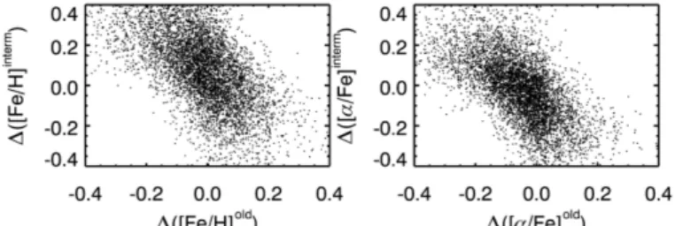
Fig. 7.The dominating degeneracies in the mean light-weighted values when separating SEHs into intermediate and old stars are those between the same properties of the two stellar generations. Each∆ is defined as the recovered minus the true value.
degeneracies, thus these plots are not shown here in the interest of space. However, and as shown in Fig.7, the dominating de-generacies are those between [Fe/H]iand [Fe/H]o and between [α/Fe]iand [α/Fe]o.
At this point we remind the reader of the classification into SLF and ACC galaxies introduced in Sect. 1. Indeed, at spe-cific points in this paper we separate galaxies in two types: 1) Those where [Fe/H]o < [Fe/H]i. For these the [Fe/H] evo-lution with time is consistent with self-enrichment by SNe Ia and these are therefore termed SLF-ETGs (represented by yel-low dots in Figs. 17 to 22 beyel-low). 2) Those galaxies where [Fe/H]o> [Fe/H]i. Those are not consistent with self-enrichment and we infer that some accretion of material must have taken place – whether these were mergers, gas accretion or anything else we remain agnostic about (such as winds redistributing el-ements within a galaxy, see Pipino et al. 2006). Nevertheless, for conciseness we term those merger-accretion or ACC-ETGs (pink color in same figures). A more in-depth discussion of the physical usefulness of this distinction is given in Sect.8.3.
We now explore how robust such a classification would be to degeneracies. Our input mock galaxy catalogue contains 50% SLF and 50% ACC galaxies. After fitting, 81% of the SLF galaxies would be correctly identified but only 33% of the ACC galaxies. Furthermore, after fitting we would identify 74% of the sample as SLF galaxies and 26% as ACC galaxies. Finally, the number that is probably of most interest is the percentage of galaxies in each half of the parameters space that actually is what it pretends to be: The percentage of galaxies that would be classi-fied as SLF galaxies after fitting and that really are SLF galaxies is 55%, while the percentage of galaxies that would be classified as ACC after fitting and that are really ACC galaxies is 65%. While these numbers are sobering, one should remember that they apply to a sample of mock galaxies that completely fills the parameter space available to our models and at a specified S/N of 40. This does not represent the real distribution of galaxies in this parameter space as we shall see below. In particular we shall explore in an observationally motivated way how our con-clusions depend on the exact location of the separation [Fe/H]o< [Fe/H]i + ∆, i.e. how this classification behaves within a range of −0.4 <∆ < 0.4.
Besides direct classification we use another, more statisti-cally minded method to gauge the distribution of observed galax-ies in the planes of [Fe/H]ivs. [Fe/H]o and [α/Fe]ivs. [α/Fe]o, namely the posterior distribution of fitted galaxies. We show the general case in Fig.8: one starting with a uniform distribution of mock galaxies in parameter space. For reasons to be seen later, another interesting case is the one where all galaxies start out in a narrow range of [Fe/H]iand [Fe/H]oabundances. We have cho-sen −0.2 < [Fe/H]i, [Fe/H]o < 0.0. Clearly both cases produce significantly different posterior distributions in parameter space
that can be used to constrain the real distribution of parameters to some extent – or at least can be used to exclude some real parameter distributions.
In this section we have assessed the uncertainties intrinsic to our method under the assumption that the model is a perfect rep-resentation of the data.We have found that these uncertainties exist, but that we can understand, describe and quantify them.
5. Fitting the observed spectra
We now proceed to fit the sample described in Sect.2with the method described in Sect. 4. We did not change the setup of the fitting in any way. This means that we fit the spectra with the same models, the same continuum rectification, and all other parameters being equal. There is only a slight difference in the spectra that may affect the fitting procedure to some extent.
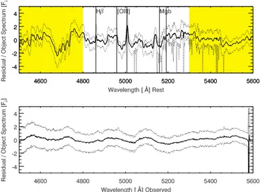
This is seen in the stacked fitting residual vectors of all galax-ies as shown in Fig.9. Our sample has been selected to con-tain emission-line free galaxies as judged byBrinchmann et al.
(2004). However, we find that the residuals do contain emission lines of Hβ and [OIII]. We attribute this finding to our excel-lent stellar population modeling and fitting procedure as well as to conservative estimates of emission line absence. In other words, while to the trained eye emission line residuals in stacked spectra may seem obvious, for an automatic detection procedure it is difficult to attribute a statistical significance to these fea-tures per galaxy, given similar-sized residuals in nearby regions of the spectrum. Emission lines affect only small regions of the spectrum and thus should not affect our overall results. In many cases they are masked away by our automatic outlier rejection in paradise (see AppendixA). We have verified that all our simulation results are independent of the potential missing in-formation in the emission line region by applying an appropriate mask in wavelength space to the mock galaxies and rerunning all simulations. We found no difference in the results.
As a side-note we mention the residual absorption feature around 4700 Å. Its origin is unclear, but it does not affect our measurements as it is outside our fitted wavelength range.
We also investigated the presence of any problems with data quality. Given the precision we are claiming to reach here (not much more than one percent in residual) we might be prone to data quality problems at a level not often seen otherwise. Problems might be present in the SDSS data, but also in the stellar templates. We note, however, that Fig.9does not indi-cate such problems. Indeed, the lower panel shows residuals in the observed frame where data problems such as sky emission line residuals should appear. The only obvious sky residual is at the very red end of the wavelength range shown, but way out-side our fitted wavelength range. A paper dealing in much more detail with template mismatch vs. data quality is in preparation. Another way to assess our fit quality is to compare the cumu-lative histogram of χ2obtained from the spectra in our data with the one expected from statistics, i.e. the χ2-distribution. This is done in Fig.10, assuming 257 degrees of freedom for our fitting procedure, as appropriate after taking into account the number of fitted pixels and the number of free parameters. The distributions do not match perfectly, but they are clearly very similar, both in shape and location. We believe this indicates that the fitting of SDSS spectra is indeed in the realm governed by χ2 statistics, once the models are sophisticated enough and when restricting to a well-known wavelength range.
In Sect.4we used a velocity dispersion of 150 km s−1for all tests, although the velocity dispersion was left a free parameter
Fig. 8.Comparison of the original distribution of parameters (upper row) vs. the one recovered after the fitting process (lower row). We show the two parameter spaces that are of most interest in the remainder of the paper, namely [Fe/H]ivs. [Fe/H]oand [α/Fe]i vs. [α/Fe]o. Left panel: the
case in which the total library of mock galaxies is analyzed. Right panel: the case in which only mock galaxies with −0.2 h [Fe/H]i, [Fe/H]oh 0.0
are analyzed.
Fig. 9.Mean residual vector and its standard deviation from all galaxies
in the sample. The upper plot indicates the residuals in the rest frame of the galaxies, the yellow region has actually not been used to determine the best fit. [OIII] and Hβ emission lines are labelled and clearly visible. The Mgb feature is also indicated for reference, but does not show ev-idence of specific mismatch. The lower plot shows the observed frame residuals indicating no major concern with the data.
in the fitting. Velocity dispersion is clearly different for every ob-served galaxy. We can, however, feed the SDSS pipeline velocity dispersion as a starting value to paradise, thereby essentially mimicking the fact that we know the velocity dispersion for the simulated galaxies. Indeed, we find that we do recover the ve-locity dispersion from the SDSS very well, see Fig.112.
The output of the fitting are tables with all parameters, such as mean light-weighted age ([Fe/H], [α/Fe]) of the entire
2 There is one object out of 2286 where the SDSS pipeline velocity
dis-persion is 224.8 km s−1, whereas paradise determines 118.9 km s−1.
Visually this object clearly has been correctly fitted by paradise. We only have this one example, which however tentatively indicates that velocity dispersion mismatch would not have been a problem for our analysis.
Fig. 10. Cumulative histogram of χ2 values obtained from the data
(solid line) with the χ2distribution expected from statistics (dotted line)
for 257 degrees of freedom.
spectrum, the same parameters only for the “old” stars (i.e. older than 9.5 Gyr) and for the “intermediate-age” stars (i.e. younger than 9.5 Gyr). Typical errorbars on our parameters are 0.2 Gyr on age and 0.01 dex on [α/Fe] and [Fe/H]. These errorbars reflect random errors and degeneracies, but not model-related errors and systematic problems with the recovery. This can be com-pared with the typical errors quoted in one of the classical stud-ies of the field. For definiteness we chooseThomas et al.(2005), without prejudice to later or earlier results. They quote typical er-rors of 1.48 Gyr in age, 0.04 dex in total metallicity, and 0.02 dex in [Fe/H] ratio, although it needs to be said for clarity that these earlier errorbars only take into account the formal uncertainties on the data. Our errorbars also include degeneracies in the stel-lar population mix. In the more recent paper byJohansson et al.
(2012) the uncertainty in [O/Fe] at S/N ∼ 40 in the r-band is given as approximately 0.05 dex, but it needs to be kept in mind that this is the uncertainty on a single element, while we group all α-elements together.
Another important point to mention is that none of the de-rived galaxy ages are older than 13 Gyr, as we show in Sect.6.
Fig. 11.Comparison between the velocity dispersion from SDSS DR7 and those obtained in this work.
While this is predetermined from the range of model spectra in use, there is also no hint of an edge effect in the sense the galax-ies that would be older than 13 Gyr cannot be fitted and there-fore for those galaxies a higher metallicity would be fitted to compensate. We explicitly tested that this edge effect is present if we restrict our template library to SSPs with ages younger than 13 Gyr.
6. Results
We now discuss our findings in terms of correlations between the parameters we determined ourselves, i.e. ages, [Fe/H] and [α/Fe] and those available for our galaxies i.e. stellar mass M* and velocity dispersion σ.
6.1. Theσ-α, M*-α and age-α relations
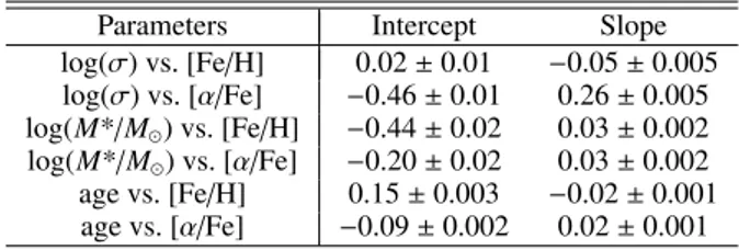
In Fig. 12 we plot [Fe/H] and [α/Fe] versus velocity disper-sion σ, stellar mass M* and mean light-weighted age. We quantify the presence or absence of correlations by means of Spearman rank coefficient tests3 and by means of formal fits
to each set of two parameters combinations using the LINFIT module in IDL. The results of the fits are given in Table1. We confirm correlations between log(σ) as well as log(M*/M ) and [α/Fe] as found in previous work (see Sect.8.1). In Fig.12we also see a strong correlation between age and [α/Fe] as well as [Fe/H] in the sense that [α/Fe] decreases for younger light weighted mean age of the galaxy, while [Fe/H] increases.
There seem to be only weak correlations between [Fe/H] and log(σ). However, Johansson et al. (2012) show that when the sample is decomposed into age bins, each age bin by itself shows a strong correlation with log(σ). In the interest of space we re-frain from repeating the exercise.
Additionally the relation between age and [α/Fe] shows a clear change of slope at age ∼9 Gyr. We have fitted the two regimes separately and find that [α/Fe] = −0.01 ± 0.004 + 0.01 ± 0.001 · age for galaxies younger than 9 Gyr, while
3 The Spearman coefficients measure the strength of a potential
corre-lation, where 0 is no correcorre-lation, 1 is a strong positive correlation and −1 is a strong anti-correlation. The probabilities on the other hand mea-sure the significance of the correlation, i.e. the probability that the real correlation is zero. Therefore a value of 1 for this probability indicates that we know nothing about the real correlation, while a value of below 0.05 would imply that a correlation indeed exists at the 95% confidence level.
Table 1. Correlation strengths for light-weighted mean parameters.
Parameters Intercept Slope
log(σ) vs. [Fe/H] 0.02 ± 0.01 −0.05 ± 0.005 log(σ) vs. [α/Fe] −0.46 ± 0.01 0.26 ± 0.005 log(M*/M ) vs. [Fe/H] −0.44 ± 0.02 0.03 ± 0.002 log(M*/M ) vs. [α/Fe] −0.20 ± 0.02 0.03 ± 0.002 age vs. [Fe/H] 0.15 ± 0.003 −0.02 ± 0.001 age vs. [α/Fe] −0.09 ± 0.002 0.02 ± 0.001 [α/Fe] = −0.20 ± 0.007 + 0.03 ± 0.001 · age for galaxies older than 9 Gyr. For both regimes the probability of the absence of any correlation is zero.
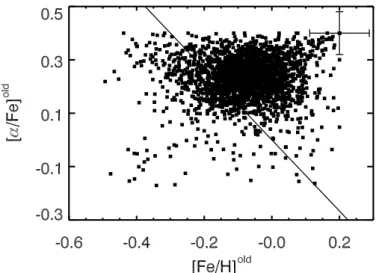
The two rightmost panels of Fig.12already indicate a corre-lation between [α/Fe] and [Fe/H], which we explicitly plot in Fig.13. We find that early-type galaxies all have on average a total metallicity that is roughly solar. It is the ratio between the abundances of Fe and the α-elements that changes between galaxies.
6.2. Separating the old and intermediate components We now show results for resolved SEHs, i.e. looking at the abun-dance ratios of old and intermediate stellar populations sepa-rately. Before we do so, as a cautionary remark, it is worth emphasizing that the uncertainty bars include the uncertainties introduced by the degeneracies characterizing galaxy evolution. Thus a direct visual comparison of the size of the error bar and the scatter in the figures is misleading. The size of the error bar indeed denotes the range of possible values for each sin-gle galaxy. However, on average, galaxies will tend to be as-signed the mean value of that possible range. Scatter in figures is mainly driven by real observational uncertainties and does not represent the degeneracy uncertainties as assessed by paradise. That said, mean uncertainties on our parameters are 0.17 dex for [Fe/H]i, 0.14 dex for [Fe/H]o, 0.12 for [α/Fe]i, and 0.13 for [α/Fe]o.
First we repeat in Fig.14the upper panel of Fig.1, i.e. we show the non-binned average star formation history of all galax-ies in our sample. As this is the observable, we show the star for-mation history in terms of the luminosity contributions of stars of each specified age to the total luminosity of each galaxy. It is noteworthy that several peaks in the star formation history appear, namely at 13 Gyr, 9 Gyr and a somewhat broader one around 6 Gyr. Our SSPs are sampled in steps of 1 Gyr, there-fore intermediate ages could in principle be assigned significant weights by paradise. On one hand it is entirely possible that this is an artifact of our fitting procedure, given that such fea-tures do not appear in the overall star formation history of the universe (Lilly-Madau plot). On the other hand, the two older episodes of star formation seem entirely compatible with the classical two-infall scenario of chemical evolution (Chiappini et al. 1997) that was originally proposed for the Milky Way. Note that these two oldest peaks also contribute to justifying our sep-aration into old and intermediate-age stars at a lookback time of 9.5 Gyr. We come back to this point below when discussing SLF vs. ACC-ETG percentages.
Finally, there is a small peak at less than 1 Gyr which is outside the coverage of our [α/Fe]-enhanced SSP templates. As described in Sect. 3 we include five templates with younger ages, but with solar element ratios only. The total contribution to the light of the population younger than 2 Gyr is however less than 5%. Due to its lower mass to light ratio than the older stellar
Fig. 12.Correlations of [Fe/H] and [α/Fe] with velocity dispersion, stellar mass and mean light-weighted age for our sample galaxies. It is clear that the tightest relations are those with age. Note also the change of slope in the relation between age and [α/Fe] ∼ 9 Gyr. Average error bars are given in the upper right corner of each panel and spearman rank correlation coefficients are also noted.
Fig. 13. Correlation between [Fe/H] vs. [α/Fe] for the luminosity
weighted average properties of the ETGs in our sample. The thick solid line is a line of constant, solar metallicity (Z= 0.017). The two dashed line illustrate the extremes of the ETG locus, i.e. for [Z]= −0.15 and [Z]= 0.18.
populations this translates to an even smaller contribution to the total mass of the galaxy. We thus confirm that ETGs harbor very little young stars – maybe even none, if currently unmodeled old and hot stellar populations indeed do play a role (see e.g.Ocvirk 2010).
It is interesting to start the analysis with plotting the prop-erties of the old stellar populations vs. the global parame-ters of their host galaxies. We refrain from doing so for the intermediate-age populations due to the strong degeneracies we
Fig. 14.Average star formation history of all galaxies in the observed
sample in terms of the present day contribution of each stellar popula-tion to the total luminosity of the galaxy. All galaxies contribute equally to this average, i.e. the total luminosity for each galaxy has been nor-malized to one before averaging.
identified in Sect.4.3 and the lower recovery success for the intermediate component with respect to the old one we identi-fied there. Also, our sample is dominated by galaxies in which the old stellar population contributes more than half of the to-tal light, contributing to possible uncertainties in the properties of the intermediate-age stellar populations. Figure15shows that the correlations seen for the global stellar populations do not hold up for the older stars in the galaxies (compare also Table2). Indeed, while the Spearman rank test indicates a very low prob-ability for the dependence of [α/Fe]o and [Fe/H]o on age to be
Fig. 15.Correlations of the [Fe/H]oand [α/Fe]owith the global properties of the sample galaxies σ, M*, and age. Average error bars are given in
the upper right corner of each panel and spearman rank correlation coefficients are also noted. Table 2. Correlation strengths old stars only.
Parameters Intercept Slope
log(σ) vs. [Fe/H]o −0.73 ± 0.046 0.29 ± 0.020 log(σ) vs. [α/Fe]o 0.37 ± 0.046 −0.05 ± 0.020 log(M*/M ) vs. [Fe/H]o −0.83 ± 0.066 0.07 ± 0.006 log(M*/M ) vs. [α/Fe]o 0.46 ± 0.063 −0.02 ± 0.006 age vs. [Fe/H]o 0.13 ± 0.013 −0.02 ± 0.001 age vs. [α/Fe]o 0.39 ± 0.012 −0.01 ± 0.001
spurious, inspection of the plot tells another story. There is a cloud of points at older ages, while the galaxies with younger ages show much larger scatter. This can be understood as be-ing caused by difficulties in accurately estimating [α/Fe]o and [Fe/H]o for galaxies with significant intermediate-age popula-tions. We therefore attach no importance to these relapopula-tions. For σ and M* vs. [α/Fe]o, the Spearman test indicates weak correlation and indicates a high probability (0.68) of no correlation for M* vs. [α/Fe]o. We are thus left with the indication that [Fe/H]o de-pends positively on mass as parameterized by either σ or M*, but more strongly on the former. This correlation is driven mainly by the presence of objects with low [Fe/H]o at low σ values. Overall these trends are opposite to the average properties, where [α/Fe] depends clearly on mass and [Fe/H] does not.
The two rightmost panels of Fig.15already indicate that the correlation between [α/Fe] and [Fe/H] that is valid on average for early-type galaxies does not hold up when considering the old stars only. Indeed, in Fig.16we find that old stars in early-type galaxies have on average super-solar metallicity, where both [Fe/H]o and [α/Fe]o are super-solar. That these properties seem to be independent of mass (see Fig.15) might be one of the most puzzling findings of this paper.
Fig. 16.Relation between [Fe/H]ovs. [α/Fe]o, the thick line is a line of
constant, solar metallicity (Z= 0.017). This is the same as Fig.13, but only for the stars older than 9.5 Gyr in each galaxy. The old stars in early-type galaxies, have on average high total metallicity, significantly super-solar. Average error bars are shown in the upper right corner.
6.3. Exploring the possible dichotomy SLF vs. ACC
In Fig. 17 we show the distribution of [Fe/H] and [α/Fe] of the intermediate vs. the old component (left panels). In [Fe/H] galaxies can lie both above the identity line and below it. In [α/Fe], almost all galaxies lie below the identity line, with a few slight outliers that can be thought of as being due to un-certainties. When looking back at Fig.8 and the discussion in Sect. 4.3, it is obvious that any statement on the distribution in these panels must take into account the uncertainties due to
Fig. 17.Left panels: distribution of mean light-weighted [Fe/H] and [α/Fe] for the old vs. intermediate sub-populations. Galaxies in yellow are
those where [Fe/H]o < [Fe/H]i−0.15 (SLF-ETGs), pink where [Fe/H]o> [Fe/H]i+0.15 (ACC-ETGs). Galaxies with uncertain classification are
shown in black. Average uncertainties including all degeneracies are shown in the upper left corners. Right panels: age dependence of [Fe/H] and [α/Fe] within each galaxy, i.e. their enrichment history. Galaxies with uncertain classification have been omitted for clarity.
the degeneracies in properties between old and intermediate-age stars. In turns out it is easier to discuss the results in terms of what the data are incompatible with and this is what we do.
The distribution of points in the upper left panel on Fig.17
is incompatible with a flat distribution in that plane. I.e. early-type galaxies do not have a random distribution of [Fe/H]iand [Fe/H]o. Rather their distribution is more similar to the right pan-els in Fig.8, where the underlying sample had a narrow distri-bution of [Fe/H]iand [Fe/H]ocentered around −0.1 for both.
The distribution of points in the lower left panel of Fig.17
is equally incompatible with a flat distribution in that plane. I.e. early-type galaxies do not show a random distribution of [α/Fe]i and [α/Fe]o. It seems rather secure that the oldest gen-eration of stars has a high [α/Fe] ratio, higher than 0.1, whereas the intermediate-age stars have a lower ratio of [α/Fe], certainly below 0.1 and going as low as our model permits, i.e. −0.2. Note that [α/Fe] values below zero for late stellar generations are a generic prediction of chemical evolution models in mas-sive galaxies ([Fe/H] Minchev et al. 2013, their Fig. 5). On the other hand low-mass galaxies do not necessarily show low [α/Fe].Recchi et al.(2001) for example show that stellar winds tend to carry elements produced by SNeIa away, thus leaving behind gas with higher [α/Fe] than expected from the extent of their SFH.
Coming back to the distinction discussed in Sect. 4.3 be-tween ETGs that are compatible with self-enrichment (SLF-ETGs) and mergers/accretion (ACC-ETGs), we wish to identify galaxies that we can reasonable safely assign to any of these cat-egories. SLF-ETGs are those where [Fe/H]o < [Fe/H]i–∆, and ACC-ETGs are those where [Fe/H]o> [Fe/H]i+ ∆. Motivated by the sizes of the error bars quoted in the beginning of Sect.6.2and after some testing in the simulations, for definiteness we choose ∆ = 0.15. Our results qualitatively do not depend on the exact size of∆4. We emphasize that this choice of∆ also mitigates
concerns over the subtle drop in metallicity at late times shown in the paper byVazdekis et al.(1996) and discussed in the intro-duction. We call the remaining galaxies that are neither one nor the other the “gray-ETGs”. Note that for the observational re-sults we include into the class of “gray” galaxies those galaxies that have less than 15% of light in either the old or intermediate stellar populations. This is to account for possible uncertainties in stellar population modeling and in the fitting algorithm.
For the sample of 2286 galaxies analyzed here we find that 29% belong to the ACC-ETG class. 63% are unclassifiable, but
4 For this∆ and for the simulations, the percentage of galaxies
identi-fied as ACC-ETGs after the fitting process, which are truly ACC-ETGs is 77%. The percentage of galaxies identified as SLF-ETGs after the fitting process, which are truly SLF-ETGs is 63%.
Fig. 18.Correlations of [Fe/H] and [α/Fe] with velocity dispersion, stellar mass and mean light-weighted age for our sample galaxies (same as Fig.12). Colors reproduce the classification from Fig.17into SLF-ETGs (yellow) and ACC-ETGs (pink). The mean for each subpopulation is also shown as a large square with black borders. Galaxies that could not be reliably classified are shown as black dots.
most of those would be called ACC-ETGs as well if not for the requirement to have 15% of light at least in the intermediate-age population. Only 8% of the galaxies are bona-fide SLF-ETGs, i.e. consistent with a self-enriching star formation history.
We caution that effects of degeneracies between the proper-ties of the intermediate and old stellar populations, sample selec-tion effects, the uncertainty on the exact boundary to be applied between old and intermediate stellar populations, specific effects of chemical evolution such as the drop in metallicity for young stars in massive ETGs, all contribute to make these numbers in-dicative only. To indicate the possible size of changes due to at least one of these effects we have recomputed the percentages of SLF and ACC-ETGs for a choice of 8.5 Gyr as the bound-ary between old and intermediate-age ETGs. We find that this inverts their relative importance, i.e. 30% of the sample would then be SLF ETGs, while only 3% bona-fide ACC-ETGs remain. This high sensitivity of the results to the adopted age boundary is due to a very low [Fe/H] abundance attributed by the fitting code to the spike in the SFH at 9 Gyr. This significantly low-ers the average [Fe/H]oabundance, thus increasing the number of SLF-ETGs.
Given the magnitude of this effect, we have to carefully state our arguments for choosing 9.5 Gyr lookback time as our boundary. Indeed, we have argued in the introduction on physi-cal grounds that 9.5 Gyr is a more physiphysi-cal boundary. On techni-cal grounds, we refer to Fig.14which shows that the 9 Gyr age bin in the finely sampled SEH has a close significant neighbor-ing age bin at younger age (7 Gyr), while the next significant old age bin (at 13 Gyr) is more distant in look-back time. Generally speaking, it is clear that there are significant degeneracies be-tween the properties of adjacent bins in the reconstructed SEH. We have shown the extent of these degeneracies in Fig. 7 for the coarsest possible choice of SEH, namely an SEH with two
age bins. Degeneracies only increase for an SEH with a finer age grid. Degeneracies between the 7 and 9 Gyr age bins shown in Fig.14are therefore much more likely than between the 9 and 13 Gyr age bins. This is the technical reason why we believe the results based on a 9.5 Gyr boundary to be more reliable and sig-nificant than those we would have obtained based on any other boundary.
Figure18repeats Fig.12but adding the information about the enrichment history classification. It is immediately clear that on average and for our sample ACC-ETGs are significantly older than SLF-ETGs (compare also Fig.25). Also, on average SLF-ETGs have lower velocity dispersion and lower [α/Fe] than ACC-ETGs. We come back to these features in the discussion Sect.8.
6.4. Environment
While nearly out of the focus of this paper, environment is such an important parameter for galaxy evolution that it would be foolish to leave it entirely out. Much work has been done on assessing the correlations between environment and the proper-ties of early-type galaxies and we do not wish to simply repeat this work here, as we strongly expect to confirm it. Rather, in the interest of space, we concentrate only on the correlation of the old stellar population properties [Fe/H]oand [α/Fe]owith en-vironment, taking into account our classification in ACC-ETGs and SLF-ETGs. We are particularly interested to see whether the initial star formation event indeed depends on environment ([Fe/H] Renzini 2006).
As a measure of environmental density we use the one by
Tempel et al.(2012), specifically we use the density as derived within 8 Mpc, i.e. their parameter dens8. Their densities are based on luminosity densities around each galaxy calculated in
Fig. 19. Environmental density vs. light-weighted [Fe/H] and [α/Fe]
(upper panels) and vs. [Fe/H]oand [α/Fe]oof only the old stars in each
galaxy. The mean for each subpopulation is also shown as a large square with black borders.
three coordinates, i.e. two projected spatial distances and one based on redshift, the latter however including advanced tech-niques to suppress peculiar motions such as suppression of the finger-of-god effect. We refer to the original paper for all the details.
Perhaps surprisingly we find in Fig.19that the old stellar population may not be affected by environment. This is clearly different from what other authors found for the entire galaxies (Sánchez-Blázquez et al. 2006). It however agrees with infer-ences made inThomas et al.(2010). These authors discuss that ETG formation has occurred in two phases, where ETG galaxy formation depended on mass only and not on environment.
Rettura et al.(2010) on the other hand argue that while the en-vironment may modulate the timescale of the star formation his-tory for ETGs, the formation epoch is essentially independent of environment and seems to depend on mass only. We here add another piece to the puzzle in saying that for the oldest stars in each galaxy, older than 9.5 Gyr, galaxy formation seems to have been independent of mass and environment, at least for the mass range probed here.
7. Aperture effects
As discussed in Sect. 1, the cores and the envelopes of ETGs may have assembled in different ways and at different times. Also, winds can redistribute elements within a galaxy (Pipino et al. 2009). Observationally, gradients in element abundances are observed for galaxies in general ([Fe/H] Sánchez et al. 2013;
Pérez et al. 2013). However, for ETGs the gradients in age and [α/Fe] are observed to be small or null on average (Mehlert et al. 2003;Rawle et al. 2008;Kuntschner et al. 2010). Not so for the gradient in [Fe/H], which can be significant ([Fe/H] Spolaor et al. 2008). The SDSS uses a single fiber to observe the centers of the target galaxies. The fibers fixed aperture on the sky (300) covers a different fraction of the target galaxy, depending on its intrinsic size and redshift. This effect is somewhat counteracted by the effects of seeing, as seeing will also scatter light from larger radii into the fiber area in the focal plane. It is neverthe-less clearly important to assess this covering fraction and the potential impact on our results. Proper aperture corrections as demonstrated in Gallazzi et al. (2008) is beyond the scope of the present paper. We also refer to the discussion inChoi et al.
(2014) for another angle on the same question, albeit they work on a larger redshift range.
Fig. 20.Dependence of key physical properties of our sample galaxies
on redshift. From top to bottom: stellar mass, [α/Fe], age and ratio be-tween radius covered by fiber and effective radius of the galaxy. Colors reproduce the classification from Fig.17into SLF-ETGs (yellow) and ACC-ETGs (pink).
Figure20shows the dependence of key physical properties on redshift for our sample. In the uppermost panel the effects of apparent magnitude selection are obvious in that we sam-ple more massive objects at larger distances from Apache Point Observatory. The next panel shows the dependence of the cov-ering fraction on redshift in terms of the ratio between the fiber size and the galaxies effective radius. We use the effective radius from the SDSS pipeline surface brightness profile fit with a de Vaucouleurs profile. It illustrates that two effects nearly cancel each other: on the one hand, the higher the redshift, the larger the area covered by a fiber is physically smaller on the galaxy. On the other hand, the galaxy itself will tend to be more massive and therefore larger. The covering fraction thus depends less on redshift than the stellar mass. The next panel shows the expected non-dependence of [α/Fe] on redshift, given that [α/Fe] varies little with mass and galaxies have flat gradients if any. The final panel shows that [Fe/H] depends in an interesting way on red-shift. Because of the stronger gradients and stronger dependence of [Fe/H] on mass it is nontrivial and beyond the scope of the present paper to understand this.
The crucial test, however, is shown in Fig. 21, where we show the dependence of [Fe/H] on covering fraction at a fixed mass (here chosen to be 10.5 < log (stellar mass/M ) < 11.0). There is no obvious bias to be seen, besides a potentially spuri-ous tendency to have less [Fe/H]-rich objects at larger covering fraction. We conclude that tests on possible aperture biases are not conclusive enough to endanger any of the fairly general con-clusions of this paper.
Any further investigation of aperture effects, in particular as concerning the resolved SEHs, i.e. the potentially different bi-ases on the old and intermediate-age stars) will have to await analysis of the currently on going integral field spectroscopy sur-veys such as CALIFA (Sánchez et al. 2012), SAMI (Allen et al. 2015), and Manga (Bundy et al. 2015).
8. Discussion
8.1. Comparison of average quantities to earlier observational work
A simple test is to situate our galaxies on the stellar mass – stel-lar metallicity relation as defined byGallazzi et al.(2005) and
![Fig. 1. Schematic representation of the new parameters introduced in this paper, namely [α/Fe] o and [Fe/H] o](https://thumb-eu.123doks.com/thumbv2/123dokorg/8091912.124679/3.892.462.820.111.575/fig-schematic-representation-new-parameters-introduced-paper-fe.webp)
![Fig. 13. Correlation between [Fe/H] vs. [α/Fe] for the luminosity weighted average properties of the ETGs in our sample](https://thumb-eu.123doks.com/thumbv2/123dokorg/8091912.124679/11.892.59.836.612.899/fig-correlation-luminosity-weighted-average-properties-etgs-sample.webp)
![Fig. 17. Left panels: distribution of mean light-weighted [Fe/H] and [α/Fe] for the old vs](https://thumb-eu.123doks.com/thumbv2/123dokorg/8091912.124679/13.892.64.832.95.665/fig-left-panels-distribution-mean-light-weighted-fe.webp)
