A
A
l
l
m
m
a
a
M
M
a
a
t
t
e
e
r
r
S
S
t
t
u
u
d
d
i
i
o
o
r
r
u
u
m
m
–
–
U
U
n
n
i
i
v
v
e
e
r
r
s
s
i
i
t
t
à
à
d
d
i
i
B
B
o
o
l
l
o
o
g
g
n
n
a
a
DOTTORATO DI RICERCA IN
Biodiversità ed Evoluzione
Ciclo XXIV
Settore Concorsuale di afferenza:
05/B1 – Zoologia e Antropologia
TITOLO TESI
E
E
c
c
o
o
l
l
o
o
g
g
i
i
c
c
a
a
l
l
g
g
e
e
n
n
e
e
t
t
i
i
c
c
s
s
a
a
n
n
d
d
c
c
o
o
n
n
s
s
e
e
r
r
v
v
a
a
t
t
i
i
o
o
n
n
g
g
e
e
n
n
o
o
m
m
i
i
c
c
s
s
o
o
f
f
w
w
o
o
l
l
f
f
(
(
C
C
a
a
n
n
i
i
s
s
l
l
u
u
p
p
u
u
s)
s
)
Presentata da: Marco Galaverni
Coordinatore Dottorato
Relatore
Barbara Mantovani
Ettore Randi
E
E
c
c
o
o
l
l
o
o
g
g
i
i
c
c
a
a
l
l
g
g
e
e
n
n
e
e
t
t
i
i
c
c
s
s
a
a
n
n
d
d
c
c
o
o
n
n
s
s
e
e
r
r
v
v
a
a
t
t
i
i
o
o
n
n
g
g
e
e
n
n
o
o
m
m
i
i
c
c
s
s
o
o
f
f
w
w
o
o
l
l
f
f
(
(
C
C
a
a
n
n
i
i
s
s
l
l
u
u
p
p
u
u
s)
s
)
From the Major Histocompatibility Complex to the first wolf genome draft(and some secrets of dog domestication)
“The greatest danger for most of us is not that our aim is too high and we miss it, but that it is too low and we reach it”
Summary
1. Introduction
1.1. Overview on a fast-changing scientific era
1.2. From Population Genetics to Ecological Genetics and Conservation
Genomics
1.2.1. New perspectives
1.2.2. New technologies: Next Generation Sequencing
1.3. The species: Canis lupus, Linnaeus 1758
1.3.1. Origin and distribution
1.3.2. Morphology and biology
1.3.3. Threats and legal status
2. The Major Histocompatibility Complex: its variability in the Italian wolf
population and its influence on mating choice and fitness traits
2.1. Background
2.1.1. Structure and functions
2.1.2. Genetic features and evolution
2.1.3. Methods
2.1.4. Studies
2.1.5. MHC in canids
2.2. Aims
2.3. Methods
2.4. Results
2.5. Discussion and implications
3. The first wolf genome project
3.1. Background
3.1.1. Overview on whole-genome studies
3.1.2. The dog genome
3.1.3. Dog domestication and breeding
3.2. Aims
3.3. Methods
3.3.1. Sequencing methods
3.3.2. Analyses workflow
3.4. Preliminary results
3.5. Discussion and implications
4. Conclusions
5. Bibliography
1. Introduction
1.1. Overview on a fast-changing scientific era
A very few fields in research have seen such a fast evolving phase in the recent years as genetics.
As a beginning researcher, I am astonished in seeing the rhythm of new techniques, approaches and questions arising during just the few months of my doctoral project.
But on the other side, this cultural blast offers great opportunities for those who are interested (and so am I) in following the wave, or riding it, and looking for the thousand possibilities of applying the results of research to the widest range of applications.
In this dissertation, we will try to have a closer look at the fields of Ecological Genetics and of the brand-new Conservation Genomics, using as a study species one of the most fascinating carnivores ever appeared on Earth: the wolf.
1.2. From Population Genetics to Ecological Genetics and Conservation
Genomics
The past decade has seen a large usage of neutral-behaving genetic markers such as microsatellites (or single tandem repeats, STRs) and mitochondrial DNA (mtDNA) control region, in order to assess the basic genetic variables in animal and plant populations, with particular attention to the ones presenting conservation concerns (Ouborg et al. 2010).
Those estimates have allowed to identify cases of reduced effective population size, restricted gene flow, limited heterozygosity, but also inbreeding, past bottlenecks and hybridization or gene introgression, all factors that could seriously affect the population viability and long-term survival, especially in times of fast climate changes and strong human-driven environment modifications.
The same genetic markers allowed the researchers to reconstruct the phylogenetic relationship, social structure, kin affiliations and individual fitness estimates in many social species, particularly among mammals and birds.
Nonetheless, new questions are arising on the shoulders of the previous ones, and their answers are now much closer also thanks to great technological improvements occurred in the last years, and to the analytical tools related to them.
Figure 1: network of interacting factors that can be addressed by conservation genetics (blue) and genomics (red). (From Allendorf et al. 2010)
1.2.1. New perspectives
Ecological Genetics, or Molecular Ecology, is not a new research field.
The study of the relationships of individuals with the environment (represented both by the habitat, the social structure, the food networks -especially the prey-predator relations and co-evolution- the climate and the pathogens), based on their genetic background, and the returning effects of the environment in driving and shaping the genetic features of the individuals through natural and sexual selection, has seen a never-dropping interest.
However, the limited resources usually available to researchers did not allow for the investigation of a large number of genetic markers, therefore often limited to a few genes or non-coding regions of interest.
Nowadays, on the contrary, revolutionary technologies allow for the screening of thousands of genome-wide genetic markers, e.g. single nucleotide polymorphisms (SNPs), or, moreover, whole genome sequences in a very short time and a relatively limited economic effort.
This huge upgrade can make it easier to deepen existing disciplines (as for Ecological Genetics -or Molecular Ecology- and Genome-Wide Association Studies -GWAS), thanks to the enlargement of the number and size of the markers, or even to open the way to the development of new branches, such as Conservation Genomics (Ouborg et al. 2010).
This emerging discipline can be simply defined as the application “of new genetic techniques to solve problems in conservation biology” (Allendorf et al. 2010), such as genetic drift, hybridization, inbreeding or outbreeding depression, natural selection, loss of adaptive variation and fitness (Fig. 1).
The whole genomes of some endangered species have been recently completed, starting from the Great Apes: chimpanzee, gorilla and orang-utan (Locke et al. 2011); however, these data will not automatically provide useful data for their conservation (Frankham 2010), especially given the limited information about population variation that we are able to deduce from single individual sequencing. Nonetheless, this will provide a great aid in identifying genetic markers that can be applied to the study of entire populations (Frankham 2010).
Genomic information will turn out to be useful also to try and recover populations from strong inbreeding depressions, by identifying the genes exposing deleterious alleles (Allendorf et al. 2010) and augmenting the population variability with crosses of the most appropriate individuals (Frankham 2010). On the other side, the same techniques will allow to identify the loci most responsible for speciation or cryptic local adaptation, or for exposing populations to severe diseases (Allendorf et al. 2010), such as the facial tumor affecting the Tasmanian devil or the fungus threatening several bat populations.
Having a minor focus on conservation issues, other disciplines (whose limits are often difficult to distinguish) raised, such as evolutionary and ecological functional genomics (EEFG; Feder and Mitchell-Olds 2003).
Meanwhile, international consortia such as the 1000 Genomes Project are already aiming at sequencing a population-wide sample of genomes “to provide a deep characterization of [human] genome sequence variation as a foundation for investigating the relationship between genotype and phenotype” (The 1000 Genomes Project Consortium 2010). Moreover, an even more ambitious project, the Genome 10Kproject (http://www.genome10k.org/), aims at collecting a whole genomic zoo, including thousands vertebrate species from different genera (Genome 10K Community of Scientists 2009).
However, beside this unique kind of projects, the full sequencing of a de novo transcriptome or genome, even in non-model eukaryotic species, is becoming feasible for most of the research institutions.
In the next paragraph, we will see some details that are common to most of the state-of-the-art sequencing platforms, usually indicated as Next Generation Sequencing, that make all the mentioned projects and applications possible.
1.2.2. New technologies: Next Generation Sequencing
Big revolutions often start from very simple ideas that quickly constitute new paradigms. In our case, the simple idea behind a new generation of sequencing techniques is the passage from a single sequencing reaction and reading (usually capillary-based, ‘Sanger’ method) to a multiple, parallel process involving thousands of fragments.
And as in many other fields, often a plethora of similar developments takes place in a very short time and along independent paths, giving place to a number of platforms addressing the same targets in slightly different ways.
However, although in order to highlight the terrific improvements in the sequencing capacity they have been defined as Next Generation Sequencing (NGS) techniques, their immediate diffusion and application should better let us define them as This Generation Sequencing. And their costs, that on a per-base scale are dropping constantly, will soon make them available to an increasingly larger community of investigators in many fields other than human medical research.
The methods
As we just saw, a number of different technologies have been developed in order to achieve similar goals. Nonetheless, the sample preparation and the sequencing methods show a common framework, namely the ability of processing millions of short fragments (also defined as ‘reads’) at the same time, on the same instrument, in the same run (the so-called ‘in parallel’ sequencing).
The starting point (Mardis 2008) is to build a set of fragments (usually named ‘library’) that does not require the cloning by any bacterial vector. These libraries are produced by a mechanical or enzymatic fragmentation of the whole DNA of the target organism or cells. The fragments with the desired length are selected, ligated to oligonucleotide probes (‘adaptors’) and amplified. The nucleotide sequence of every fragment clone is then fixed on a support, read in parallel through a chemical -usually base-by-base- process, and digitalized. However, every company has developed a unique system based on different techniques. In the next paragraph, we will see the protocols and instruments adopted by the three major companies that nowadays compete for the largest part of the Next Gen Sequencing market.
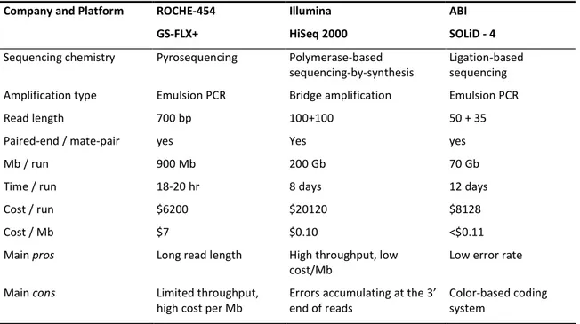
The major platforms: Roche-454 GS, Illumina HiSeq, ABI SOLiD.
When comparing sequencing systems, there are a number of factors to be considered (Cokus 2011). First of all, two quantitative measures, namely the total quantity of sequence (‘throughput’) and the average size of each fragment (‘read length’). Secondarily, but with a comparable importance, the quality of the output, represented by the type and frequency (‘error rate’) of the errors, the reproducibility of the output, and the random sampling of the molecules. Beside these, other important factors are the running time (it matters when it comes from hours to weeks!) and the number of runs that can be performed at the same time, but also the simplicity of the sample preparation (in terms of flexibility, quantity of DNA required, and number of libraries that can be pooled in the same run) and the analysis pipeline (comprehensive of the hardware needed, software power and availability, people and expertise needed for managing it). Eventually, but probably the most important, the costs, which should be carefully considered, including the expenses for buying the instrument, its maintenance and depreciation, the reagents and the ordering quantities.
When considering all of this, even for large institutions, outsourcing to a service company can sometimes turn out to be the most affordable solution: in this case, only the costs per sequencing run and per Mb produced have to be weighted to the scale of the project we are interested in performing.
One of the very first platforms to be developed and successfully applied to a number of studies has been produced by Roche-454 and commercialized in 2004. Named GS Sequencer (with different editions that appeared through years, such as FLX), is based on a pyrosequencing reaction. The amplification step occurs in an emulsion PCR, where the fragments are ligated to agarose beads thanks to universal adaptors and amplified in an oil-water mixture, in which every oil-water-phase drop contains a single DNA fragment and all the amplification reagents. Every bead-linked clone is then located in a unique, picometer-sized well on the surface of a titer plate (PTM). Nucleotides and pyrosequencing reagents are then added in cycles, and the light emission caused by the luciferase during the incorporation of a given nucleotide allows the imaging of the sequence as a flowgram, where the intensity of the light is proportional to the number of nucleotides with the same base that have been incorporated consecutively. Therefore, the length of homopolymers is the limiting factor in the accuracy of the machine. Conversely, the long read length allowed by the pyrosequencing approach, compared to the other platforms, is the main advantage of the system (Tab. 1).
Company and Platform ROCHE-454 GS-FLX+ Illumina HiSeq 2000 ABI SOLiD - 4
Sequencing chemistry Pyrosequencing Polymerase-based
sequencing-by-synthesis
Ligation-based sequencing
Amplification type Emulsion PCR Bridge amplification Emulsion PCR
Read length 700 bp 100+100 50 + 35
Paired-end / mate-pair yes Yes yes
Mb / run 900 Mb 200 Gb 70 Gb
Time / run 18-20 hr 8 days 12 days
Cost / run $6200 $20120 $8128
Cost / Mb $7 $0.10 <$0.11
Main pros Long read length High throughput, low
cost/Mb
Low error rate
Main cons Limited throughput,
high cost per Mb
Errors accumulating at the 3’ end of reads
Color-based coding system
Table 1: Summary of the sequencing approaches and specifications offered to date by the three most common platforms (modified from Mardis 2008 and from Glenn 2011).
The approach followed by Illumina (former Solexa) since 2006, both in the first-born
Genome Analyzer and in the current HiSeq platforms, is based on the so-called
sequencing-by-synthesis (SBS) process. The single-strand DNA fragments are ligated at both ends to the internal surface of a glass cell (divided into eight lanes) thanks to oligonucleotide adaptors that bind complementary probes attached to the cell, forming a bridge-like structure. The fragments are then provided the amplification reagents and incubated, forming clonal clusters randomly located on the cell surface. In the sequencer, in the reads of every cluster the polymerase incorporates a single fluorescent nucleotide of the four provided at every cycle, which also carries a 3’-OH group in order to immediately terminate the extension and to be read by an imaging device. After every incorporation, the OH and the fluorochrome groups need to be removed before the starting of a new cycle. The time required for every step is therefore the limiting factor determining the read length, whereas the problem of homopolymer reading is strongly reduced compared to 454 (Tab. 1).
Also Applied Biosystems in 2007 developed its own platform, named SOLiD in order to designate the “Sequencing by Oligo Ligation and Detection” process used and the proclaimed accuracy of the machine. The amplification step follows an emulsion-PCR reaction where the DNA fragments are added an adaptor and ligated to magnetic beads by complementary oligos. The bead complexes are then fixed to a glass slide for the sequencing step, in which a set of semi-degenerated 8mer probes hybridize to the DNA fragments starting
from a primer annealed to the know adaptor sequence, every probe interrogating two positions, whose nucleotides combination is signalled by a specific fluorochrome on the probe. The fluorescent group is then removed, allowing the ligation of the following probe that will interrogate other two nucleotides 5 bp apart from the first ones, and so on until the end of the fragment. The whole cycle is repeated five times starting from different points (n, n-1, n-1, n, n-1) defined by distinct primers, permitting the reading of the whole fragment twice. The next step is deciphering the 2-bp code, starting from the know adaptor, that will be represented by a sequence of colors. This allows the discrimination of sequence differences (SNPs) from sequencing errors, therefore increasing the accuracy at the price of short reads and long running time (Tab. 1), but with a total throughput nonetheless many times higher than by 454.
However, beside these three main competitors, a range of new companies are emerging and developing -sometimes radically- new techniques that in the next few years could revolutionize the field, and potentially also the geography, of genomic research.
The emerging platforms
A revolutionary approach (D. J. Turner et al. 2009) was presented by the Helicos true single-molecule-sequencing (tSMS) technology, which does not require any amplification step before the sequencing (Braslavsky et al. 2003), therefore avoiding PCR-induced biases (CG content bias, phasing errors). It allows for the extension of about 800M of short (25-50 bp) fragments ligated by a poly-A tail to complementary poly-T adaptors on the cell surface. Then the sequences are read by adding single fluorescent nucleotides in a pyrosequencing fashion. Similarly to 454 instruments, it shows accuracy problems with long homopolymer sequences. The error rates can be reduced by reading the same fragments twice, but also increasing the costs, which can turn out to be already a limiting factor.
Another single-molecule reading platform is represented by the Pacific Bioscience
SMRT (Eid et al. 2009), which is based upon the use of nucleotides labeled with reversible
fluorophores that can be sequentially inserted by a single polymerase inside a nano-sized pore (‘smart cell’); afterward their fluorescence can be read by contrast to the background noise (the so-called ‘Zero mode waveguides’). It can produce an output of only ca. 40 Mb per run, but it is fast, cheap and the reads are longer than in many other platforms, although the same fragment should be read multiple times in order to get a satisfactorily low error rate.
Oxford Nanopore BASE platform, currently hold by Illumina, is also based on a single-molecule approach (Maglia et al. 2008). The fragment sequence is deduced by the
conductivity changes perceived when a nucleotide, after being digested by an exonuclease, passes through a nanopore and binds to a cyclodextrin. The nanopores are placed into a double lipid layer onto a microwell hosted on a silicon chip.
The IonTorrent (Life) system has been incorporated by the ABI company, and also promises to be among the most competitive platforms on the market also thanks to the very limited size. The system is based on a sequencing-by-synthesis reaction on a silicon chip, where the incorporated nucleotides are read by nanoscopic pHmeters, rather then by camera; it can produce about 1Gb of output sequence in a simple and fast way.
Alternative approaches can be represented, for instance, by a ‘strobe’ sequencing, where 50 bp fragments are sequenced every 10 kb along the genome, allowing an optimal reconstruction of structural variants. In the future, the so-called “physical methods” will not require the use of any biological enzyme, but will be based on the physical properties of the DNA molecule itself, such as the different electrical signal produced by the nucleotides (Reveo), possibly read on a ‘DNA transistor’ (IBM). But this is the future, and their commercial production is still to come (see Glenn 2011 for an exhaustive review).
Whatever the platform, the exponential growth of the sequencing power will probably allow us to sequence millions of genomes in the next decade. But -beside strong information storage issues- the next problem will be: what to do with them?
The applications
Multiple studies have exploited the possibilities offered by the NGS platforms, and they can be grouped into three main categories based on their target information: DNA sequencing, RNA-based studies and, recently, methylome sequencing.
The first group is mainly represented by whole genome sequencing studies, in which the candidate genome is sequenced up to a sufficient coverage to allow its complete reading. Whereas this can be relatively simple for the less complex genomes, such as prokaryotes, the studies on animal and plant species are still relatively few. This approach is usually followed when the reference genome of a close relative species is not available, therefore is not possible to apply the same markers (e.g. known SNPs) to study of the target species. For the same reason, it usually requires a de novo assembly process, that can be time-consuming and difficult in the case of complex genomes, such as for polyploid plants. However, even the complete sequencing of a single individual usually allows the detection of millions of Single Nucleotide Variants (SNVs), that can be then used at a population level as markers, for example, in Genome-Wide Association Studies (GWAS) or in population genetics, and other
markers such as microsatellites (STRs) can be identified. If the coverage produced by the chosen platform is sufficiently high and the library preparation requirements allow it, more than one individual can be pooled on the same run. In this way, by comparing multiple genome, a higher number of SNVs and a list of genomic structural features, such as Structural Variants (SVs) and Copy Number Polymorphisms or Variants (CNVs) can also be detected, in addition to insertions and deletions (InDels) events, which are usually linked to repetitive and mobile elements (e.g. Short or Long Interspersed Elements, SINEs and LINEs).
Other members of this DNA-sequencing category are represented by several approaches of targeted sequencing (or re-sequencing): in these cases, only a portion of the candidate genome is selected and sequenced, in order to focus the efforts on a given set of regions of interest. The tools that allow the selection of genomic subsets are several, and they mainly include: Reduced Representation Libraries (RRLs, Altshuler et al. 2000); commercial or custom Targeted Capture arrays (Hodges et al. 2009); Complexity Reduction tools (CRoPS, van Orsouw et al. 2007). These approaches have been successfully applied to the study of large genomes (Burbano et al. 2010, Ng et al. 2009, Wiedmann et al. 2008), although capture arrays require the prior knowledge of the target sequence -or at least the one from a similar organism.
Intermediate between DNA and RNA sequencing approaches we find the transcriptome sequencing (also called mRNA-seq). Beside the fact that works with messenger RNA (mRNA) as starting material (then reverse-transcribed into cDNA), it is basically another way of focusing the sequencing efforts on a subset of the genome, namely its codifying portion: the exome. Its main advantages are that it allows to reach a much higher coverage at a much lower cost, since the size of the protein-coding elements is usually a small fraction of the total genome (ca. 1% in humans, Ng et al. 2009), it does not include complex structural features (such as repetitive elements) and the markers identified from it can be directly related to their possible biological function. If the read length and the coverage are sufficiently high (hundreds of bases) a self-assembly could be achieved without unsolvable nodes, therefore making these studies feasible even in absence of a reference genome.
The second group, including gene expression studies, directs its aim at evaluating which genes are expressed and the differences in the expression levels of the transcripts, usually by comparing multiple individuals of the same species or by pooling individuals from different groups to be contrasted. Also in this case, the mRNA is first selected out of the total RNA, then retro-transcribed into cDNA. The reads are usually aligned to reference genomes, or directly to other reference mRNAs. However, if the reads are sufficiently long to allow the
unique identification of the transcript they match to, they can be directly used for the quantification of the gene expression without the need of assembly them. However, the expression levels of the genes can vary by orders of magnitude, even from tissue to tissue, therefore requiring coverage much higher than for standard sequencing. Many of the pioneering studies (a few years ago, though) were based on the Expressed Sequence Tags (ESTs), an approach that allows to sequence only the terminal portions of each transcript, therefore saving precious sequencing power at the cost of loosing sequence information at the central part of the transcripts. mRNA-seq can be an important step in the annotation of the genes.
The third group, although less common than the previous ones in the scientific literature, is addressing questions on the methylation status of candidate genomes, allowing to focus on some of the main features influencing the epigenetic regulation (Bossdorf et al. 2008). Briefly, it is based on the detection of the differences between the cytosine carrying a -CH3 group (which can be turned into thymine if treated with sodium bisulfate during the library preparation) and the non-methylated ones. It is mainly applied to the study of embryonic development and carcinogenetics (Zhang and Jeltsch 2010).
But other important applications of NGS techniques have been recently targeted at the study of short RNAs (whose features and functions, beside gene regulation, are still being investigated), or like the so-called Nuc-seq (the study of which parts of DNA bind to the nucleosomes), or the new Chromosome Conformation Capture (CCC, or 3C, or Hi-C, that aims at reconstructing which portions of the DNA helix are actually adjacent and interact in the three-dimensional space).
The strategies
Almost every different study requires a different approach, and the combinations given by the starting molecule (DNA or RNA), library preparation (single fragments, paired end or mate pairs), sequencing platform, alignment method and analysis pipeline, that includes software and data storage, makes it hard to define a list of common solutions.
However, two steps are basic choices in every project design: the library preparation and the alignment method.
As we saw, the library preparation varies according the platform requirements in terms of fragmentation methods (mechanic or enzymatic) and read size. However, most of the libraries can be prepared aiming at sequencing either single fragments, or pairs of fragments separated by a known distance.
The single fragment libraries are the most common and simple ones. After basic quality controls on the DNA sample (quantity, concentration, integrity, etc.), the DNA is randomly sheared (often by nebulization), and the fragments with a suitable size, as required by the platform, are usually selected by a gel run. They will then be ligated to the adaptors following the manufacturer’s protocols and simply run on the platform.
Conversely, an expanding approach is based on the possibility of sequencing pairs of fragments that lay on the same chromosome at a given distance. This is possible both by the construction of paired-end libraries as well as mate-pair libraries. The two differ for the size if the insert (usually shorter in the first case) and procedure to obtain them.
The paired-end (PE) reads are simply a selection of fragments being longer than what the machine will actually read by a known length, corresponding to the “insert” size; then the machine will only sequence their most external portions (usually corresponding to the length of a single fragment) on both sides, but in opposite directions. In the end, the two fragments will be therefore spaced by a known distance. This method is used for fragments less then 1kb apart. For longer distances, the most common approach is to build a mate-pair library. To do that, the DNA fragments with a selected length are first circularized by merging the two ends, then the DNA loop is fragmented again down to a desired size, the merged ends enriched, and the adaptors ligated to their opposite extremes, that will now be separated by a known distance.
However, whenever possible, a combination of different libraries can be useful in order to obtain the most complete information out of our genome, including both sequence and structural variants, and usually allowing a better assembly.
In addition, there are useful library preparation kits specifically designed to build “scaffold sequences” evenly spaced at large (>10kb) intervals, which can constitute an even better backbone for de novo genome assemblies.
Another important point to be addressed when planning a NGS experiment is the number of samples to be sequenced. Of course, the available resources (in terms of time, money and platforms) are the limiting factors. However, with the same exact funds, it is often possible to choose between running a single sample at a higher coverage versus running multiple samples at a lower coverage and, in this case, whether joining all the source DNAs or tagging the samples individually. Of course there is no universal answer to this problem, since it should be addressed for every single project. Generally speaking, the pros of sequencing a single genome at a higher coverage are the possibility of calling with a higher accuracy the heterozygote sites (given the error rates of the platform), of retrieving phase (haplotypes)
information, as well as the individual levels of expression in case of a gene expression study. On the other side, it will only allow the detection of sites (SNVs) that are heterozygous within that given individual, but may not be representative of the population variability. The opposite will be true if we decide to pool the samples from multiple individuals in the same run. Of course, the pros of both methods, with the exception of the individual coverage, will be retained in case we have the possibility to individually tag the different samples, giving us the possibility to reconstruct the sequence of every specimen using bioinformatics tools, but at the same time obtaining information about the inter-individual variability. In this case, the limiting factor is usually the number of tags that can be provided by the manufacturer (and their cost), in combination with the number of subdivisions that can be organized on the sequencing plates (lanes, gaskets, etc.)
Whatever the library preparation and number of samples chosen, once we get our sequence data the following step is to decide how to align our fragments. In order to do that, the two most common strategies are mapping to a reference genome or opting for a de novo (or self) assembly.
In the first case, the genome of a similar species should be already available and assembled. So far, the number of species is limited, especially among non-model organisms; however, projects such as the 10k Genome Project (G10K, http://www.genome10k.org/) “aims to assemble a genomic zoo - a collection of DNA sequences representing the genomes of 10,000 vertebrate species, approximately one for every vertebrate genus” (but a similar 5k Genome Project has been recently launched also for insects), therefore promising to widely expand the number of reference genomes that will be available in the next years. In this case, the software will “simply” try to align all our reads to the most similar region of the reference genome. Of course, giving a genome size in the order of magnitude of 109 bp, and a comparable number of reads for the current highest-throughput platform, this operation is far from simple, and in the next chapter we will see some of the problems related to the bioinformatics pipeline and hardware needed.
However, a much more complex procedure is represented by the self assembly of our reads without the support of a reference genome. In this case, our reads have to be compared one to the other, and the ones that are (almost) identical in a given portion will be used as starting point to build ‘contigs’ (sets of overlapping reads) and ‘supercontings’ (the largest contigs the software was able to reconstruct). Theoretically, we should be able to reconstruct a continuous sequence for each chromosome, but even with the most complete library preparation, that includes a proper scaffolding support, this is rare to achieve, with most
studies only reaching a large number of independent contigs. Of course, the number of combinations to be performed in order to compare every possible pair of reads is enormous, but the software dedicated to this task is improving at a fast speed, and the development of new informatics’ methods is strongly supported also through competitions and prizes.
In the cases where a reference genome is available, but not being so evolutionarily close to the target species, a new approach, called assisted assembly, combines the support given by a reference genome to flexibly improve the accuracy and the speed of a de novo assembly.
The problems
When approaching NGS tools for the first time, the attention of the researcher will probably focus on the platform to choose, on the application that suits best the project aim, and on the sample preparation. However, additional problems will have to be faced in the early phases of a sequencing project other than these, and it is often harder to find appropriate information about them (Flicek and Birney 2010).
Whereas passing from the imaging step (that is, the primary output of the machine) to sequence data is usually a problem already coped by the manufacturer, and we will not have to directly deal with signal intensity, spot overlapping or background noise in the row images, we will soon have to perform some basic quality controls on our fresh sequence data.
First of all, we will surely want to know what is the total output of our sequencing run, since it can widely vary on the base of the library preparation method, DNA quality, and run performance. Beside that, it is important that the average read length matches the expected one, and is as much as possible normally distributed, therefore excluding systematic errors during some phases of the process. After the assembly or mapping step, that we will discuss later in this paragraph, we will be interested in seeing what is the actual coverage of our genome, that is, on average, how many times a given base has been independently read by the machine. However, even if the average coverage can be satisfying, its variation can strongly affect our possibility to evenly represent our complete genome. Known factors affecting the variation in coverage are genomic features such as GC content (that can mainly bias the amplification success) and mappability (also indicated as alignability; namely, the presence of a given sequence in multiple locations of our genome, therefore affecting the possibility of uniquely mapping or assembly a read falling into them).
But most of the problems raise when we have to choose our bioinformatic pipeline, that is, the combination of statistical, mathematic and computational tools applied to solve a
biological problem, that in our case is mainly given by the assembly or mapping of our genome, but also performing the quality controls, some filtering steps, retrieving the information we need out of out sequences and produce reproducible results.
We can either chose to use the software provided by the manufacturer itself, or to opt for developing analysis pipelines specifically designed for our project (in which case, we will need to have a good command of the main programming languages such as C, Perl, Python, etc. in order to be able to interface the different tools developed within the scientific community). In every case, the factors to be considered for the choice of the software are mainly the running time (especially for large projects), its flexibility (the ability to be successfully and simply applied to different tasks), the maintenance, the documentation available (that is often very limited, also on the web), its popularity (it will be easier to publish a work by using a known software rather then presenting a new tools, unless you are a recognized genius in bioinformatics), its cost (it can dramatically change, especially for small institutions, being able to access free licensed software instead of purchasing a different piece of software for every analysis to be performed), and the hardware needed. However, the absence of standardized best-practices and fast-changing rate at which new software arises (basically every few months) makes it useless to deeply talk about the current available software in this dissertation, and it is better worth addressing the reader to the most recent publications at the time he will be interested in starting a NGS project.
On the contrary, we would rather spend some more words about the hardware infrastructures, which can be a limiting factor both in terms of computational performance and data storage. Just to have an approximate idea, the primary output (the series of images produced during the sequencing run, the so-called Real Time Analysis, RTA) are the heaviest files and can weigh up to several terabytes, but they are usually discarded after they are turned into row sequence data, e.g. into .qseq, .fastq or .scarf formats.
But whereas the initial steps (primary output management) can be usually performed on the computers provided with the platform itself, the downstream analyses can still represent a bottleneck for the infrastructures commonly available to average-sized research institutions. In fact, the complexity of the operations, especially the computational power for the assembly phase, usually requires dedicated facilities, multiple processors with dozens gigabytes of RAM, better if organized in a server, and terabytes of storage space for all the intermediate files that will be produced during the analyses. However, these facilities do not need to be necessarily on-site, but can be remotely accessed through common computers, better if speaking a common language such as UNIX.
In chapter 3.1, we will see more specifically what is the hardware and software utilized in a state-of-the-art sequencing project like the one performed at UCLA on the wolf genome.
Public Databases
In order to give the scientific community access to the sequence resources published by other groups in a coherent framework, several institutions organized publicly-available databases hosting sequence information and accessible through the net. Originally, they were hosting gene or transcript information produced by traditional Sanger sequencing, but nowadays they are trying to keep up with the impressive amount of data produced every year by NGS projects.
One of the best-known is GenBank (http://www.ncbi.nlm.nih.gov/genbank/; Benson et al. 2011), supported by NCBI and NIH. Its “annotated collection of all publicly available DNA sequence” nowadays accounts for “approximately 126,551,501,141 bases in 135,440,924 sequence records in the traditional GenBank divisions and 191,401,393,188 bases in 62,715,288 sequence records in the WGS division as of April 2011”. With its European (the European Molecular Biology Laboratory, EMBL) and Japanese (the DNA DataBank of Japan (DDBJ) counterparts it constitutes the International Nucleotide Sequence Database Collaboration. It also provides several sequence search and matching tools.
A particular focus to the genome automatic annotation issues is given by ENSEMBL, a joint project between European Bioinformatics Institute (EBI) and the Wellcome Trust Sanger Institute (WTSI). Its online interface, BioMart (www.ensembl.org/biomart/martview/), gives easy access to the available information.
Other genomic resources can be easily accessed online through the Genome Bioinformatics website set up by the University of California, Santa Cruz (http://genome.ucsc.edu/index.html), which hosts a Genome Browser that allows the graphical visualization of many features of all the complete genomes published up to date (P. a Fujita et al. 2011), beside other useful bioinformatics tools.
However, the managers of one of the most complete database are concerned about the future upload all the sequence information coming from the most recent genome sequencing projects, highlighting once again one of the limiting factors that will affect the NGS explosion in the next few years.
In the end, before considering a next-generation sequencing approach, other useful tools can be used in order to address many relevant biological questions at a genome-wide scale.
Just as an example, standard or customized SNP arrays have been successfully applied to describe a significant portion of the genetic variability intra or inter species, to detect signals of selection and to associate phenotypic traits to their causal variants (or at least identify their genomic positions). Of course, their development requires the previous knowledge of variation in the genome sequence; therefore they also widely benefit from the rise of NGS techniques.
1.3. The species: Canis lupus, Linnaeus 1758
It’s always difficult to talk about the wolf in a strictly scientific way.
The idea of wolf, that is often very different from its real essence, always leads to strong feelings in people who have to deal with it.
And I am not immune to this.
The wolf (Canis lupus Linnaeus 1758) is one of the most fascinating -but at the same time hated- species all over the world and the links between wolf and human beings have always been incredibly close.
In many cultures the wolf was considered the ancestor of the whole population. It’s the case of the legend on the origin of Romans, in which a female wolf looked after Romolo and Remo and saved them from starvation: 2500 years afterward, her statue is still the symbol of Rome. But the wolf is also considered the ancestor of Turkeys and is the totem animal of Mongolians and many Native Americans populations, on the opposite sides of the world. Many kings and emperors chose to have a wolf on their effigy as a symbol of power and intelligence. Wolf is a symbol-species everywhere, indeed, and we can find its presence also in tales and allegories.
However, the idea of wolf changed throughout history (Ortalli 1988).
For the ancient Greeks and Romans it often represented a sign of pietas (adhesion to gods’ will), but in the European Middle Age, when deep changes occurred in the organization of societies and in the way people looked at nature as a whole, it was assumed as an image of the devil itself, leading to adverse feelings and large persecutions.
Nowadays, with a much looser relation between people’s everyday life and the environment, wolf has become a perfect character in cartoons, which strongly contributed to give a less frightening image of it, but once again far from its real nature.
1.3.1. Origin and distribution
The gray wolf (Canis lupus L.1758) is a carnivore belonging to the family of Canidae.
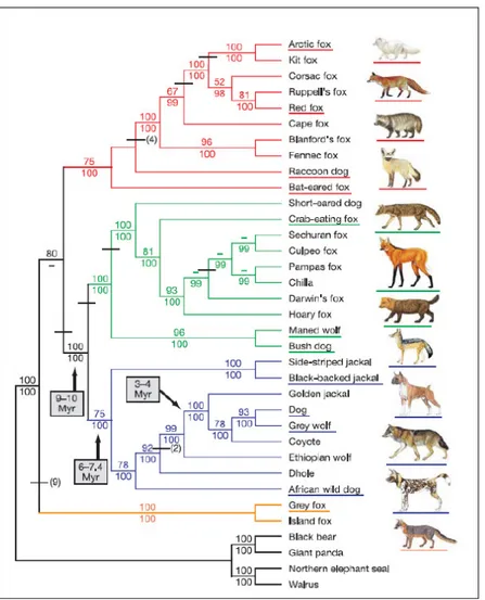
DNA sequencing (Vila et al. 1997, Leonard et al. 2002, Lindblad-Toh et al. 2005) and phylogenetic studies indicate that the gray wolf is the only ancestor of domestic dogs (Canis
Figure 2. Phylogenetic relationships among the Canidae lineages inferred from nuclear sequence data (from Lindblad-Toh et al. 2005).
Probably wolf-like canids had their origin in Africa, since the two African jackals are the most basal members of this clade. South American taxa represent another large group of canids and are clearly rooted on the two most morphologically divergent species, the maned wolf and bush dog; the red fox-like canids, which are rooted on the fennec fox and Blanford’s fox, also include the raccoon dog and the bat-eared fox. The grey fox lineage seems to be the most primitive and could suggest a North American origin of the living canids, which probably appeared about 10 million years ago.
According to these results, the first species of the genus Canis could have originated during the late Miocene, from 9 to 4.5 million years ago (Nowak 2003).
Canis sp. (Palombo et al. 2008) has been recorded in Africa at about 3.5 Mya and possibly a large-sized form could be present at Laetoli at about 3.7 Mya. Members of the genus Canis are thought to appear in Europe in the Late Pliocene or even in the Middle Pliocene. Fossil
record of the species C. lupus (Sommer and Benecke 2005) was found for the first time in Europe in assemblages of the Saalian Glacial by a very robust form, confirming the Palearctic Region to be the geographic origin of this species. The wolf is a member of the Late-Pleistocene Mammuthus-Coelodonta faunal complex and was possibly distributed in all parts of Europe during the Late-Pleistocene. Probably C. lupus ancestor originated in North America, moved to Eurasia and went back to the New World, which could have been reached several times (Leonard et al. 2002).
Wolves are highly adaptable and widely distributed in ecosystems ranging from Arctic tundra to Arabian deserts in the Old and New World (Mech 1970). Field observations, as well as population and genetic studies, indicate that wolves may disperse rapidly over long distances, either by recurrent dispersal or during waves of population expansion (Vila et al. 1999). Expanding wolf populations have rapidly recolonized suitable areas of their historical range in North America and Europe, and occasional events of long-distance dispersal have been described (Lucchini et al. 2002, Valière et al. 2003, Ciucci et al. 2009). However, permanent physiographic traits or anthropogenic habitat fragmentation may limit individual dispersal and gene flow. Wolves do not expand in agricultural landscapes, which, in contrast, are commonly used by other canids, like coyotes in North America and jackals in Eurasia (Wayne et al. 1992). Wolves were presumably widespread almost everywhere in Eurasia throughout the Holocene (Boitani 2000).
Human persecution, deforestation and the decrease of natural preys led wolf populations to decline in Europe during the last centuries (Delibes 1990). Large populations survived in the Balkans and Eastern Europe, while the species was eradicated in central Europe and Scandinavia, and only survived in fragmented populations in the Iberian and Italian peninsulas.
Studies on the control region of mitochondrial DNA (Randi et al. 2000, Vila et al. 1999) show an unexpected distribution of different haplotypes in Europe and Eastern Russia, probably due to several contraction-expansion periods and migrations, instead of a strictly geography-dependent scheme (Vila et al. 1999).
Italian wolves (Randi et al. 2000) have a mitochondrial haplotype (W14) that is unique (this fact partially supports the hypothesis made on morphological bases by Altobello in 1921 - almost one century ago – on the existence of a distinct Italian subspecies: C. lupus italicus). The causes of this process have been accurately described by (Lucchini et al. 2004). Wolves disappeared from the Alps in the 1920s and drastically declined in Italy in the two decades after World War II. By 1973 there were approximately 100 surviving individuals, isolated in
the central Apennines (Zimen and Boitani 1975). Legal protection and the expansion of natural prey populations contributed to revert the wolf decline, and a census in 1983 suggested the presence of about 220 wolves (Boitani 1984). Thereafter, wolves expanded rapidly along the Apennines ridge, recolonizing the Western Italian and French Alps in 1992 (Breitenmoser 1998, Lucchini et al. 2002, Valière et al. 2003). Ciucci and Boitani (1991) estimated an annual population increase of 7% from 1973 to 1988, leading them to argue that wolves in Italy should now number about 600 individuals, although current estimates can better suppose the existence of about 1000 wolves.
Wolves in the Apennines (Lucchini et al. 2004) could have been, at least partially, genetically isolated from any other wolf population in Europe for some thousands of years, and not just for a few decades, as suggested by information on the species’ historical distribution range. The Alpine ice caps at the last glacial maximum might have provided a geographical barrier that isolated wolves in refuge areas south of the Alps. Deglaciation and the expansion of extant ecosystems were completed only after the Younger Dryas cold spell (c. 10 000 years ago, Dawson 1996). Thus, the admixture of wolf populations expanding from different glacial refuges could have been relatively recent. Moreover, the Po River, which cuts the plain from the western Alps to the Adriatic Sea, was much more expanded during the last glaciation, because of the lower sea level and the presence of a north Adriatic land-bridge (Dawson 1996). For thousands of years in the Holocene, the Po River basin was flanked by extensive flooded alluvial plains and marshes, which were partially drained only in the last 2000 years (Sereni 1961). Admixture of Alpine and Apennines wolf populations could have been prevented also by deforestation and the concomitant eradication of wild ungulate populations, which were already widespread during the fifteenth century in northern Italy as a result of expanding sharecropping agricultural systems (Sereni 1961).
Despite the high potential rates of dispersal and gene flow (Lucchini et al. 2004) local wolf populations may not mix for long periods of time. Wolves from the Apennines are currently expanding, recolonizing parts of their historical range in the western Italian and French Alps (Lucchini et al. 2002, Marucco et al. 2009). Meanwhile, from the east, wolves with distinct mitochondrial haplotypes are moving from Slovenia towards the Italian border in the eastern Alps. It will be interesting to observe whether wolves expanding from the west (bearing Apennines haplotypes) and from the east (with Balkan haplotypes) will mix during the ongoing process of natural recolonization of the Alps.
1.3.2. Morphology and biology
Wolf weight and size can greatly vary worldwide.
In general, height varies from 0.6 to 0.95 meters at the shoulder and weight ranges from 20 to 62 kilograms. In Italy (Ciucci and Boitani 1998) the average weight of an adult male usually varies from 25 to 35 kg and it never overcomes 45 kg.
Wolves can measure from 1.3 to 2 meters from the nose to the tip of the tail, which itself accounts for approximately one quarter of the overall body length. The most remarkable dimensions can be found at high latitudes, with a maximum at about 60 degrees north
Wolves present sexual dimorphism, since females typically weight 20% less than males. They also have narrower muzzles and foreheads, smoother legs and less massive shoulders.
Wolves can cover long distances trotting at a pace of about 10 km/h, but can reach speeds approaching 65 km/h during a chase.
Wolves are digitigrades and their paws are able to tread easily on every kind of terrains. There is slight webbing between toes (Ciucci and Boitani 1998), which allows them to move on snow more easily than many preys. The front paws are larger than the hind paws, and have a fifth digit, the dewclaw, that is absent on hind paws, but never touches the ground.
The anatomical location of blood vessels – which allows a counter-current heat exchange - preserves paw pads from freezing and helps saving energy in cold climates. The same system has been maintained in ancient domestic dogs, such as Siberian husky.
Scent glands located among wolves toes leave on the ground trace of chemical markers, helping the wolf to orientate over wide territories and, in the meanwhile, to inform the other wolves of its position.
The coat of wolves consists of two layers: the first one is composed of tough guard hairs that repel water, while the second one is a dense undercoat that well insulates from external temperature. The undercoat is shed once a year in late spring or in early summer (Ciucci and Boitani 1998), increasing again from early winter months.
The coloration of the fur varies from gray to gray-brown, passing through white, red, brown, and black, sometimes according to the ecological adaptation to the habitat, as it occurs at the interface between taiga and tundra (Musiani et al. 2007).
Wolves have distinct winter and summer pelages that alternate in spring and autumn.
Italian wolves usually have black tips on tail and ears and black lines on the front legs, while abdominal parts are lighter or cream-white, as well as the face mask (Ciucci and Boitani 1998). This feature helps to emphasize certain gestures during social interactions.
Black wolves only occur in North America and Italy. Here, only few individuals have been found to have a completely black fur, which for a long time has been considered as the effect of introgression from dogs of the causative gene, β-defensin 103 (T. M. Anderson et al. 2009). However in most of the back wolves in Northern Apennines (Apollonio et al. 2004) no trace of hybridization was found, suggesting that the black coat colour can also derive from a natural combination of wolf alleles, or that the hybridization traces back thousands of years (T. M. Anderson et al. 2009). Compared to dogs, wolves show anatomical differences in the orbital angle (>53 degrees for dogs, <45 degrees for wolves), a lower frontal step, larger skull and brain capacity, as well as relatively larger paw size. Yellow eyes, longer legs, the presence of pre-caudal glands and longer teeth are other distinguishable features. Talking about dentition, the formula is I3, C1, P4, M2 / I3, C1, P4, M3 (Ciucci and Boitani 1998); the fourth upper premolars and the first lower molars are named carnassial teeth, specifically evolved for shearing flesh. The long canines (20 to 23mm), used to catch and hold the prey, can deliver a pressure up to 10,000 kPa. Teeth injuries are a serious danger for wolves, sometimes leading to starvation and death.
Hunting techniques rely on pursuit, which allows wolves to make a strong selection on physical and health conditions of preys: by choosing the most vulnerable ones, they can save energy and in the meanwhile effect a positive selection on the prey population.
The oestrus occurs once a year (whereas in dogs it occurs twice) and the mating takes place between January and April (in Italy, generally in March), according to the latitude and to the photoperiod, which regulates the hormonal production (Kreeger 2003): the higher is the latitude, the later it occurs.
The alpha pair is the only one to mate and, since a pack can usually support only one litter a year (the wolf has evolved as a K-strategy species), this dominant behaviour is beneficial in the long run and allows a continuous adaptation to the environment.
The gestation period lasts 60-64 days (Packard 2003) and adult females produce about 4-6 pups (with documented variations from 1 to 11, Mech 1974).
The pups, which weight about 0.5 kg, are born blind and completely mother-dependent. The father, often helped by others relatives or pack members, protects the home-site and carries food for the mother (Mech 1999). Pups reside for two months in the den, which is usually placed on high ground and near an open water source (Joslin 1967, Mech 1970), often at the center of the pack’s territory, to minimize the hunting effort and the pups exposition to other packs (Mech and Boitani 2003). Its features can change according to the habitat and to the
ground type and it can be adapted from other species’ den, or in a rocky cave. The pups begin to eat regurgitated food two weeks later (Packard 2003), when their milk teeth have emerged. Two months later, pups are moved to a rendezvous site (Joslin 1967), a safe place where to stay and wait for the adults during the hunts, until they will be able to join the chase (at about the 8th month of age).
The pups’ fights for eating privileges produce a secondary ranking among them and practice them to the dominance/submission rituals.
Young wolves reach sexual maturity at two or three years, when many of them (mainly the males) leave their birth packs and look for their own territories where they establish and mate. Into the wild, wolves generally live from 6 to 8 years, although in captivity they can live up to twice that age.
The mortality rates in the wild are high. Pups die for food scarcity, pathogens or for falling prey of other predators. The most significant causes of mortality for adult wolves are human hunting and poaching, car accidents and wounds inflicted while hunting prey. Rival wolf packs are often their most dangerous non-human enemies, as 14–65% of wolf deaths can be inflicted by other wolves (Huber et al. 2002).
Wolves are social animals and communication plays a great role in every moment of their life. Wolves can communicate in several ways that can be grouped in acoustic, visual and olfactory communication.
The howling is the most widely known means of communication among wolves (and can be reasonably considered one of the main sources of human fear toward wolves). The howling is a deep sound, whose fundamental frequency can range from 150 to 789 Hz, up to the 12th superior harmonic (Theberge and Falls 1967). Different wolves can howl in different ways (Ciucci and Boitani, 1998), as well as different populations can use the howling differently. Howling allows the pack members to keep in touch through forested areas or over great distances and also to meet in a specific location before a chase (Harrington and Asa 2003). Howling is important as a declaration of territory, as shown in a dominant wolf tendency to respond to a human imitation of a "rival" wolf in an area that wolves consider their own. Wolves will also howl for communal reasons, as to strengthen the social bonds. A wolf howl can be heard for several kilometers, depending on weather conditions. Wolves howl more frequently during the breeding season (Harrington and Fred 2000) and in the first half of winter.
Growls are signs of warning or threaten and are usually associated with a visual signal, whereas barks can denote a nervous mood and are much less frequently used than in dog’s communication. The rally is a high pitched noise that is often used when the wolves of a pack meet, or even to denote submission.
Visually, wolves are always communicating one to another through body language, which comprehends body carriage, tail and ears postures and facial expressions, usually enhanced by the light mask around the muzzle. A large combination of these coded signals can share feelings and underline hierarchical relationships, as dominance, submission, anger, fear, aggression or defensive attitude, suspicion or tension, but also relaxation, happiness or playfulness.
Another crucial form of communication in wolves is the olfactory-based one (which is probably the most difficult for us to understand and even imagine), since smell is the most developed sense in wolves, with about 1000 genes dedicated to this function (Tacher et al. 2005).
Scent glands are present all over the body, especially at the base of the tail or among toes (Harrington and Asa 2003). Pheromones secreted by these glands can identify each single wolf, its health conditions, and its social and reproductive status. Alpha wolves scent-mark frequently, with both faeces and urine. Male and female alpha wolves usually urine-mark objects with a raised-leg stance (RLP) in order to enforce rank and territory, whereas other pack members usually squat. Defecation markers are particularly useful for spatial navigation and are often deposed along frequently used paths or in important crossroads (Barja et al. 2004), keeping the pack from traversing the same terrain too often and allowing each wolf to know of the whereabouts of its pack members. Ground-scratching is the main way to depose the scent of the inter-toes glands. Above all, scent marking is used to inform other wolves and packs that a certain territory is occupied.
Wolves live in packs (Mech 1970), hierarchically ruled social units that can comprehend from two to ten individuals (even more at high latitudes). Living in pack allows wolves to reach a good hunting and reproductive success. The ranking within the pack can be defined as a linear dominance hierarchy and the two individuals that lead the pack (one for each sex) are also called alpha male and alpha female. They are usually monogamous until the death of one of them and they are the only individuals that can reproduce in a pack, although multiple litters have been documented (Vonholdt et al. 2008). The members of the alpha pair have the greatest control over food resources, but also keep the pack cohesive and functional (Mech 1970), leading it in the everyday decisions and in territory defence, especially by the male
(Packard 2003). The ranking is decided on the base of ritual, agonistic behaviors and it can change from year to year, in particular before the reproductive period.
All the wolves of the pack assist in raising the pups. Some mature individuals can choose not to disperse and stay in their original pack helping rear pups.
As we said, usually wolves packs (Packard 2003) are considered to be organized as a linear hierarchy, but the concept of family may better describe the relationships and the dynamics among its members. A pack, indeed, is always composed by the mating pair, their pups (if any) of the year and of the prior years, plus some external individuals (the adoptees) that can come by dispersal events from other packs (Mech and Boitani 2003).
Dispersal reduces the resource exploitation in a single territory, prevents inbreeding and promotes natural selection and cross-breeding.
The size of the pack may change over time according to several factors, including habitat, food supply and even personalities of individual wolves within a pack. New packs are formed when a wolf leaves its birth pack, finds a mate, and claims a territory (Rothman and Mech 1979).
Territory size, as well as the number of members, can greatly vary (20 km2-4335 km2) and is
negatively correlated with the available prey biomass, which is related to the habitat and also to the latitude. In Italy, the territory size can range from 20 to 300km2 (Apollonio et al. 2004; Ciucci and Boitani 1998).
Although the main prey is represented by large herbivores (wild boar, roe deer, red deer, moose, mouflon, even bison), which are chased with the cooperation of the whole pack and accurate attack techniques (e.g. at first to the legs, then to the neck, with precise bites that produce an hypo-oxygenation shock), they can also hunt rodents and other small animals. In northern America the bison is the largest prey that wolves use to hunt, while in northern Europe it is the moose. Hunting success seems to be related to the pack size and to the presence and age -therefore the experience- of an adult male (Sand et al. 2006). In Italy, also garbage has represented an important food source during the years of maximal reduction. As keystone predators, wolves have a great impact on the trophic network, but at the same time they are also vulnerable to prey fluctuations.
Predations on livestock are quite common in rural areas, and surplus killing has been documented, but not completely explained.
1.3.3. Threats and legal status
As we saw, wolves have been progressively eradicated throughout Western Europe and in the Alps in the 18th and 19th centuries (Breitenmoser 1998), surviving in fragmented populations in Iberian peninsula and Italy (Boitani 2003). Wolves in Italy were confined south of the Po River since the turn of the last century, continuing to decline until the 1970s, when approximately 100 individuals ranged in two fragmented areas in central-southern Apennines (Zimen and Boitani 1975). The Italian wolf population suffered severe persecution until 1971, when wolf hunting was stopped and poison baits banned. This change of attitude was completed in 1976 when the species was given a fully protected status. This process was stimulated by WWF International that funded a long-term project called “San Francesco”, including a public educational campaign, scientific works and management solutions to protect wolves. Due to the more effective legal protection and, above all, substantial changes in the ecology of mountain areas (e.g. decrease of human density and increase of wild ungulates), this declining demographic trend quickly reversed in the 1980s, when wolves started to expand in Italy and in other European countries (Breitenmoser 1998; Boitani 2003). In Italy wolves crossed the northern Apennines and recolonized the south-western Alps, where genetic identification confirmed their presence in France and in Switzerland (Fabbri et al. 2007, Lucchini et al. 2002, Valière et al. 2003), and reappeared again in the central Italian Alps in 2000. Few years ago the Italian wolf population was guessed to number more than 600 individuals (Boitani 2003), being now probably closer to 1000 individuals.
The wolf is considered a species of Least Concern (2007 IUCN Red List of Threatened Species) by the World Conservation Union, but it is currently legally protected in Italy through international law, European law and Italian law.
For every detail, we refer to the National Action Plan for Conservation of Wolf (Genovesi 2002), that collects the best knowledge and practices on the conservation of wolves in Italy in order to coordinate the actions for its management.
The wolf is protected under international law, primarily under the Bern Convention on Conservation of Wildlife and Natural Habitats (1979), in appendix II (Strictly Protected Species). The convention forbids its catching, killing, possession and trade. However, many countries in Eastern and Northern Europe refused to fully protect the wolf, and Spain has recently authorized its hunting.
Also the Convention on International Trade of Endangered Species of Fauna and Flora (CITES, Washington 1973) strictly protects several wolf populations (the ones from Bhutan, India, Nepal and Pakistan) in Appendix I (species threatened with extinction which are or