2018
Publication Year
2020-12-29T11:42:15Z
Acceptance in OA@INAF
Athena X-IFU synthetic observations of galaxy clusters to probe the chemical
enrichment of the Universe
Title
Cucchetti, E.; Pointecouteau, E.; Peille, P.; Clerc, N.; RASIA, ELENA; et al.
Authors
10.1051/0004-6361/201833927
DOI
http://hdl.handle.net/20.500.12386/29277
Handle
ASTRONOMY & ASTROPHYSICS
Journal
620
Number
https://doi.org/10.1051/0004-6361/201833927 c ESO 2018
Astronomy
&
Astrophysics
Athena X-IFU synthetic observations of galaxy clusters to probe
the chemical enrichment of the Universe
E. Cucchetti
1, E. Pointecouteau
1, P. Peille
2, N. Clerc
1, E. Rasia
3, V. Bi
ffi
3,4, S. Borgani
3,4,5, L. Tornatore
3,
K. Dolag
6,7, M. Roncarelli
8,9, M. Gaspari
11,?, S. Ettori
9,10, E. Bulbul
12, T. Dauser
13, J. Wilms
13,
F. Pajot
1, and D. Barret
1 1 IRAP, Université de Toulouse, CNRS, CNES, UPS, Toulouse, Francee-mail: [email protected]
2 CNES, 18 Avenue Edouard Belin, 31400 Toulouse, France
3 INAF, Osservatorio Astronomico di Trieste, Via Tiepolo 11, 34131 Trieste, Italy
4 Dipartimento di Fisica dell’Università di Trieste, Sezione di Astronomia, Via Tiepolo 11, 34131 Trieste, Italy 5 INFN – National Institute for Nuclear Physics, Via Valerio 2, 34127 Trieste, Italy
6 University Observatory Munich, Scheinerstr. 1, 81679 Munich, Germany
7 Max Plank Institut für Astrophysik, Karl-Schwarzschield Strasse 1, 85748 Garching bei Munchen, Germany 8 Dipartimento di Fisica e Astronomia, Università di Bologna, Via Gobetti 93, 40127 Bologna, Italy
9 INAF, Osservatorio di Astrofisica e Scienza dello Spazio, Via Pietro Gobetti 93/3, 40129 Bologna, Italy 10 INFN, Sezione di Bologna, Viale Berti Pichat 6/2, 40127 Bologna, Italy
11 Department of Astrophysical Sciences, Princeton University, Princeton, NJ 08544, USA 12 Harvard-Smithsonian Center for Astrophysics, 60 Garden Street, Cambridge, MA 02138, USA
13 Dr. Karl Remeis-Observatory and Erlangen Centre for Astroparticle Physics, Sternwartstr. 7, 96049 Bamberg, Germany
Received 23 July 2018/ Accepted 24 September 2018
ABSTRACT
Answers to the metal production of the Universe can be found in galaxy clusters, notably within their intra-cluster medium (ICM). The X-ray Integral Field Unit (X-IFU) on board the next-generation European X-ray observatory Athena (2030s) will provide the nec-essary leap forward in spatially-resolved spectroscopy required to disentangle the intricate mechanisms responsible for this chemical enrichment. In this paper, we investigate the future capabilities of the X-IFU in probing the hot gas within galaxy clusters. From a test sample of four clusters extracted from cosmological hydrodynamical simulations, we present comprehensive synthetic observations of these clusters at different redshifts (up to z ≤ 2) and within the scaled radius R500performed using the instrument simulator SIXTE. Through 100 ks exposures, we demonstrate that the X-IFU will provide spatially resolved mapping of the ICM physical properties with little to no biases (/5%) and well within statistical uncertainties. The detailed study of abundance profiles and abundance ratios within R500also highlights the power of the X-IFU in providing constraints on the various enrichment models. From synthetic obser-vations out to z= 2, we have also quantified its ability to track the chemical elements across cosmic time with excellent accuracy, and thereby to investigate the evolution of metal production mechanisms as well as the link to the stellar initial mass-function. Our study demonstrates the unprecedented capabilities of the X-IFU of unveiling the properties of the ICM but also stresses the data analysis challenges faced by future high-resolution X-ray missions such as Athena.
Key words. galaxies: clusters: intracluster medium – galaxies: abundances – galaxies: fundamental parameters – techniques: imaging spectroscopy – methods: numerical – X-rays: galaxies: clusters
1. Introduction
Metals and other heavy elements in the intra-cluster medium (ICM) represent a fossil record of the chemical evolution of the Universe. Trapped in the dark matter (DM) potential of galaxy clusters (White et al. 1993), they remain unaltered within the optically-thin, collisionless thermal plasma. Elements originate within stars or through supernovæ (SN), before being spread by stellar winds or by the SN explosions. Hence, the chemical enrichment of a given cluster relates to the integrated star forma-tion history of the cluster, as well as to the overall stellar initial mass function (IMF). The abundances and spatial distribution of metals in the ICM can also be connected to its dynamical history and to the mechanical action of active galactic nuclei (AGNs) outflows or jets (e.g.Gaspari et al. 2011).
? Einsteinand Spitzer Fellow.
Most of the low-mass elements (C, O, Mg, Si, and S) are pro-duced by end-of-life massive stars (≥10 M ) undergoing core-collapse supernovæ (SNcc; seeNomoto et al. 2013, for a review). The evolution of SNcc-related enrichment through time is dic-tated by the initial mass and metallicity of the progenitor star. High-mass elements, from Si-like elements (Al, Si, S, Ca, and Ar) to Fe and Ni, are on the other hand the result of thermonu-clear reactions occurring during the explosion of white dwarfs (type Ia supernovæ – SNIa; Hillebrandt et al. 2013). Although the mechanisms of these explosions – either via accretion of a companion star onto the white dwarf (Whelan & Iben 1973) or via mergers of binary systems (Webbink 1984) – is still poorly understood (seeMaoz et al. 2014), the timescale of these events, related to longer-living low-mass stars, suggests a later enrichment across cosmic time. Traces of other elements (C, N, Ne, and Na) can also be produced when low- and
Open Access article,published by EDP Sciences, under the terms of the Creative Commons Attribution License (http://creativecommons.org/licenses/by/4.0),
intermediate-mass stars (typically ≤6 M ) enter their asymp-totic giant branch (AGB) phase (Iben & Renzini 1983). The individual study of these phenomena based on detailed obser-vations of nearby SN is difficult as they are very rare. Rather than a direct study on stellar populations, the detailed spec-troscopic study of the ICM is an interesting alternative probe to test metal production models up to the early periods of the Universe.
Beyond the first steps in high-resolution X-ray spec-troscopy (Canizares et al. 1979, 1982) and despite the lack of spatial resolution (Peterson & Fabian 2006), the advent of high-resolution grating instruments such as XMM-Newton/RGS (den Herder et al. 2001) and Chandra/HETG (Canizares et al. 2005) drastically changed our view of the ICM enrichment, by giving access for the very first time to a large number of atomic lines (de Plaa et al. 2007; de Plaa 2013; Molendi et al. 2016;
Werner et al. 2007). Clusters have, therefore, become excellent laboratories in which to test plasma physics and the chemical enrichment models up to the present epoch (see Werner et al. 2008, for a review). Despite limited spectral resolutions, instru-ments based on charged coupled devices (CCDs) have also been pushed to the maximum of their abilities to benefit of their spa-tial resolution in investigating the spaspa-tial distribution of chemical elements in the ICM (de Grandi & Molendi 2009;Mernier et al. 2016a,b,2017).
The perspective of micro-calorimeter-based imaging spec-trometers, such as the soft X-ray spectrometer (SXS) on board Hitomi (Takahashi et al. 2016), has opened new pos-sibilities in studying the ICM: from the spatial scales of the enrichment (sources of production, processes of mixing and dispersion) to the kinematics of the hot gas (turbulence, shocks Hitomi Collaboration 2016,2018a,b,c), which comple-ment the indirect estimates via surface brightness and warm gas tracers (e.g.Churazov et al. 2012;Gaspari & Churazov 2013;
Hofmann et al. 2016; Gaspari et al. 2018). Unfortunately, the short lifetime of the SXS gave only a glimpse of its potential. These renewed capabilities in galaxy-cluster observation now rely on future missions, such as the X-ray Recovery Imaging and Spec-troscopy Mission (XRISM;Ishisaki et al. 2018) or the Advanced Telescope for High-ENergy Astrophysics (Athena;Nandra et al. 2013). Namely, the X-ray Integral Field Unit (X-IFU) on board the future European X-ray observatory (Barret et al. 2016;Pajot et al. 2018), will provide narrow-field observations (50 in equivalent field-of-view diameter) over the 0.2–12 keV bandpass, with a required 500spatial resolution and an unprecedented spectral res-olution of 2.5 eV (required up to 7 keV).
Investigating the chemical enrichment of the Universe is one of Athena’s prime science objectives (Ettori et al. 2013;
Pointecouteau et al. 2013) which drives top-level performances of the telescope . In addition to the spectral resolution of the X-IFU, which will allow to resolve faint atomic lines of less abundant elements, this science objective drives the need for a high effective area of the telescope along with a well-calibrated low energy band, required to accurately resolve lines of light elements such as C (≥0.2 keV). Number of breakthroughs on the study of chemical species and their evolution should in fact come from measurement in the low-energy band, where the effective area is the highest. The fine spectroscopic capa-bilities of the X-IFU in this energy band will probe the pro-duction and circulation of metals within galaxy clusters across cosmic time, up to a redshift of z ≤ 2 and a distance of R5001 from the cluster’s centre. By accurately measuring the
1 R
500is the radius including a density contrast of 500 times the critical density of the Universe, ρc= 3H(z)2/8πG, at the given redshift z.
abundances of the most common elements (e.g. O, Si, S, and Fe), the X-IFU will be capable of constraining the number of time-integrated SNIa and SNcc products. For the first time, the spatially-resolved measurements of less abundant elements (e.g. C, Al, S, and Ca) as well as rare elements (e.g. Mn, Cr, and Ti) will provide insights on the initial metallicity of the SNIa progenitors, and therefore on their formation mechanisms. The science of the chemical enrichment is a driver of the perfor-mance of the instrument, which needs to be assessed before launch.
In this paper, we investigate the feasibility of recovering the physical parameters of the ICM through X-IFU observations. Careful attention is given to the different enrichment mech-anisms and their evolution over time. We used a sample of four simulated galaxy clusters with different masses studied at different redshifts, obtained via hydrodynamical cosmological simulations (Rasia et al. 2015;Biffi et al. 2017). These objects are passed as input to a dedicated end-to-end (E2E) simula-tion pipeline of the X-IFU instrument, based on the simulator SIXTE (Wilms et al. 2014). In Sect.2, we present the proper-ties of the sample of simulated clusters. This is followed by a detailed description of our simulation pipeline (Sect.3). The data analysis, post-processing procedures and results validation are in turn described (Sect.4). The outputs of our synthetic obser-vations obtained through the pipeline for the four local clusters are then used (Sect.5) to infer the main properties of the sam-ple and study its enrichment. This investigation is also extended to higher redshift values (Sect.6) to look into the X-IFU abil-ities to capture the evolution of abundances through cosmic time. Finally, results and outcomes of our study are discussed (Sect.7).
2. Generation of the cluster sample
The sample of four clusters of galaxies analysed in this study is taken from Biffi et al.(2018) and includes two massive and two smaller systems, to bracket a broad mass range across the considered redshift values (Table 1). In both mass bins, we choose a cool-core (CC) and a non-cool-core cluster (NCC), defined based on their pseudo-entropy profiles as described in
Leccardi et al. (2010). This small sample gives a view of part of the expected cluster population planned to be investigated by the X-IFU. The objects are part of a larger set of 29 Lagrangian regions extracted from a parent cosmological DM-only simu-lation and re-simulated at higher resolution including baryons (seeBonafede et al. 2011). The parent cosmological volume is 1 h−1Gpc per side and adopts a Λ-CDM cosmological model with ΩM = 0.24, Ωb = 0.04, H0 = 72 km s−1Mpc−1 (i.e. H0 = h × H100, where h= 0.72 and H100= 100 km s−1Mpc−1), σ8 = 0.8 and ns = 0.96, consistent with WMAP-7 constraints given inKomatsu et al.(2011).
The magnification simulations were performed with a ver-sion of the tree-PM smoothed particle hydrodynamics (SPH) code GADGET-3 (Springel 2005), including an improved hydro-dynamical scheme (Beck et al. 2016) and a variety of physi-cal processes describing the evolution of the baryonic compo-nent (seeRasia et al. 2015, for more details). Briefly, these com-prise metallicity-dependent radiative cooling (Wiersma et al. 2009), star formation and stellar feedback (thermal super-nova feedback and galactic winds, see Springel & Hernquist 2003), cold and hot gas accretion onto super-massive black holes powering AGN thermal feedback (Steinborn et al. 2015; modelling the action of cold accretion Gaspari & Sdowski 2017), and metal enrichment (Tornatore et al. 2004, 2007)
Table 1. Properties of the simulated clusters at different redshift values in their evolution. Name C1 C2 C3 C4 Type CC NCC CC NCC z= 0.105 R500(kpc h−1) 723 799 1027 1009 M500(M h−1) 2.39 × 10¹⁴ 3.22 × 10¹⁴ 6.86 × 10¹⁴ 6.51 × 10¹⁴ T500(keV) 3.22 4.20 6.47 6.36 z= 0.5 R500(kpc h−1) 552 676 694 715 M500(M h−1) 1.55 × 10¹⁴ 2.84 × 10¹⁴ 3.08 × 10¹⁴ 3.38 × 10¹⁴ T500(keV) 2.88 4.06 4.58 4.84 z= 1.0 R500(kpc h−1) 389 396 446 570 M500(M h−1) 0.92 × 10¹⁴ 0.97 × 10¹⁴ 1.38 × 10¹⁴ 2.89 × 10¹⁴ T500(keV) 2.41 2.47 3.12 4.41 z= 1.48 R500(kpc h−1) 269 289 345 351 M500(M h−1) 0.50 × 10¹⁴ 0.62 × 10¹⁴ 1.07 × 10¹⁴ 1.12 × 10¹⁴ T500(keV) 1.76 2.10 3.07 3.08 z= 2.0 R500(kpc h−1) 174 181 220 215 M500(M h−1) 0.23 × 10¹⁴ 0.25 × 10¹⁴ 0.45 × 10¹⁴ 0.42 × 10¹⁴ T500(keV) 1.19 1.55 2.24 1.86
from SNIa, SNcc, and AGB stars. Specifically, we assumed the IMF by Chabrier (2003), the mass-dependent life-times by Padovani & Matteucci (1993) and stellar yields by
Thielemann et al. (2003) for SNIa, Woosley & Weaver (1995) andRomano et al.(2010) for SNcc, andKarakas(2010) for AGB stars.
In our model of chemical enrichment, we follow the pro-duction and evolution of 15 chemical species: H, He, C, Ca, O, N, Ne, Mg, S, Si, Fe, Na, Al, Ar, and Ni. These elements are the individual species traced in the simulations. Although these do not cover the full spectrum of interest (lacking e.g. Mn or Cr, which are important tracers of the enrichment as recently shown in Hitomi Collaboration 2017; Simionescu et al. 2018), the variety of abundances provides a good starting point for a meaningful study on the ICM and the demonstration of the X-IFU capabilities in this view. For every gas particle in the simulation, we traced the chemical composition and the frac-tion of each metal that is produced by the three enrichment sources (i.e. SNIa, SNcc, AGB; see Biffi et al. 2017,2018, for further detail). Each object is analysed at different redshifts, z= 0.105, 0.5, 1, 1.48, and 2, to assess the enrichment through time. Table 1 provides the characteristic radius, R500, along with the mass, M500, and the mass-weighted temperature, T500, of the associated sphere of radius R500 for the entire cluster sample.
For each SPH particle, the output quantities provided by GADGET-3 are used as input for our simulation. These include the position of the particle, x, its 3D velocity in the observer’s frame, v, its mass density, ρ, its mass, m, its temperature, T , and the individual masses of the 15 individual chemical species X, µX, tracked in the simulations. The gas density n of each SPH particle is obtained by dividing ρ by m. The mass of each ele-ment of atomic mass number AXis converted into abundances ZX, expressed in solar metallicity units assuming the solar frac-tions Z ,XfromAnders & Grevesse(1989). Abundances can be therefore written as ZX= 1 Z ,X × µX µH× AX , (1)
with µHthe hydrogen mass of the particle.
3. End-to-end simulations
In this section, we describe in detail the set-up of the pipeline used for the synthetic X-IFU observations, as well as the physi-cal assumptions made in the simulations.
3.1. Synthetic X-IFU observations
Simulations of the cluster data set are carried out using the X-IFU end-to-end (E2E) simulator SIXTE2(Wilms et al. 2014),
which creates realistic X-IFU observations. SIXTE uses as an input a specific SIMPUT file (Schmid et al. 2013) containing either all the emission spectra of the particles or directly a photon list, with the time, coordinates on the sky and energy of the emitted photons. This second approach is preferred for our simulations, as it exerts a lower computational demand, induced in the former by the unparallelised random generation of photons currently implemented in SIXTE (an example of the first approach is given inRoncarelli et al. 2018). SIXTE outputs are generated not only considering the instrumental spatial and spectral responses, but also incorporate other features from the detectors such as their geometry, vignetting and internal particle background.
3.1.1. Photon list generation
Each simulated cluster comes as a list of SPH particles, which may emit X-ray photons. To generate the photon list used in the E2E simulation, the particle emission is modelled by a collisional diffuse thermal plasma using the APEC code (Smith et al. 2001). More specifically, the vvapec model on XSPEC (Arnaud 1996) is adopted, as it can be parametrised according to the particles physical properties listed above, notably the individual abundances of each element. The cor-responding atomic database used for the emission model is derived from ATOMDB v3.0.9. For the galactic absorption, the wabs model (Morrison & McCammon 1983) is preferred for computational speed, although more accurate absorption mod-els do exist (e.g. TBabs,Wilms et al. 2000). For all four clusters 2 http://www.sternwarte.uni-erlangen.de/research/
we fixed the column density to nH = 0.03 × 1022cm−3, which is a representative value for the latitudes at which most clus-ters shall be observed with X-IFU (Kalberla et al. 2005). Abun-dances are set to solar as per Anders & Grevesse (1989) and atomic cross-sections are taken as perVerner et al.(1996). The overall flux, F (in counts s−1cm−2), of each particle is computed using the vvapec normalisation N (emission-measure-weighted by the distance in units of cm−5):
N = 10
−14 4π[DA(1+ z)]2
Z
nenpdV, (2)
where DAis the angular distance of the particle computed from its redshift z (derived from the speed of the particle and the cluster mean redshift), and V the particle volume. We consid-ered a full ionisation of the intra-cluster gas with ne = 1.2np (neand np being the densities of electrons and protons, respec-tively). These emission spectra are considered as probability density distribution function and normalised accordingly over the instrumental energy bandpass (i.e. 0.2–12 keV). For a fixed exposure time∆t, photons are drawn from the afferent probabil-ity distribution following a Poisson statistic of parameter F∆tA, where A is the total mirror area (taken at 1.4 m2at 1 keV, energy dependence of the effective area is included later on in SIXTE via the ancillary response function – ARF as explained below). Each newly created photon is added to the photon list with the sky coordinates of its parent particle (right ascension and declination).
The output product of this stage is a “complete” photon list (with their true energy and position) at the entrance of the tele-scope. This list is computed once for each cluster, and contains a large number of simulated photons (≥1 Ms). It is then sam-pled randomly by SIXTE to achieve smaller lists for more typi-cal exposure times (e.g. 100 ks).
3.1.2. Observational setup
For each simulation, we consider an exposure time∆t = 100 ks over the entire X-IFU field-of-view. The complete photon list is used as input for the xifupipeline function of SIXTE, which samples the photon list accounting for the energy-dependence of the effective area to create the event list seen by the X-IFU detector over ∆t. The pipeline accounts for the most up-to-date responses of the current baseline of the telescope (i.e. 15-row mirror modules corresponding to a mirror e ffec-tive area of 1.4 m2at 1 keV3) and for a hexagonal detector array
of 3832 micro-calorimeter pixels, more specifically Large Pixel Array 2 (LPA2) pixel configuration, developed for the X-IFU and described in Smith et al. (2016). Pile-up, telescope point spread function, vignetting and detector geometry effects are also included as function of the pixels corresponding off-axis angles. Finally, we verified that given the low count rates of our clusters (≤1 cts s−1pix−1), pile-up and cross-talk over the obser-vation can be neglected (seeden Hartog et al. 2018;Peille et al. 2018).
For each cluster, we simulated enough pointings to map the cluster spatially up to at least R500 (as required in the current science objectives for the X-IFU). This translates, for local clus-ters, into at least seven pointings. The corresponding event lists are then merged during post-processing to obtain a single event file.
3 RMF: athena_xifu_rmf_v20171107.rmf| ARF: athena_xifu_ 15row_onaxis_pitch249um_v20171107.arf
Table 2. Parametrisation of the galactic foreground model used in the simulation with a apec + phabs*apec model.
Model Parameter Unit Value
apec T keV 0.099
apec Z 1
apec z 0
apec Norm cts s−1amin−2 1.7 × 10⁻⁶
phabs nH 1022cm−3 0.018
apec T keV 0.225
apec Z 1
apec z 0
apec Norm cts s−1amin−2 7.3 × 10⁻⁷
3.2. Foreground and background components
In addition, we accounted for the contribution of different fore-ground and backfore-ground sources to ensure more representative observations.
3.2.1. Astrophysical foreground
The foreground emission is caused by the X-ray emission of the local bubble in which the solar system is embedded and by the Milky Way hot gaseous content. This component can be modelled by the sum of a non-absorbed and absorbed thermal plasma emission as specified in McCammon et al. (2002) and parametrised as per (Lotti et al. 2014, see Table2). An additional normalisation constant over the entire model is used for versa-tility purposes, resulting in a total foreground model reading as constant*(apec + phabs*apec) in XSPEC. This component is folded into SIXTE using a SIMPUT file.
3.2.2. Cosmic X-ray Background
The cosmic X-ray background (CXB) component is due to the contributions of AGNs, star forming galaxies and active stars along the line-of-sight (Lehmer et al. 2012). A fraction of these sources will be resolved by the instrument as a func-tion of its spatial resolufunc-tion, and will be excised from the observations. Given the requirement on the spatial resolution for Athena/X-IFU (500), 80% of the total flux of these point sources in terms of the integral of their log(N)/log(S) distribu-tion should be resolved by the instrument (Moretti et al. 2003). For 100 ks exposure times, this translates into limiting fluxes of ∼3 × 10⁻¹⁶ergs s−1cm−2 for the X-IFU. As the number of star forming sources is at least an order of magnitude lower at this flux, we only considered the AGN contribution in this study. The unresolved fraction of these point sources results in a diffuse background component, which we classically fit-ted using an absorbed power-law model during post-processing (McCammon et al. 2002).
We did not include AGN point sources in the inputs derived from the hydrodynamical simulations. Instead, to generate real-istic CXB data, we drew a list of AGN sources with asso-ciated X-ray spectra by sampling the luminosity function of
Hasinger et al.(2005) in the luminosity-redshift space, given the boundary conditions LX ≥ 1042erg s−1 unabsorbed 0.5–2 keV rest-frame luminosity, 0 < z < 5 and the size of the cosmo-logical volume encompassed within a field-of-view. Each source is associated with a spectral energy distribution following tem-plates described inGilli et al.(2007), according to a distribution
of power-law indexes and intrinsic absorption column densi-ties related to various levels of obscuration, as described in
Gilli et al. (1999,2007). Spatial distributions are fully random in the sky plane (no clustering). Further details about the proce-dure can be found inClerc et al.(2018). This component is also included in the simulations using a SIMPUT file.
3.2.3. Instrumental background
The instrumental particle background is caused by interac-tions of high-energy cosmic rays and protons with the instru-ment structure, which create secondary particles in the soft X-ray band. Both primary and secondary particles can hit the detectors and be recorded as regular events. The X-IFU design includes an onboard cryogenic anti-coincidence detec-tor (Macculi et al. 2016), which will ensure the required level of 5 × 10⁻³counts s−1keV−1cm−2over the 2–10 keV energy band (Lotti et al. 2017). The generation of this component is directly implemented within SIXTE.
For each of these three background components, we asso-ciate a flag on the photons in the event file. Thus, these specific events can be respectively masked to study background effects on the observations (notably of the internal particle background) or selected exclusively to generate background maps. Through-out this study, we assume that these background components have no systematic uncertainty. Systematic effects of the back-ground knowledge on the observations are discussed Sect.7and are considered in more ample detail elsewhere (Cucchetti et al. 2018).
4. Data processing
In this section we describe the post-processing approach used in our simulations and its validation.
4.1. Source contamination
From the event list output of SIXTE, a first selection is made on the grading of the events, which is conditioned by the frequency of detection in a given pixel and defines the spectral resolution of the event. In practice, the grading procedure will occur in-flight using the onboard event processor depending on the time sepa-ration between events in the same pixel (Peille et al. 2018), sim-ilarly to the strategy implemented on the SXS (Seta et al. 2012). In this case, grading occurs automatically within the simulator and is available in the event list. Only high-resolution events corresponding to∆E = 2.5 eV, the required spectral resolution for X-IFU, were used. As the count rates of the clusters are low over the entire field-of-view (≤1 count s−1pix−1), almost all events (throughput ≥99%) are high-resolution photons. Events with lower grading values are discarded in the rest of the study.
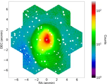
Using the selected events, we reconstructed raw brightness maps in counts as presented in Fig. 1. Beside the ICM, emis-sion from other sources either present in the hydrodynamical simulations (i.e. strongly-emitting particles or clumps) or in the CXB can be observed. For the CXB, following the assump-tion byMoretti et al.(2003), we start by selecting the brightest simulated sources (with fluxes above ∼3 × 10⁻¹⁶ergs s−1cm2, see Sect. 3.2.2). After simulating CXB-only pointings to find their coordinates on the detector, these sources were excised automatically from the brightness maps by finding all the cor-responding pixels above a 2σ threshold in counts with respect to the average count in neighbouring pixels in the event list.
This way, the diffuse emission of the cluster is accounted for when masking a pixel. The average cut-off flux of the sources will be higher than ∼3 × 10⁻¹⁶over the full map. The lower the emission (e.g. in the outskirts), the closer the limiting flux of the excised point-sources will be to the threshold flux. Although this process would not be possible for real event files, we adopted this strategy to avoid potential biases related to spe-cific point-source detection algorithms. Once these sources are removed, a final visual inspection was performed to remove any residual unexcised AGNs as well as any remaining visible point-like source which may be related to the hydrodynamical simulations.
4.2. Spatial binning
For the considered exposure time of 100 ks, single pixels do not always capture enough photons to allow the measurement of chemical abundances. We therefore grouped them into regions to increase the signal-to-noise ratio (S/N) adequately.
Two methods were considered to spatially bin the pixels: the contbin tool developed bySanders(2006) and an adapted 2D Voronoï tessellation method byCappellari & Copin(2003). Both methods were tested and a comparison showed no visi-ble difference in accuracy of the pipeline (see also AppendixA
or Sanders 2006 for a more detailed comparison). Unlike the Voronoï tessellation, contour binning offers better results in describing the radial-like shape of the cluster emission, and was therefore retained for this study. The contbin binning scheme can be directly applied to our cluster count maps to compute regions of equal S/N. The real exposure map (con-stant here) and the spatial mask of excised sources are also used as inputs of the algorithm. In addition, we chose to fix the aspect-ratio of the binning regions (so-called constrain filling-factor) to two, to avoid long radial filamentary regions, which could artificially mix spatially-uncorrelated structures (espe-cially in low count rates areas such as the outskirts of the cluster).
The binning procedure operates on the count maps, which are dominated by the ICM bremsstrahlung emission, that is, the continuum of the spectral energy distribution. We further optimised our pixel binning in view of our scientific objective of measuring chemical abundances and to account for smaller local surface brightness variations atop the bulk of the clus-ter emission due to for example, clumps or bubbles. To do so, we first divided the surface brightness map into annuli centred on the brightest part of the cluster and containing roughly the same number of counts (∼300 000). For each of these annu-lar regions, the total spectrum of the annulus is fitted over the entire bandpass (0.2–12 keV) with a continuum-only vvapec model (metal abundances set to zero) to estimate the number of counts in the continuum for a given annulus Ccontinuum only. Although slightly overestimating counts (due to the presence of lines), this simple approach converges quickly. When abun-dances are left free then set to zero after the fit, strong lines are sometimes spaced by values of the order of the energy res-olution of the instrument (due to strong bulk motion or clump-ing within the cluster), causclump-ing fits to converge on local min-ima or not at all. Even after convergence, differences from the previous method do not exceed ≤3%. The total number of counts on a pixel i (Ci) in the annulus is then re-scaled as follows: ¯ Ci= 1 − Ccontinuum only Ctotal annulus ! Ci (3)
Fig. 1.Maps in number of counts per X-IFU pixel (249 µm pitch) for our clusters 1 to 4 (see Table1) at redshift z= 0.1. Each mosaic is made of 7 X-IFU pointings of 100 ks each.
Fig. 2.Example of a continuum subtracted count map for cluster C2 used for spatial binning. Each of the ∼27 000 pixels was re-scaled as explained in Sect.4.2to enhance density contrasts in the cluster.
The resulting template image for cluster C2 can be seen Fig.2. This approach allows to define regions over a continuum sub-tracted image, enhancing the brightness fluctuations with respect to the azimuthal continuum model due to chemical elements emis-sion and other local density contrasts. This template image is used exclusively for spatial binning. Accounting for its statistics, we requested a S/N level of 30 (900 counts in regions) to contbin. The resulting spatial regions are used over the full count maps to compute the corresponding spectra. Given a count ratio of ∼100 between the template map and the full surface brightness map, we ensure that each spectrum has a high statistical significance, that is, S /N ∼ 300. This represents a total of at least 90 000 counts per region, in other words three counts in each instrumental channel, allowing high significance regions for the fits.
This binning approach has been used throughout this paper when statistics allows it, that is, in the case of local clusters (z ≤ 0.5). For high-redshift clusters, count rates are often insuf-ficient to ensure statistically independent regions with a high-enough S/N. In this case, we followed the formulation of the Athenascience objectives on chemical evolution of the Universe (specified in the introduction) and considered two radial annular regions, over 0–0.3 R500and over 0.3–1 R500.
4.3. Accounting for vignetting effects
Despite the narrow field-of-view of the X-IFU, the Athena tele-scope will introduce a slight vignetting effect in the observations (between 4 and 8% of the counts over the energy bandpass). Vignetting is simulated within SIXTE using tabulated values derived from ray-tracing simulations of the mirror assemblies (Willingale et al. 2014) and needs to be accounted for before attempting a spectral fit. To do so, for each binned region, the baseline X-IFU effective area of every single pixel is multiplied over the energy bandpass by the same vignetting function imple-mented in SIXTE accounting for the off-axis position of the pixel. The specific response function of the entire region is then obtained by averaging, in each energy channel, the response of each of pixels weighted by their respective number of counts. 4.4. Temperature and metal maps
The resulting unbinned spectra were fitted within XSPEC, using a log-normal likelihood minimisation (i.e. C-statistics adapted fromCash 1979), which is well adapted for Poissonian data sets (i.e. channels with low number of counts). An absorbed single-temperature thermal plasma model (i.e. wabs*vvapec) was fit-ted to the spectrum accumulafit-ted in each region. The column density nHis fixed to its input value, while temperature, abun-dances of metals traced in the input numerical simulations, (see Sect. 2), redshift and normalisation are left free. As a first approach, all parameters (metallicity for each of the 12 chem-ical elements ZX, temperature, redshift and normalisation) are fit simultaneously over the 0.2–12 keV energy band (broad-band fit). The background components are accounted as an addi-tional model, as described in Sect.3.2. Their spectral shapes is assumed to be perfectly known whilst the normalisation of each three component is set free (either the model norm for the CXB and instrumental background, or the multiplicative constant fac-tor for the foreground, see Sect.3.2.1). Using the best fit results provided by XSPEC, we were able to construct spatial maps for each physical parameter over each full synthetic observation. 4.5. Input parameter maps
To estimate the goodness of the fit, the output maps were com-pared to weighted input maps, reconstructed from the input numerical simulations using the same spatial binning regions, j, than the outputs. The adopted weighting scheme depends on the considered parameters. For instance, emission-measure-weighted quantities are expected to be more representative than mass-weighted schemes (Biffi et al. 2013), especially for abundances. The value of the input emission-measure-weighted parameter P in the region j therefore reads as
Pj= Σ iPiNi ΣiNi
, (4)
where Niis given by Eq. (2) for each SPH particle i contributing to the spatial region j.
For the temperature, it has been long known that emission-measure- or mass-weighted schemes do not match fitted quan-tities (Gardini et al. 2004; Rasia et al. 2006, 2008). A known method to account for this bias is to use the so-called spec-troscopic temperature weighting, introduced by Mazzotta et al.
(2004), which translates here into Tj=
ΣiNiTi+0.25 ΣiNiTi−0.75
· (5)
Notably, we verified that the use of spectroscopic temperature input maps indeed reduced the biases of the fitted temperature with respect to the emission-measure-weighted input maps (see also AppendixB). We note that this method is particularly suited to high-temperature regions (≥3 keV), well represented in the central parts of our clusters (see also Fig.3, upper central panel), but may be limited towards the cluster outskirts or in the case of cooler systems. Although the low-temperature regions could be processed more accurately with the extended method pre-sented inVikhlinin et al.(2006), since our outer regions are very large (small number of counts per pixel) and relative differences remain within statistical error bars of the XSPEC fit, we use the implementation of the spectroscopic temperature presented inMazzotta et al.(2004) for all our regions.
4.6. Assessment of systematics
For a physical parameter P, the goodness of the reconstruction is evaluated using two methods. First, the deviation of the fitted value is evaluated in terms of its relative error distribution with respect to the weighted input value (i.e.∆Pj= (Pj− Pin, j)/Pin, j) over the various spatial regions j. A priori, if no systematic effect is present in the pipeline, the relative error distribution for P should be Gaussian (if the number of regions is sufficiently high) and cen-tred, with a standard deviation σ∆Pof the same order as the aver-aged normalised value of the statistical error, µfit, derived from the XSPEC fits (see AppendixBfor a more generic estimation for non-Gaussian cases). This approach is mainly used to deter-mine the presence of biases in the reconstruction by fitting the rel-ative error distribution using a Gaussian, accounting for the corre-sponding errors σjderived from XSPEC. For this fit, clear outliers with relative errors above 100% (one or two regions overall) are removed for consistency. As a second test, we compute in each region j the value χj = (Pj− Pin, j)/σj, which shows the good-ness of the fits in terms of the fitting errors and should follow a χ distribution. By computing the reduced value of the distribution, χ2
red, we can estimate the overall goodness of the fit with respect to the statistical errors derived from XSPEC.
Using the first test, we noticed that the broad-band fit ini-tially used introduced biases on the temperature and the abun-dances recovered for local clusters (∼10%), when compared to emission-measure-weighted quantities. The use of spectro-scopic temperatures (Eq. (5)) decreases the biases on tem-peratures. However, biases on abundances are not accurately corrected by this new approach, underlining a bias in the overall fitting procedure. For our data analysis therefore, we switched to a multi-band fit of the spectrum (following Rasia et al. 2008) including a velocity broadening component to the lines to account for variability and mixing along the line-of-sight (bvvapec model on XSPEC). The fit is performed as follows for each region:
– As a first step, since the cluster sample is relatively hot (≥4 keV in the centre) the temperature is recovered from the high energy band (3.5–12 keV), then fixed.
– Iron metallicity, ZFe, is recovered by a subsequent broad-band fit (i.e. 0.2–12 keV) to estimate the contribution from both the K and L complex, then fixed.
– Metallicities of other elements are then computed by fitting specific energy bands (for redshift z ≤ 0.1):
– Abundances for C, N, O, Ne and Na are fitted over the 0.2–1.2 keV bandpass.
– Abundances for Mg, Si, Ar and Ca are fitted over the 1.2–3.5 keV bandpass.
Relative error distribution (kT) Best fit (μΔT=-0.7%,σΔT=2.6%) μΔT ±μfit (1.6%) 0 0.05 0.10 0.15 0.20
Relative error on temperature (%)
−30 −20 −10 0 10 20 30
Relative error distribution (O) Best fit (μΔZO=4.2%,σΔZO=16.0%) μΔZO ±μfit (13.4%) 0 0.005 0.010 0.015 0.020 0.025
Relative error on oxygen abundance (%) −50 −40 −30 −20 −10 0 10 20 30 40 50
Relative error distribution (Si) Best fit (μΔZSi=3.2%,σΔZSi=11.4%) μΔZSi ±μfit (10.6%) 0 0.005 0.010 0.015 0.020 0.025 0.030 0.035
Relative error on silicon abundance (%) −50 −40 −30 −20 −10 0 10 20 30 40 50
Relative error distribution (Fe) Best fit (μΔZFe=0.9%,σΔZFe=5.7%) μΔZFe ±μfit (5.2%) 0 0.01 0.02 0.03 0.04 0.05 0.06 0.07 0.08
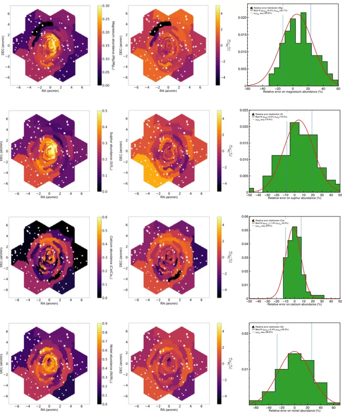
Relative error on iron abundance (%) −30 −20 −10 0 10 20 30 Fig. 3.Left: reconstructed ICM parameters maps for C2 at z ∼ 0.1 using the multi-band fit presented in Sect.4.6with S /N ∼ 300 (∼90 000 counts per spatial bin). Middle: distribution within the regions j of (Pj− Pin,j)/σjindicating the goodness of the fit for each region in terms of σj(see Sect.4.6). Right: relative error distribution across all spectral regions (green histogram). The red solid line pictures the Gaussian best fit. The vertical blue dashed lines are set at the mean value of the fit errors (see Sect.4.6). From top to bottom: spectroscopic temperature Tsl(in keV), emission-measure-weighted abundances of oxygen (O), silicon (Si) and iron (Fe) (with respect to solar).
– Abundance of Ni is finally fitted over the 0.2–12 keV bandpass.
– With all other parameters fixed, redshift, velocity broadening and normalisation are recovered with a broad-band fit. This multi-band post-processing approach is retained in the rest of the paper for local clusters (notably to create Figs.3and4),
along with the comparison of the fitted output temperature with spectroscopic input temperature maps. This technique is used under the caveat that despite some fitted parameters are fixed, errors are propagated correctly throughout the fit. Although not perfectly true, this effect remains very limited with respect to the total systematics and to our level of statistics, ensuring a safe
Relative error distribution (Mg) Best fit (μΔZMg=5.2%,σΔZMg=20.7%) μΔZMg ±μfit (26.6%) 0 0.005 0.010 0.015 0.020
Relative error on magnesium abundance (%) −60 −40 −20 0 20 40 60
Relative error distribution (S) Best fit (μΔZS=4.5%,σΔZS=16.3%) μΔZS ±μfit (14.6%) 0 0.005 0.010 0.015 0.020 0.025
Relative error on suphur abundance (%) −50 −40 −30 −20 −10 0 10 20 30 40 50
Relative error distribution (Ca) Best fit (μΔZCa=-1.4%,σΔZCa=8.3%) μΔZCa ±μfit (8.6%) 0 0.01 0.02 0.03 0.04 0.05 0.06
Relative error on calcium abundance (%) −50 −40 −30 −20 −10 0 10 20 30 40 50
Relative error distribution (Ni) Best fit (μΔZNi=-0.4%,σΔZNi=25.3%)
μΔZNi ±μfit (26.6%)
0.01 0.02
Relative error on nickel abundance (%) −60 −40 −20 0 20 40 60 Fig. 4.As Fig.3, from top to bottom: Magnesium, sulphur, calcium, and nickel abundances (with respect to solar).
application of this method. For all the fitted parameters, we com-puted the mean, µ∆P, and standard deviation, σ∆P, of the relative errors between the output and input values to the mean of the XSPEC fit errors, µfit (see right panels of Figs.3 and4for an illustration in the case of cluster C2) and by computing χ2red for each parameter. Results of this comparison for the main param-eters are given in Table3. In all cases, the mean fit error is con-sistent with the standard deviation of the error distribution σ∆P, thus excluding large systematic effects. However, despite these
changes, small biases of the order of a few percent (/5%) are still visible. This is particularly true for the normalisation and the abundances of low mass elements (e.g. O, Si), in which an underestimate of the normalisation directly results in an overes-timate of these abundances (see also in Fig.3). All these sys-tematics are however well inside the statistical deviations. Using the second test, we notice that some of the χ2
red are not consis-tently recovered, especially for the normalisation. This can be partially explained by the presence of some outlier regions in the
Table 3. Values of the mean µ∆Pand standard deviation σ∆Pof the best fit of the relative error distributions for the main physical parameters in cluster C2, over 80 spatial regions, with the average XSPEC error of the fits µfit. µ∆P(%) σ∆P(%) µfit(%) χ2red χ˜ 2 red Nbad Tsl −0.71 2.60 1.64 3.93 1.38 4 z 0.00 0.04 0.05 1.54 1.09 3 O 4.23 16.0 13.4 1.50 1.50 2 Mg 5.22 20.7 18.4 2.84 1.01 1 Si 3.22 11.4 10.6 1.78 1.37 3 S 4.48 16.3 14.6 1.52 1.41 1 Ca −1.42 8.27 8.62 2.69 1.06 3 Fe 0.94 5.73 5.22 2.71 1.49 2 Ni 0.39 25.3 26.6 0.99 0.92 1 N −6.5 3.68 3.74 4.11 2.83 7
Notes. The corresponding values of χ2
redand the corrected ˜χ 2
redare also given, along with the number of outliers regions Nbadremoved to com-pute ˜χ2
red.
fit, which strongly affect this computation. When the Nbad out-liers regions for which the parameter is outside a 3σfitlevel, are removed, the new reduced chi-squared, ˜χ2red, shows more consis-tency (Table3), indicating a good agreement between the fitted maps and the input distributions.
Small errors remaining after post-processing can be attributed to some degeneracy between fitted parameters (≥15 here) and the spatial binning, which regroups in a relatively large region (a few arcmin2 in the outskirts) many different physical structures (see also the discussion in Appendix B). The choice of a single temperature model could also introduce some bias accounting for the complex structure over the line-of-sight. Two- or multi-temperature models could bring slight improvements, especially towards the centre of the object. Such schemes were investigated over single regions but showed no significant improvement over the entire pointings. The assess-ment of the improveassess-ments introduced by a multi-temperature scheme over the entire temperature distribution as well as the use of line-ratio techniques (Hitomi Collaboration 2018c) will be the object of future improvements of our pipeline, and shall be addressed in future studies. Finally, we also found that small effects related to statistics, to the XSPEC fitting proce-dure, and to the weighting schemes of the input maps par-tially explain these residual deviations (refer to Appendix B
for a more ample and detailed discussion on the pipeline validation).
5. Properties of the ICM of local clusters
In this section we present the results on the ICM properties recov-ered by the X-IFU, starting from the interpretation of the raw out-put maps to larger studies involving the entire cluster sample. 5.1. Physical parameters maps
We show in Fig. 3 the reconstructed maps for cluster C2 at z ∼0.1 for the spectroscopic temperature Tsland the abundances of Fe, Si, and O. Those for Mg, S, Ca, and Ni are shown in Fig. 4. Similar maps for the other three clusters are provided in AppendixC. Beyond the recovery of abundances, the phys-ical parameter maps and their combination provide a wealth of information on the dynamics of the cluster. For instance, we see from the temperature map of cluster C2 the presence of a hot
bubble on the western part of the cluster and a cold arc in the south-eastern region. Interestingly, we also notice the correla-tion between the presence of low-mass elements (e.g. O, Si) and the temperature of the ICM. Several clumps and small groups are also visible on some of the clusters and cluster C3 exhibits a merging activity with a very bright central object. After post-processing, the redshift of each region is also recovered with excellent accuracy from the fit over a large number of lines and spectral features. The redshift map, once converted into veloci-ties using the mean redshift of the cluster, provides a projected map of the bulk motions within the ICM. Likewise, the veloc-ity broadening of the lines is recovered in the fit. Measuring both bulk motion and turbulent velocities through line shifts and line broadening respectively, is another main scientific objec-tive for X-IFU. This, however, goes beyond the scope of this paper and we redirect the reader toRoncarelli et al.(2018) for an illustration.
5.2. Metallicity profiles of the ICM
The hierarchical formation of galaxy clusters along with pro-cesses of production and dispersion of chemical elements within stars and galaxies should lead to self-similar global abundance profiles. The value of the metallicity in the outskirts will depend notably on the enrichment of the intergalactic medium prior to the halo formation (see, e.g.Biffi et al. 2017).
To investigate the capabilities of the X-IFU in determining abundance profiles over the cluster data set, we computed the radial profiles at z ∼ 0.1 for some of the main chemical ele-ments: O, Mg, Si, and Fe (Fig.5). We find that the values of abundance profiles are consistent across the sample, showing a peak near the centre (i.e. up to 0.1 R500) and a decrease towards a constant value between ∼0.1/0.2 Z out to R500. Cluster C3 shows however values of metallicities systematically higher than the others, which could be caused by the ongoing merging activ-ity visible in Fig.1(Bottom left) and possibly due to AGN feed-back. This dynamic activity also creates a more difficult line-of-sight distribution of the parameters, making the XSPEC fit less accurate. This is particularly the case near the outskirts, where background contributions become relevant and regions are large, thus increasing the deviations from the input maps (especially for iron). These measured profiles, and notably their constant metallicity value in the outskirts, suggest as discussed inBiffi et al.(2017),Truong et al.(2018), that the enrichment of the cluster in the hydrodynamical simulations pre-dates the large infall towards the central object and is mainly determined by the early enrichment mechanisms of the Universe. Other indepen-dent hydrodynamical simulations (Vogelsberger et al. 2018) and recent observational results (e.g.Ezer et al. 2017;Mernier et al. 2017; Simionescu et al. 2017) also argue in favour of this paradigm.
Overall, the recovered metallicities are consistent with the input metallicity profiles within 3σ (most well within 1σ), showing the power of the X-IFU in recovering the properties of the ICM even for typical 100 ks exposures. This analysis can be compared to a similar study performed by simulating 200 ks cluster observations with XMM-Newton/EPIC MOS1 and MOS2 for the same chemical species (seeRasia et al. 2008for more details, notably Fig. 4) or to current observational data using the CHEERS catalogue (Mernier et al. 2017). For typi-cal exposure times, the X-IFU will provide accurate measure-ments of the main metallic content of the ICM, enough to reduce the uncertainties on current observations, even for less abun-dant elements. In addition to the individual profiles, the overall
O xyg e n a b u n d a n ce (Z O ) 0 0.05 0.10 0.15 0.20 0.25 0.30 Radius (R/R500) 0 0.2 0.4 0.6 0.8 1.0 C1 C2 C3 C4
Average output abundance ±1σ dispersion Input abundance Ma g n e si u m a b u n d a n ce (Z Mg ) 0 0.1 0.2 0.3 Radius (R/R500) 0 0.2 0.4 0.6 0.8 1.0 Si lico n a b u n d a n ce (Z Si ) 0.1 0.2 0.3 0.4 0.5 Radius (R/R500) 0 0.2 0.4 0.6 0.8 1.0 Iro n a b u n d a n ce (Z Fe ) 0 0.1 0.2 0.3 0.4 Radius (R/R500) 0 0.2 0.4 0.6 0.8 1.0
Fig. 5.Best-fit values of the metallicity as a function of radius, up to R500(0.1 R500 bins) for the entire sample (C1 – purple dots, C2 – orange squares, C3 – green diamonds, C4 – red triangles). From top left to bottom right: oxygen, magnesium, silicon and iron abundances with respect to solar. The dashed lines represent instead the profile of the emission-measure-weighted input abundances using the same colours. The cyan shaded envelope represents the ±1σ dispersion of the recovered output metallicity for the entire sample. Points are slightly shifted for clarity.
dispersion across the sample (Fig.5) is consistent with the aver-age emission-measure-weighted input distribution. However, the sample considered here is relatively small, and the scatter of our results remains significant. Namely, we see that the dynamic behaviour of clusters C3 affects the overall scatter of the sample, otherwise similar for the other three objects (C1, C2, and C4). The values of iron abundance in the outskirts found in this study (between 0.1/0.2 Z ) are somewhat lower than measured iron abundances in the outskirts, which range typically around 0.2 Z (Werner et al. 2013; Mantz et al. 2017; Urban et al. 2017). Values remain however consistent with the hydrodynamical inputs, demonstrating that the X-IFU is able to recover the intrin-sic phyintrin-sical parameters used for the clusters. The projection scheme adopted here also provides lower results than for exam-ple, emission-weighted schemes, in which the strongest emission regions (hotter and/or with more metal) will enhance the overall contribution.
Once in orbit, the X-IFU will probe a much larger number of galaxy clusters (≥10 per mass and redshift bins), therefore
reducing the sample variance of these profiles even further, especially near the outskirts of the clusters. A more accu-rately constrained scatter will provide important information on the metallicity distribution of the ICM and firm observa-tional confirmation of the nature of the enrichment scenario during the early phases of the Universe. These results high-light the sensitivity of the X-IFU to constrain with high accu-racy the chemical enrichment pattern in cluster outskirts, and, therefore, to fully exploit its potential as a fossil record of the star formation history and feedback in the proto-cluster ecosystem.
5.3. Constraints on the chemical enrichment model
As chemical elements are trapped within the ICM, they repre-sent a fossil record of the integrated history of chemical enrich-ment of the cluster. Strong constraints on the relative contribu-tion of the various enrichment mechanisms (notably SNcc and SNIa) could be given by accurate measurements of abundance
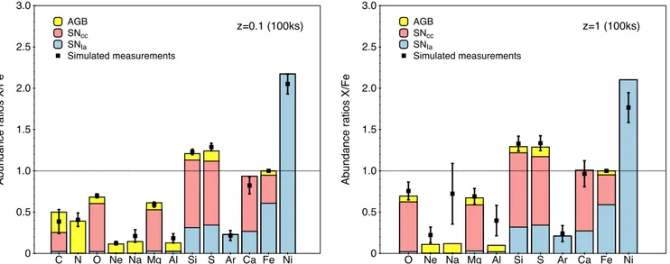
AGB SNcc SNIa Simulated measurements z=0.1 (100ks) Ab u n d a n ce ra tio s X/ F e 0 0.5 1.0 1.5 2.0 2.5 3.0 C N O Ne Na Mg Al Si S Ar Ca Fe Ni AGB SNcc SNIa Simulated measurements z=1 (100ks) Ab u n d a n ce ra tio s X/ F e 0 0.5 1.0 1.5 2.0 2.5 3.0 O Ne Na Mg Al Si S Ar Ca Fe Ni
Fig. 6.Average abundance ratio with respect to iron within R500at z ∼ 0.1 over the cluster sample for z= 0.1 (left) and z = 1 (right) recovered using 100 ks observations. The input abundance ratio are shown as histogram bars filled with the respective contributions of SNIa(blue), SNcc (magenta) and AGB stars (yellow), computed from the outputs of the hydrodynamical simulation presented in Sect.2. For z= 1, carbon (C) and nitrogen (N) are not shown as the lines are outside the energy bandpass of the instrument (not fitted).
Table 4. Mean abundance ratio with respect to iron within R500 at z ∼0.1 for each cluster in the sample.
Cluster 1 Cluster 2 Cluster 3 Cluster 4 C/Fe 0.48 ± 0.34 0.35 ± 0.24 0.43 ± 0.28 0.48 ± 0.31 N/Fe 0.32 ± 0.12 0.40 ± 0.15 0.52 ± 0.30 0.57 ± 0.20 O/Fe 0.73 ± 0.04 0.68 ± 0.04 0.67 ± 0.06 0.69 ± 0.06 Ne/Fe 0.10 ± 0.03 0.12 ± 0.04 0.14 ± 0.06 0.20 ± 0.06 Na/Fe 0.17 ± 0.12 0.34 ± 0.24 0.20 ± 0.13 0.21 ± 0.17 Mg/Fe 0.63 ± 0.05 0.58 ± 0.06 0.59 ± 0.08 0.53 ± 0.08 Al/Fe 0.16 ± 0.08 0.18 ± 0.10 0.21 ± 0.18 0.20 ± 0.13 Si/Fe 1.24 ± 0.06 1.18 ± 0.05 1.27 ± 0.08 1.27 ± 0.09 S/Fe 1.33 ± 0.08 1.30 ± 0.08 1.26 ± 0.12 1.18 ± 0.12 Ar/Fe 0.19 ± 0.09 0.22 ± 0.11 0.20 ± 0.15 0.30 ± 0.17 Ca/Fe 0.94 ± 0.20 0.71 ± 0.16 0.71 ± 0.24 0.99 ± 0.25 Ni/Fe 2.12 ± 0.20 1.91 ± 0.21 2.11 ± 0.29 2.12 ± 0.32 ratios of elements within clusters. Using the small sample at our disposal, we estimated the capabilities of the X-IFU in recov-ering this information in the input hydrodynamical simulations within a radius of R500. A first noticeable result is that for the entire cluster sample, recovered abundance ratios are consis-tent for all the elements (see Table4). Using the average abun-dance ratio profile and the corresponding production yields of each element in the input hydrodynamical simulations, we com-puted the input fraction of each of the enrichment mechanisms (SNcc, SNIa, or AGB) and compared it to the overall output abundance ratio given by our E2E simulations (Fig.6, left). For this study a small fraction of the outlier regions (.5%) was excluded, as results clearly showed incompatible values with respect to emission-measure-weighted inputs for rare elements (N, Na, and Al). All of the elements present in the simula-tions are comparable to the inputs within their statistical error bars. Most of all, the ratios of the main elements of the ICM (e.g. O/Fe, Mg/Fe, and Si/Fe) are very accurately recovered with a significance of the detection ≥10 (i.e. the ratio between the value and the error). Rarer elements (typically Ne, Ar, S, Ca) are also very consistent with the hydrodynamical
simula-tions. Less abundant elements (Na and Al) have looser con-straints in the fitted regions due to the considered exposure time (low S/N of the lines) and seem slightly overestimated in their reconstruction.
With the small sample used here, we have demonstrated that the X-IFU is able to provide robust estimations of the abundance ratios. Given the low errors on the measurements, these results can be used to distinguish the contributions of the various mech-anisms at play in the cosmological simulations, by comparing them to metal production theoretical models. Notably, using ele-ments produced by single mechanisms (e.g. Ne, Na for AGB, or Ar, Ni for SNIa), accurate measurements of abundance ratios will provide strong constraints to the IMF and the contribution of each mechanism at local redshift. The ability to recover the cor-responding supernovæ yield and to distinguish between multiple other models shall be addressed in a forthcoming study. The cur-rent observational strategy of the X-IFU plans to use at least 40 clusters of galaxies to investigate the chemical enrichment of the Universe. With such a large sample and by giving unprecedented information on other rare elements (e.g. Mn, Co, that could not be tested here since these metals are not separately traced in the hydrodynamical simulations), the X-IFU will undoubt-edly provide new constraints to the global chemical enrichment models.
6. Chemical enrichment through cosmic time
Element abundances in local clusters embed the integrated chemical enrichment of the Universe up to this day. However, to understand how and when the ICM was enriched, the evolution of production sources with time and how the overall enrichment processes relate (e.g. the star formation history and the initial mass function) must be assessed. To do so, we analysed syn-thetic observations of the same four clusters taken at different stages of their evolution, hence considering five redshift values up to z= 2. We chose to keep a realistic exposure time fixed to 100 ks, regardless of the redshift. This exercise tested the capa-bilities of the X-IFU in a regime of low statistics, thus preventing the full spatial analysis presented above. For the highest redshift
Fig. 7.From top left to bottom right: maps in number of counts per X-IFU pixel (249 µm pitch) for cluster C2 (see Table1) simulated with the end-to-end simulator SIXTE for redshift z ∼ 0.5 (top left), 1 (top right), 1.5 (bottom left) and 2 (bottom right), for an exposure time of 100 ks.
clusters we complied strictly to the definition of the Athena sci-ence case on chemical abundances and performed measurement in two different annuli from the cluster centre between 0–0.3 R500 and 0.3–1 R500.
Figure7shows the mock surface brightness maps for C2 at the various redshift snapshots and illustrates the assembly his-tory of halos through, for example, merging events. Figure 8
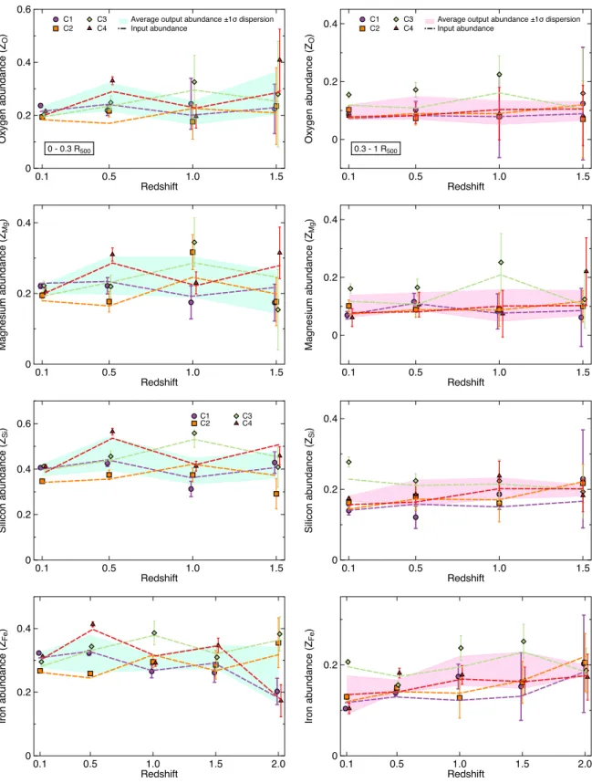
shows the evolution of the mean cluster abundance over our whole sample as a function of the redshift in the two afore-mentioned annular regions for O, Mg, Si, and Fe. Despite the lower source-to-background level of some objects, input metal-licity values are recovered accurately within the statistical uncer-tainties of the measurements even for high-redshift clusters, although for z ≥ 1, error bars start to be significant for elements such as O and Mg. In the case of low-mass elements, abundances are not measurable up to a redshift of z = 2, as lines are red-shifted outside the instrument energy band (e.g. O and Mg for z ≥1.5) or are too weak to be disentangled from the foreground and the background (e.g. Si at z = 2). As expected, measure-ments in the central parts of the cluster are more accurate, due to the higher level of background in the outskirts with respect to the cluster emission, especially for z ≥ 1.5.
Through these measurements, we find that in the central parts of the cluster, metallicity hardly changes across time, even at a redshift of z = 2, once again consistently with the analysis by Biffi et al. (2017). This indicates that most of the enrichment occurs in the early days of the cluster. Interestingly, we notice that the iron abundance in the centre of the cluster slightly decreases with redshift, which could be explained for instance by an increase in time of iron production mechanisms (e.g. SNIa) or by the time delay with which long-lived SNIa release Fe. Abundances in the outskirts show a similar trend, with near-constant values up to local redshift values. Similar observational evidences, as for example, reported inEttori et al.
(2015) for iron abundance are consistent with these conclusions. The dynamic history of the clusters (mergers, shocks) is visible over time (data points are taken from the same cluster at different time steps), displaying local peaks of abundance, for example, C3 at z= 1 or C4 at z = 0.5. Given the sparse number of redshift points, turbulence or mixing within the cluster (whose eddy turn over timescale is of the order of a few Gyr over scales of ∼1 Mpc for typical ∼500 km s−1velocities) create a more homogeneous distribution of metals in the structure, returning abundances to typical values after mergers.
C1 C2
C3 C4
Average output abundance ±1σ dispersion Input abundance 0 - 0.3 R500 O xyg e n a b u n d a n ce (Z O ) 0 0.2 0.4 0.6 Redshift 0.1 0.5 1.0 1.5 C1 C2 C3 C4
Average output abundance ±1σ dispersion Input abundance 0.3 - 1 R500 O xyg e n a b u n d a n ce (Z O ) 0 0.2 0.4 Redshift 0.1 0.5 1.0 1.5 Ma g n e si u m a b u n d a n ce (Z Mg ) 0 0.2 0.4 Redshift 0.1 0.5 1.0 1.5 Ma g n e si u m a b u n d a n ce (Z Mg ) 0 0.2 0.4 Redshift 0.1 0.5 1.0 1.5 C1 C2 C3C4 Si lico n a b u n d a n ce (Z Si ) 0 0.2 0.4 0.6 Redshift 0.1 0.5 1.0 1.5 Si lico n a b u n d a n ce (Z Si ) 0 0.2 0.4 Redshift 0.1 0.5 1.0 1.5 Iro n a b u n d a n ce (Z Fe ) 0 0.2 0.4 Redshift 0.1 0.5 1.0 1.5 2.0 Iro n a b u n d a n ce (Z Fe ) 0 0.2 Redshift 0.1 0.5 1.0 1.5 2.0
Fig. 8.Evolution of the average abundance of the cluster sample (C1 – purple dots, C2 – orange squares, C3 – green diamonds, C4 – red triangles) recovered via XSPEC as a function of the redshift between 0–0.3 R500 (left) and 0.3–1 R500 (right). From top to bottom: oxygen, magnesium, silicon and iron abundances with respect to solar. The dashed lines represent the profile of the emission-measure-weighted input abundances using the same colours. The cyan (resp. magenta) shaded envelope represents the ±1σ dispersion of the output metallicity over the sample. Points are slightly shifted for clarity.
Using the accuracy of the X-IFU abundance measurements for high-redshift objects, we can also analyse changes in the metal enrichment mechanisms by performing a similar study as the one presented in Sect.5.3. In the case of redshift z = 1 (see Fig.6, right) for 100 ks observations, we find that the X-IFU will
still be capable of accurately recovering abundance ratios within R500with excellent accuracy. Most of the main elements have in fact no significant changes between both redshift values, consis-tently with our previous conclusions. In the case of high-redshift objects however, low-mass elements such as carbon and nitrogen
can no longer be detected (lines outside the energy bandpass) and rarer elements (e.g. Ne, Na, and Al) have large uncertainties due to the low S/N of the observations. Ni also tends to be under-estimated (mostly in the outskirts) likely due to the low S/N of the line with respect to the high-energy background. This calls for better-adapted exposure strategies to optimise the results for distant objects and further investigate the chemical enrichment across cosmic time.
7. Summary and discussion
In this paper, we have addressed the feasibility of constraining the chemical enrichment of the Universe, which will be one of the key science objectives and a main driver of the performances of the future mission Athena. Notably, we investigated and quantified the capabilities of the X-IFU in accurately recovering metal abun-dances of the ICM across cosmic time. To this end, we developed a full end-to-end pipeline, which creates synthetic X-IFU obser-vations using the instrument simulator SIXTE. We used as input of this pipeline a sample of four clusters generated using state-of-the-art cosmological simulations presented inRasia et al.(2015) andBiffi et al.(2017) to create realistic event lists. All the rele-vant instrumental effects such as the convolution of spectra with the instrument spatial and spectral responses, realistic sources of foreground and background, and detector geometry were also included to obtain observations as realistic as possible.
The sample of four clusters was simulated at five different redshift values, for a fixed exposure time of 100 ks in order to achieve abundance measurements out to R500. The accuracy of the pipeline was quantified by comparing our synthetic obser-vations to weighted inputs quantities (e.g. spectroscopic temper-ature, emission-measure-weighted abundances). We find that a straightforward approach of a broad-band fit created systematic biases above 10% in a number of physical parameters. Rather a multi-band energy fitting procedure ensured more accurate recovery by optimising the extraction of the several chemical abundances and other physical parameters of interest (notably temperature). After post-processing, distributions are accurately recovered (almost always within the 3σ of the measurement error) with little to no systematic biases (of the order of a 5%, see Sect.4.6) found mainly between the low-mass element abun-dances (e.g. O, Si) and the normalisation. The comparison of the relative distribution between outputs and inputs with respect to the XSPEC statistical error also showed reduced chi-squared val-ues ˜χ2
redclose to 1 when a small fraction of outlier regions (≤5%) is removed indicating a good accuracy in the fits. Remaining errors and biases can be linked to correlation between parameters (notably the normalisation), to the choice of the input weight-ing scheme, and to mixweight-ing effects along the line-of-sight in view of the single plasma temperature model used here. We also find that most of these errors decrease when statistics are strongly increased (biases below 2% at 1 Ms for the same spatial regions), suggesting that these effects may simply be related to statistics (see AppendixB). Studies conducted by decreasing the statistics of the runs (typically by decreasing the S/N of the regions to 50 or 100) provided equally encouraging results. Despite larger sta-tistical errors (up to 10% higher), the main parameters (tempera-ture, redshift, O, Si, or Fe abundance) were accurately recovered. Some fainter lines (e.g. Na, N, or Al) become however very dif-ficult to constrain in this case.
For local clusters (z ∼ 0.1), we demonstrate the power of the X-IFU in accurately recovering spatially resolved parameter maps, along with abundance profiles (Sect.5.2) and abundance ratios (Sect.5.3). The study was then extended at different
red-shift values, up to z ∼ 2. By probing the chemical enrichment for very distant clusters and despite the lack of an optimised obser-vation strategy (i.e. non-optimised exposure time), we also show the power of the X-IFU in investigating the ICM properties and the chemical enrichment of the distant Universe.
The binning and fitting procedures used here comprise “clas-sical” approaches to X-ray data analysis, using S/N binning and fits through instrumental response matrices in XSPEC. Despite our efforts, the fitting procedures remain slightly biased (≤5%) and small changes in the fitting approach can impact the over-all results of the simulation (of the order of a few %). More accurate results may be achieved using, for example, Monte-Carlo (MC) fitting approaches, but unfortunately remain com-putationally cumbersome to be used on our large set of spa-tial regions. More optimised binning techniques could also be investigated for future applications (Kaastra & Bleeker 2016). The access to high-resolution spectra will provide new prox-ies to estimate quantitprox-ies such as the temperature by using for example, line-ratio techniques. Eventually, hyper-spectral meth-ods (e.g. blind source separation algorithms) or machine-learning-based fitting techniques (see, e.g.Ichinohe et al. 2018) could open new perspectives for the post-processing of high-resolution X-ray spectra. We would like to emphasise that, even though not appli-cable in our simulation case, the expected level of spectral resolution ofthe X-IFUwillchallenge ourcurrentknowledge accu-racy of the spectral lines (centroid energies and intrinsic widths). This is critical to allow a meaningful interpretation of the results (as demonstrated inHitomi Collaboration 2018d, for line ratios) and to disentangle fine spectroscopic e ffects(suchasresonantscat-tering,Hitomi Collaboration 2018b). This emphasises the need for dedicated tools able to process and analyse future X-IFU high-resolution spectroscopy data-cube. In this regard, the Athena mission will certainly benefit from the advances expected in pro-cessing tools, fitting methods and atomic databases, from the future XRISM mission (Ishisaki et al. 2018).
Not only do these E2E simulations allow us to explore the capabilities of the future X-IFU instrument, but they also give cru-cial information on the effect of instrumental parameters in sci-ence observations. In this study for instance, the spectral shape of all the foreground and background components were assumed to be perfectly known. For the more local and massive clusters however, the field-of-view of the X-IFU will easily be encom-passed within the angular extension of R500. Cluster emission-free regions might thus be unavailable for local background calibra-tion. The spectral resolution of the X-IFU will help mitigate this effect, by allowing us to disentangle various components through the characteristics of their spectral energy distribution. The instru-ment background may also contaminate the observation of faint sources, as the level of precision to which X-IFU is expected to perform requires its accurate and reproducible knowledge in flight. This may be achieved through, for example, in-flight cross-correlation with the WFI or the X-IFU cryogenic anti-coincidence detector (Cucchetti et al. 2018). Future developments could take advantage of this simulation pipeline to test other realistic instru-mental effects (e.g. stray-light for galaxy cluster outskirts obser-vations). More detailed studies of the abundance ratios recovered here will also be at the centre of a forthcoming study to high-light the capabilities of the X-IFU in constraining the ICM chem-ical enrichment, and notably to disentangle between the contribu-tions of the various mechanisms of chemical enrichment (e.g. SN, AGB) throughout cosmic time.
Our study underlines the revolutionary capabilities brought by the X-IFU in future X-ray spectroscopy. With typical routine observations, the X-IFU will drastically change our