H-INFINITY OPTIMAL CONTROL OF ACTIVE DUMPERS
FOR AUTOMOTIVE SUSPENSION SYSTEMS AND CIVIL STRUCTURES
by Jamal Ezzine
A dissertation submitted to the faculty of Modelling for Engineering University of Calabria
in partial fulfilment of the requirements for the degree of
Doctor of Philosophy
International Doctorate Programme Bernardino Telesio School of Hard Sciences
University of Calabria November 2009
University of Calabria
DEPARTMENT APPROVAL
of a dissertation submitted by Jamal Ezzine
This thesis has been reviewed by the research advisor and research coordina-tor, and has been found to be satisfactory.
Date Prof. A. Casavola and Prof. A. Vulcano, Advisor
H-INFINITY OPTIMAL CONTROL OF ACTIVE DUMPERS
FOR AUTOMOTIVE SUSPENSION SYSTEMS AND CIVIL STRUCTURES
Jamal Ezzine
Department of modelling for engineering Doctor of Philosophy
In recent years the protection of structures against hazardous vibration has gained special interest. Structures such as buildings, bridges and vehicles are subject to vibrations that may cause malfunctioning, un-comfort or collapse. It is an extended practice to install damping devices in order to mitigate such vibrations. Furthermore, when the dampers are controllable, the structure acts as an adaptronic system. Adaptronic systems are characterized by their abil-ity to respond to external loading conditions and adapt themselves to these changes. These abilities can be exploited to solve the vibration mitigation problems through the installation of controllable dampers and the design of appropriate control laws for an adequate actuation. These modern systems in the case of vehicle suspension systems offer improved comfort and road hold-ing in varyhold-ing drivhold-ing and loadhold-ing conditions compared to traditional passive devices.
ACKNOWLEDGMENTS
I would like to express my sincere gratitude to Prof. M. Aristodemo, Prof. A. Casavola and Prof. A. Vulcano who has guided me through out my research activity.
Table of Contents vi
List of Figures ix
1 Introduction 1
1.1 Overview . . . 1
1.2 Problem Definition . . . 1
1.3 The Scope of the Thesis . . . 2
1.4 Structure of the Thesis . . . 3
2 Vehicle Modelling and Dynamics 4 2.1 Introduction . . . 4
2.2 Vehicle Ride Model . . . 5
2.2.1 Vehicle Degrees’s of Freedom (DOF) . . . 6
2.2.2 Types of Suspensions Control System . . . 9
2.3 MR Damper and Parameters Estimation . . . 10
2.3.1 Design of Magneto-rheological Damper . . . 10
2.3.2 Experimental Results . . . 11
2.3.3 Applications of MR Technology in the Industry . . . 13
2.4 Vehicle Motion . . . 15
2.5 Tyre Modelling . . . 16
2.6 Road Modelling . . . 17
2.7 Simple Car Model . . . 20
2.7.1 Quarter-Car Model . . . 21
2.7.2 Half Car Model . . . 23
2.8 Human Body Response . . . 25
2.8.1 Low-frequency Seated Human Model . . . 26
2.8.2 Multy Frequency Input . . . 27
2.9 Passenger Car Model . . . 29
2.9.1 Quarter Car Passenger Model . . . 29
2.9.2 Half Car Passenger Model . . . 31
CONTENTS vii 3 Controller Design 36 3.1 Control Algorithm . . . 36 3.1.1 Optimal Control . . . 36 3.1.2 Predictive Control . . . 40 3.1.3 Robust Control . . . 42 3.2 H∞ Theory . . . 45 3.2.1 Statement of H∞ Control . . . 46
3.2.2 Specifications with Mixed Sensitivity Functions . . . 51
3.3 LMI based Hinf Control Suspensions Car . . . 55
3.3.1 Example Linear Matrix Inequality . . . 55
3.3.2 Some Standard LMI Problems . . . 56
3.3.3 Problem LMI based Hinf Problem . . . 58
4 Simulations Result 61 4.1 Results of simple car model . . . 61
4.1.1 Functions of Weight . . . 61
4.1.2 Results of simple car model . . . 62
4.2 Results of Quarter-Car Model with Passenger . . . 64
4.2.1 Frequency Domain . . . 64
4.2.2 Time domain . . . 64
4.3 Results of Half-car model with passenger . . . 66
4.3.1 Frequency Domain . . . 66
4.3.2 Time domain . . . 69
5 Structural Control in Civil Engineering 70 5.1 Introduction . . . 70
5.2 Classification of Building Control . . . 71
5.2.1 Passive Control . . . 72
5.2.2 Active Control . . . 73
5.2.3 Semi-Active Control . . . 74
5.2.4 Hybrid Control . . . 75
5.3 Actuator Systems for Active and Semi-Active Building Control . . . . 75
5.3.1 Hydraulic Actuation and Active Bracing . . . 75
5.3.2 Hydraulic Actuation and Active Tendons . . . 77
5.3.3 Hydraulic Actuation and the Active Mass Driver . . . 78
5.4 Controllable Fluid Damper . . . 79
5.4.1 Magneto-Rheological Damper Behaviour . . . 80
6 Benchmark Civil Structural Control Problems 85 6.1 Active Control Systems: The LQG Approach . . . 88
6.2 Semi-Active Control Systems: The Clipped Optimal Control Approach 89 6.3 Three-Story Building . . . 91
7 Conclusions and Future Work 96
7.1 Conclusion . . . 96
7.1.1 Automotive Suspension Systems . . . 96
7.1.2 Civil Structures . . . 97
7.2 Future Research Directions . . . 97
7.2.1 Controllable MR Dampers . . . 98
7.2.2 Large-scale Building Problems . . . 98
7.2.3 Nonlinear Building Models . . . 99
A Control Software 100 A.1 Practical Considerations . . . 101
A.1.1 Time Delay and Time Lag . . . 101
A.1.2 Structural Nonlinearities . . . 102
A.1.3 limited Number of Sensors and Controllers . . . 102
A.1.4 Discrete-Time Control Features . . . 103
A.1.5 Reliability . . . 103
B Hardware Description 105 B.1 Active Control Force Generation System . . . 106
B.1.1 Control Device Power Supplier . . . 107
B.1.2 Analog Control Console . . . 107
B.1.3 Active Force Generation device (AFGD) . . . 108
Index 110
List of Figures
2.1 Rear and Front suspension System(Ricambi Tuning). . . . 5
2.2 Vehicle Model (for vertical dynamics only). . . 8
2.3 Magneto-rheological Dampers. . . 10
2.4 Responses of force under different electric currents . . . 12
2.5 Equivalent damping coefficient vs. velocity . . . 13
2.6 Delphis MagneRide (MR)system . . . 14
2.7 Orientation of Axes. . . 16
2.8 Spatial Road Profile (model input). . . 18
2.9 Pseudo-Random Road Profile [GSS+08] . . . . 19
2.10 Quarter-car suspension model [KZ06] . . . 22
2.11 Half-car suspension model [KZ06]. . . 24
2.12 Vehicle and occupant model [GSS+08]. . . . 27
2.13 Quarter-car passenger suspension model [KZ06]. . . 30
2.14 Half-car passenger suspension model [KZ06]. . . 32
3.1 The 2 input and 2 output block problem [CAS01] . . . 47
3.2 The DKGF parameterization of all stabilizing compensator [CAS01] 47 3.3 Mixed sensitivity problem as part of H∞ control problem . . . 53
4.1 Functions of Weighing (Wzs, Wzu, Wzs2, Wu) . . . 62
4.2 QCTF between road profiles y and chassis position x. . . . 63
4.3 QCTF between road profiles y and chassis position ¨x. . . . 63
4.4 QCTF between road profiles y and chassis position x. . . . 64
4.5 QCTF between road profiles y and chassis position ¨x. . . . 65
4.6 Quarter-car, Responses of passenger positions, in Time Domain . . . 65
4.7 HCTF. between road profiles y1 and chassis position x. . . . 66
4.8 HCTF between road profiles y2 and chassis position x. . . . 66
4.9 HCTF between road profiles y1 and chassis acceleration ¨x. . . . 67
4.10 HCTF between road profiles y2 and chassis acceleration ¨x. . . . 67
4.11 HCTF between road profiles y1 and pitch acceleration ¨θ. . . . 68
4.12 HCTF between road profiles y2 and pitch acceleration ¨θ. . . . 68
4.13 Half-car, Responses of passenger positions, in the time response . . . 69
5.1 Passive a, Active b, and Semi-Active c . . . . 72 ix
5.2 Base isolation schematic . . . 74
5.3 Hydraulic actuation and active tendon configuration. . . 77
5.4 Tuned Mass-Damper. . . 78
5.5 Magneto-rheological Dampers . . . 80
5.6 Schematic model of magneto-rheological dampers [SDSC97] . . . 82
5.7 MR force due to a sinusoidal displacement and varying input voltages. 83 5.8 MR force due to a sinusoidal displacement and varying input voltages. 84 6.1 Clipped-Optimal Control Strategy . . . 90
6.2 Three-story building schematic. . . 92
6.3 With a. b.: displacement of the (a) first, (b) second, and (c) third floors. 93 6.4 With a. b.: acceleration of the (a) first, (b) second, and (c) third floors. 94 6.5 With MR: acceleration of the (a) first, (b) second, and (c) third floors. 95 B.1 General hardware function of the active control system. [CAS01] . . 106
Chapter 1
Introduction
1.1
Overview
In recent years, designers of modern vehicle suspensions have begun to seriously con-sider the use of active suspensions due to their potential to improve the ride and road handling quality and better satisfy the structural constraints. Vehicle suspensions also play an important role in protecting chassis and several parts from vibrations and shocks. Their main objectives are the achievement of minimum variations in dy-namic tire loads, good isolation of the chassis from vibration and harshness induced by road unevenness and driving manoeuvres and the stabilization of the chassis during manoeuvres. Most of these new systems equip now luxurious cars.
1.2
Problem Definition
Control of mechanical and civil engineering structures is still an open field and novel theoretical and practical developments must be obtained. Nevertheless, thanks to huge technology advances in areas such as sensing, computation and control important
structural control problems have been solved. Thus, actively controlled suspension systems are now becoming implementable also from economic and reliableness points of view. However, some problems still continue to be open and some others have been appeared with the introduction of innovative suspension systems. For example the introduction of semi-active technologies has produced an important novelty in the field because of their low-energy actuation requirements and maintenance costs. How-ever, more complex control problems have results for their slow responses, low control authority and for the presence of highly nonlinear behaviours due to their intrinsic hysteresis. Thus, one of the challenges in suspension control and civil structural control is that of finding adequate control laws that accomplish minimal design spec-ifications such as robustness, reliability, stability, implementability, minimum control effort, but additionally be able to take into account some particular conditions of the suspension and structural systems, such as actuator dynamics, parametric uncertain-ties, resonance conditions, non-lineariuncertain-ties, coupling and limited measurements.
1.3
The Scope of the Thesis
The problem considered in this thesis is the design and the analysis of control strate-gies for active suspensions in road vehicles, based on H∞ optimal control theory. The
main focus of the study is the improvement of the vibration isolation while driving on a rough terrain. The vibration level is closely related to the discomfort of the driver and passengers. Vehicle suspensions serve several conflicting purposes, in addition to counteracting the body forces resulting from cornering, acceleration, or braking and changes in payload. Suspensions must isolate the passenger compartment from road irregularities. In this thesis, we decided to study the control of vibration on two types of car modes: first, the one which considers the presence of passengers in
1.4 Structure of the Thesis 3 the control scenario and second without passengers. In both cases, quarter-car and half-car dynamical models will be considered. Also, the application of active control on civil structures will be investigated.
1.4
Structure of the Thesis
This doctoral thesis is organized in five chapters. The first one includes an intro-duction, the motivations and the main objectives of the thesis. Chapter 2 describes the types of vehicle models and dynamic behaviours considered. Quarter-car and half-car models, with and without the dynamic of the passenger bodies, will be fully detailed. Further, H∞ optimal control is described and its application to our model
is presented, which results one instance of a H∞ mixed sensitivity control problem,
in Chapter 3. Simulation results on significant tests are therefore presented and used to pointing out the improvement achievable, over passive suspension systems, by the use of active technology in Chapter 4. Chapter 5 presents various structural control problems in Civil Engineering. Finally, Last Chapter will conclude this dissertation.
Vehicle Modelling and Dynamics
In this chapter the model used for the remainder of this thesis will be introduced, along with its equations of motion and the state space formulation. Once the model is established, it is used to investigate vehicle dynamics for various loading cases and disturbances. This investigation provides fundamental justifications for the research presented in this thesis.2.1
Introduction
Conventional suspension design is inherently complex and consists of a trade-off, see Figure 2.1, primarily between ride quality and road handling. In addition to this compromise, passive suspension system performance deviates greatly as the vehicle mass varies. Active suspension techniques seek to improve both ride and handling over a wide range of operating conditions. However, a new set of compromises must be traded-off, as active suspension systems increase system complexity and the consume of vehicle power. Nonetheless, active suspension control promises a leap in suspension performance over its passive counterpart. In the following sections, background
2.2 Vehicle Ride Model 5 formation on the common vocabulary used, notation and assumptions made in active suspension development is introduced. Then, the current state of the art of models and control techniques used for active suspension control is reviewed.
Figure 2.1 Rear and Front suspension System(Ricambi Tuning).
In terms of development of suspension systems, the most relevant factor that leads to degradation of ride quality is the disturbance from the roughness of the road. There are many ways to classify road disturbances, but usually they are divided into two main classes, vibration and shock. Shock is described by a relatively short duration, high intensity event, such as a pothole or speed bump. Vibration is characterized by prolonged, relatively consistent low amplitude excitations, the typical road rough-ness. Obviously, a suspension system must be able to cope with both types of road conditions, in addition to any handling requirements during turning.
2.2
Vehicle Ride Model
A broad variety of vehicle mathematical models of increasing degree of complexity has been developed over the years by automotive engineers to provide reliable models
for computer-aided automotive design and vehicle performance assessment.
From a purely mathematical standpoint vehicle models can be categorised as dis-tributed models governed by partial differential equations and lumped parameter models governed by ordinary differential equations [GSS+08]. The former are mainly
of interest to vehicle design rather than control algorithm design. Distributed models (typically solved numerically with finite-element-based methods) are widely employed in mechanical, thermal, aerodynamic analyses as well as crash-worthiness analyses. For car dynamics (ride and handling) and control studies, lumped parameter models are usually employed. They typically aim to model either ride or handling dynamics or both. In this thesis only lumped parameter models will be considered. A car can be thought as being composed of two main subsystems: the sprung mass (chassis) and the unsprung masses (wheels, axles and linkages), connected via a number of elastic and dissipative elements (suspensions. tyres etc.) and subjected to external inputs coming from the road profile, the steering system and other external disturbances (e.g., wind gust).
2.2.1
Vehicle Degrees’s of Freedom (DOF)
The motion of a vehicle with the nonholonomic constraint of the road has six degrees of freedom (6DOF), classified as follows:
longitudinal translation (forward and backward motion) lateral translation (side slip)
vertical translation (bounce or heave) rotation around the longitudinal axis (roll) rotation around the transverse axis (pitch)
2.2 Vehicle Ride Model 7 rotation around the vertical axis (yaw)
Vehicle ride is essentially concerned with car vertical dynamics bounce, pitch and roll whereas handling is concerned with lateral dynamics (side slip, yaw, roll). Ride models are typically composed of interconnected spring-mass damper systems and de-fined by a set of ordinary differential equations. The most trivial representation of a vehicle suspension has 1 DOF. In this simple model the chassis (body) is represented by a mass and the suspension unit by a spring and a damper. Tyre mass and stiffness are neglected as well as any cross-coupling dynamics. By incorporating a wheel into the model, a more accurate representation having 2 DOF (typically referred to as a quarter car model) can be developed. This model was (and still is) very popular in the automotive engineering community, especially before the widespread use of com-puter simulation, the reason being that the quarter car model, despite its simplicity, features the main variables of interest to suspension performance assessment: body acceleration, dynamic tyre force and suspension working space [SH86]. A merit of the quarter car is that it permits to evaluate more straightforwardly the effects of modifi-cations in control parameters because higher-order dynamics and cross-coupling terms with the other suspension units are not taken into account. A good suspension design should produce improvement of both vehicle road holding and passenger comfort (or possibly improvement of one without degradation of the other), although inherent trade-offs are unavoidable in the design of a passive suspension system.
The quarter car is a 2 DOF system having two translational degrees of freedom. Another classical model can be obtained with only 2 DOF: the half vehicle model hav-ing a translational degree of freedom and a rotational degree of freedom to describe, respectively, bounce and pitch motions or, analogously, bounce and roll motions (in the former case the model is referred to as a bicycle model). Its natural extension is a 4 DOF model, which also includes tyre masses and elasticity. This model can be
Figure 2.2 Vehicle Model (for vertical dynamics only).
employed to study the vehicle pitch (or roll) behaviour. However, the 4 DOF model cannot take into account the cross-couplings between the right- and left-hand side of the car (or front and rear in the case of roll motion). These interactions can be taken into account only by using a 7 DOF mode (sometimes referred to as a full car model) see Figure 2.2 , which allows one to represent bounce, roll and pitch motions. The models mentioned above are classical ride models. Higher order ride models can be developed including further degrees of freedom, e.g., accounting for seat and engine mounting elasticity. Driver and passengers can be modelled as well with springs, masses and damping elements. This is particularly important for accurate human comfort studies. Analogously to ride vehicle models, also handling models having different degrees of complexity can be developed. The equivalent handling model of the quarter car is a linear single track model which describes lateral and yaw dy-namic responses to handling manoeuvres (ignoring the effect of sprung and unsprung masses).
Models including both ride and handling dynamics are necessary when there is a need to accurately investigate the interaction between ride and handling (during
2.2 Vehicle Ride Model 9 a turning manoeuvre, for instance) and to study the limit of handling characteris-tics or elements such as anti-roll bars. Multi body techniques allow relatively easy development of complicated models with many degrees of freedom.
Analogously to cars, several heavy and trailed vehicles tractor and/or semi-trailer models [SH86] and [Won08] have been developed to examine their ride comfort, tractort/railer interactions, dynamic tyre forces and road damage. A survey can be found in [JSEG01]. These vehicle models usually include linear tyre models, linear or nonlinear suspension characteristics, tandem or single axles. Other truck ride models include suspended tractor cab and driver seat with linear or non-linear components. The models described and the simulation results presented in this thesis are based on the use of MATLAB and Simulink software.
2.2.2
Types of Suspensions Control System
Additional areas of confusion with terminology include the distinction amongst: pas-sive, semi-active and active suspension systems.
passive systems are classified as those that are only able to dissipate energy and
that require no external energy sources to operate.
Fully active systems are classified as those that supply energy to the systems,
generally in the form of a force generating element in parallel to, or in place of, the passive suspension components.
Semi-Active systems are classified as those that vary system parameters, but do
not supply energy to the suspension system itself; these systems are only able to dissipate energy.
Semi-active systems are essentially variable dampers or springs. Semi-active sys-tems do require external power, but far less than their fully active counterparts. To
see this, consider the power needed to vary the orifice size on a variable damper, to the power needed to move the suspension through its operating range. And for that we are decide to illustrate the feature of MR Controllable Damper.
2.3
MR Damper and Parameters Estimation
Most active suspension systems in production today are of semi-active type, so we are going to show the similarities of the Design of semi-active MR damper see also 5.4 .
2.3.1
Design of Magneto-rheological Damper
Figure 2.3 Magneto-rheological Dampers.
The prototype MR damper works in flow mode as shown in Figure 5.5. The damper is 218 mm long in its extended position, and has ± mm stroke. The main cylinder houses a piston, a magnetic circuit, an accumulator and MR fluid. MR 132 LD, which was obtained from Lord Corporation, is used in the damper [Htt]. The MR fluid valve is contained within the piston and consists of an annular flow channel with 1.5 mm gap. The magnetic field is applied radially across the gap, perpendicular to the direction of fluid flow. The total axial length of the flow channel is 6 mm which exposed to the applied magnetic field. Viscosity of MR fluid in the
2.3 MR Damper and Parameters Estimation 11 valve will be increased by increasing the electric current through the electromagnet, thus resisting the MR fluid flow through the valve and increasing the damping force of the MR damper. The resistance of the electromagnet coil is 19 Ω.
To apply the MR damper in vibration control of vehicle suspension system, the property of the damper should be determined first and then a model must be devel-oped that can accurately reproduce the behaviour of the MR damper. An experimen-tal test rig is set up to determine the property of the MR damper and to obtain the dynamic data necessary for estimating the parameters of the model. In this test rig, the MR damper is fixed in a computer-controlled INSTRON Test Machine (Model 8874). The INSTRON Test Machine incorporates a load cell and a displacement sen-sor to measure the force produced by the MR damper and the displacement of the piston. Two types of excitations, sinusoidal and triangular, are used. The excitation frequencies are 1, 2 and 4 Hz and the amplitudes of excitation are 1, 2 and 4 mm, respectively. The applied electric current is from 0 to 1 A with increment of 0.25 A. The force and displacement responses of the damper are sampled simultaneously by the computer via an A/D converter. The excitation signal is also produced by the computer and sent out to the hydraulic actuator via a D/A converter. Velocity response can be obtained by differentiating the displacement. All experiments are carried out at the room temperature of 23 .
2.3.2
Experimental Results
The responses of MR damper at 1 Hz excitation under five constant electric currents are shown in Figure 2.4. The effect of magnetic field on the damping force is clearly shown in these figures. With the increasing of the applied electric current, the damp-ing force will increase remarkably, however when the applied electric current is more than 0.75 A, the increase of the damping force is no longer significant. This means
(a) Responses of force vs. time (b) Responses of force vs. displacement
Figure 2.4 Responses of force under different electric currents
that saturation of the MR effect occurs at 0.75 A. It is also noted that the force pro-duced by the damper is not exactly centred at zero. This is due in part to the presence of an accumulator in the MR damper, which is filled with highly compressed air, and in part due to the existence of air in the cylinder since the damper cannot be fully filled with MR fluid. The maximum force of MR damper at 1 A is approximately equal to eight times of that without electric field. Similar results can be obtained from experiment at the other excitation frequencies and amplitudes. To obtain the relation of equivalent damping coefficient to velocity and electric current, experiments are done under the triangular excitation. The equivalent damping coefficient of the damper against velocity under various electric currents is shown in Figure 2.5. It is seen that at low velocity, equivalent damping coefficient will increase markedly. As the velocity increases, the equivalent damping coefficient under high electric current decreases rapidly whereas that without electric current decreases slowly. At high ve-locity, the effect of current on equivalent damping coefficient is also not so significant. This phenomenon means that the MR damper cannot be treated as a viscous damper under high electric current.
From the experiments, it is seen that the designed MR damper has very large changeable damping force range under magnetic field, although the saturated
mag-2.3 MR Damper and Parameters Estimation 13
Figure 2.5 Equivalent damping coefficient vs. velocity
netic field is not so big. An improvement should be proposed to increase the saturated magnetic field and to avoid the side effect of the accumulator. Furthermore since the MR damper cannot be treated as a viscous damper under high electric current, a suitable model is necessary to be developed to describe the MR damper.
2.3.3
Applications of MR Technology in the Industry
Lord Magneto-Rheological (MR) technology enables new levels of performance in automotive primary suspension systems. In an MR suspension, controllable MR fluid replaces traditional hydraulic fluid in each shock absorber. As sensors monitor road and vehicle conditions, a controller modifies the damping characteristics up to one thousand times per second. This enables dramatic improvements in both ride comfort and handling.
Delphis MagneRide system incorporates LORD MR fluid to provide real-time optimization of suspension delphi.jpgdamping characteristics [?]. MagneRide is in-credibly flexible it can be used to improve the driving characteristics of any vehicle, from high-end sports cars, to sedans and SUVs. First introduced in the 2002 model year, the system now appears on more than a dozen models from a wide variety
Figure 2.6 Delphis MagneRide (MR)system
of OEMs, including: Acura MDX, Audi TT,Audi R8,Buick Lucerne, Cadillac DTS,
Cadillac SLR, Cadillac SRX, Cadillac STS, Chevrolet Corvette, Ferrari 599GTB, Holden HSV Commodore.
LORD MR Technology Advantages
Our controllable MR damping technology outperforms all existing passive and active suspension systems.
Unequaled shock and vibration control Lord MR systems offer unsurpassed effectiveness in precise, real-time control of mechanical systems, resulting in an un-equaled ride experience. LORD MR-based suspensions are a no-compromise sus-pension solution that provides both firm cornering and superior isolation from road shocks and vibrations.
Fewer moving parts, less manufacturing complexity Delphis MagneRide shocks with LORD MR fluid have fewer moving parts than conventional controllable shocks 60 percent fewer parts than valve-based semi-active damper systems.
2.4 Vehicle Motion 15 Low power consumption Lord MR suspension systems typically require very little power. In the MagneRide system, peak power is 20 watts at each of the system’s four dampers.
Quieter operation Lord MR dampers are also quieter in operation than those based on conventional servo-valve technology.
Durability-tested and approved Our MR technology has surpassed all automo-tive durability testing for primary suspension shocks and is endorsed by two leading component manufacturers. The durability of this technology is further validated by more than five years of production and billions of incident-free road miles in Class 8 vehicle seat suspensions.
2.4
Vehicle Motion
Vehicle motion is described in a standard way as well. These motions and the relative axes are shown in Figure 2.7. The vertical motion of the sprung mass is referred to as heave, and is usually measured at the sprung mass center of mass. The rotational motion along an axis parallel to the vehicle axles is referred to as pitch. Nose-dive during vehicle braking is an example of the excitation of pitch motion. Roll is ro-tational motion about an axis that spans the length of the vehicle. One roll motion excitation source is cornering. Angular motion about an axis perpendicular to the ground is called yaw. Excessive yaw results in vehicle spin-out.
Figure 2.7 Orientation of Axes.
2.5
Tyre Modelling
Tyres are made of rubber, i.e., a viscoelastic material and usually, in ride studies, the vertical tyre stiffness is approximated by a spring and some damping, either pure viscous or hysteretic damping, but often negligible. The tyre is represented as a spring plus a viscous damping term. This model, although quite crude, is acceptable for ride analysis. Handling, braking or traction studies require more sophisticated models which account for road-tyre adhesion along both longitudinal and lateral axes as well as rolling frictions.
The majority of studies utilise a point contact model since it is easy to use. Such a model has at least two defects. Firstly, the point follows the slightest vertical excursion of the road and hence generates high-frequency inputs which in practice would not occur as the tyre contact patch bridges or envelops such points.
For on-road applications, it is valid to regard the road profile as rigid compared to the flexible tyre. The main difficulty is locating the point of contact for each spring when a pseudo-random road profile is assumed. Such a model generates longitudinal forces but does not admit enveloping, although [Dav75] has extended the model to allow it. Torsional tyre distortion is usually not modelled.
2.6 Road Modelling 17
2.6
Road Modelling
The representation of the road profile is vital for vehicle dynamic simulations because it is the main source of excitation. An accurate road model is as important as a good vehicle model. Sources of vehicle vibration include forces induced by road surface irregularities as well as aerodynamic forces and vibration that arise from the rotating mechanical parts of the vehicle tyres, engine and transmission [GSS+08]. However,
the road surface elevation profile plays the major rule. Road roughness includes any type of surface irregularities from bump and potholes to small deviations. The reduction of forces transmitted to the road by moving vehicles is also an important issue responsible for road damage. Heavy-vehicle suspensions should be designed accounting also for this constraint.
Road inputs can be classified into three types:
Deterministic road, periodic and almost-periodic inputs. Random-type inputs.
Discrete events such as humps and potholes.
As far as deterministic inputs are concerned, a variety of periodical waveforms can be used, such as sine waves, square waves or triangular waves. To a first approximation the road profile can be assumed to be sinusoidal. Although not realistic, it is useful in a preliminary study because it readily permits a comparison of the performance of different suspension designs both in the time and in the frequency domain through permissibility charts, plotted at different frequencies.
A multi-harmonic input which is closer to an actual road profile can be gen-erated. A possible choice which approximates fairly well a real road profile is a
so-called pseudo-random input [Duk00] which results from summing several non-commensurately related sine waves (i.e.. the ratio of all possible pairs of frequencies is not a rational number) of decreasing amplitude, so as to provide a discrete approx-imation of a continuous spectrum of a random input. The trend can be proved to be non-periodic, sometimes referred to as almost periodic in spite of being a sum of periodic waveforms [Duk00]. To achieve a pseudo-random profile effect it is advisable to select spatial frequencies of the form:
j4Ω + transcendentalterm j = 1, ...., m. (2.1) where j is an integer, 4Ω is the separation between spatial frequencies and the added term could be e/1000 or π/I000 for example. The spatial frequency range is (m − I)4Ω). The RMS amplitude at each centre frequency is obtained from the power spectral law and multiplication by 4Ω.
Figure 2.8 Spatial Road Profile (model input).
Another possible way to generate a realistic multi-harmonic input consists in mak-ing the ratio between frequencies constant and decreasmak-ing with amplitude, by usmak-ing randomly generated phase angles between 0 and 360 degrees for each component. In this case, the resulting waveform is periodical. Simulation results presented
subse-2.6 Road Modelling 19 quently are based on the latter approach.
Figure 2.9 Pseudo-Random Road Profile [GSS+08] .
Figure 2.9 shows an example of road profile: 20 sine waves with random phases have been added together in order to create a pseudo-random profile. The amplitude of the profile is calculated to approximate a smooth highway by using the spatial frequency data suggested by the Society of Automotive Engineers (SAE).
However, these road profiles are deterministic functions and as a consequence could not represent a real random pavement. A stochastic model gives the more realistic representation of a road profile. The power spectral density (PSD) is the most common way to characterise the road roughness, a road could well be approximated [Won08] by an ergodic process with spectral density expressed by:
S(Ω) = CΩ−n (2.2)
of wavelength), C is a coefficient dependent on the road roughness, f the frequency in Hz and n is a rational exponent see Figure 2.8 . It follows that Ω = f /V where
V is the forward speed of the car, so that:
S(f ) = ( C V−n)f
−n (2.3)
This approach involves an analysis in terms of power spectral densities. For a linear system the input and output spectral densities Yin(f ) and Yout(f ) are related
through the transfer function of the system G(f ), from the equation:
Yout(f ) = |G(f )|2Yin(f ) (2.4)
This property in the frequency domain only applies to linear systems and allows the output spectral density to be readily calculated if the vehicle transfer function and the input spectral density are known. For a non-linear system this property does not hold true.
2.7
Simple Car Model
Many metrics have been introduced for evaluating ride comfort including root mean square (RMS) vertical acceleration, (RMS) jerk (derivative of acceleration), frequency dependent or weighted accelerations, and rotational accelerations. Most active sus-pension researchers agree, however, that RMS acceleration is an adequate measure to quantify the improvements possible through active suspension control. Additional justification for using only RMS vertical acceleration was found by [Gil92].
About the choice of the type of model there are many different considerations. Many models only deal with vertical motions and cannot take into account the pitch, roll and yaw motions [LRG01]. Half-car pitch-plane models (bicycle models) are
2.7 Simple Car Model 21 often considered to perform good handling capabilities (steering control). However they do not include roll motions. Finally, some papers study complete vehicle model but the four suspension elements are assumed to be independent which is not the case in most vehicles. We will use quarter- and half-car models just for comparison between them, with and without consideration of the passengers dynamics in the simulation.
2.7.1
Quarter-Car Model
It is useful to introduce the vocabulary that will be used throughout the remainder of this thesis. These terms can be introduced in the context of the quarter-car model shown in Figure 2.10. The mass supported by the vehicle suspension is referred to as the sprung mass. All other vehicle mass, which includes all suspension components, vehicle axle assemblies, and vehicle tires and wheels is referred to as unsprung mass. A typical ratio of sprung to unsprung mass is 10:1 see [Gil92]. This ratio will be used for the unloaded cases throughout most of the work here.
The quarter-car has been for a long time been the most used model in suspension design. It is very simple as it can only represent the bounce motion of the chassis and wheel without taking into account pitch or roll vibration modes. However, it is very useful for a preliminary design: it is described by the following system of second-order.
A two-degree-of-freedom quarter-car model is depicted in Figure 2.10 In this model, the sprung and unsprung masses corresponding to the one corner of the vehicle are denoted, respectively, by m and mt. The suspension system is represented by a
linear spring of stiffness k and a linear damper with a damping rate c, whereas the tire is modelled by a linear spring of stiffness kt and linear damper with a damping rate
Figure 2.10 Quarter-car suspension model [KZ06] .
The excitation comes from the road irregularity y. The model is generally reputed to be sufficiently accurate for capturing the essential features related to discomfort, road holding, and working space [Gob01]. The linear equations of motions of the system model are:
¨ x = −1 m(k)x + 1 mkxt+ 1 mc ˙xt− 1 mc ˙x + F m (2.5) ¨ xt = 1 mt (kx − (k + kt)xt+ kty − F ) + 1 m(c ˙x − (c + ct) ˙xt+ ct˙y) (2.6)
The equations of motion of the suspension system can be written in compact form as:
˙z = Az + Bu + Gw (2.7)
where the state vector z, is given by:
z = [x xt ˙x ˙xt]T (2.8)
2.7 Simple Car Model 23
w = [y ˙y]T (2.9)
and the vector u represents the damper forces:
u = [F ]T (2.10)
The matrices A ∈ R4×4, B ∈ R4×1, andG ∈ R4×2
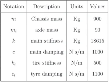
Table 2.1 Quarter Car Suspension Parameters. Notation Description Units Values
m Chassis mass Kg 900 mt axle mass Kg 90 k main stiffness Kg 18615 c main damping N s/m 1000 kt tire stiffness N/m 500 ct tyre damping N s/m 1100
2.7.2
Half Car Model
Figure 2.11 shows a half-car model, which has four degrees of freedom. The model consists of the chassis and two axles. It is assumed that the chassis has both bounce and pitch and the axles have independent bounce oscillations. The suspension and tyre are modelled using linear springs in parallel with viscous dampers [TE98]. Two MR dampers are used to provide controllable forces, and are located parallel to the suspension springs and shock absorbers. To derive the equations of motion for the half-car, the notation given in table 2.4 is adopted. The four degrees of freedom are:
x (vertical displacement of the chassis),θ (rotational displacement of the chassis), xt1
(vertical displacement of tyre 1), and xt2 (vertical displacement of tyre 2).
Summing up all forces acting on all masses and moments about the center of gravity of the chassis leads to the following equations:
¨ x = −1 m(k1+ k2)x − 1 m(k1b1+ k2b2)θ + k1 mxt1+ k2 mxt2 − 1 m(c1+ c2) ˙x − 1 m(c1b1− c2b2) ˙θ + F1+F2 m ¨ θ = −1 Ip (k1b1+ k2b2)x − 1 Ip (k1b21+ k2b22)θ − k1b1 Ip xt1 + k2b2 Ip xt2− c1b1 Ip ˙xt1+ c2b2 Ip ˙xt2− 1 Ip (c1b1− c2b2) ˙x − 1 Ip (c1b21+ c2b22) ˙θ + 1 Ip (F1b1+ F2b2) ¨ xt1= 1 mt1 (k1x + k1b1θ − (k1+ kt1)xt1y1− F1) + 1 mt1 (c1˙x + c1b1˙θ − (c1+ ct1) ˙xt1+ ct1˙y1) ¨ xt2= 1 mt2 (k2x + k1b2θ − (k2+ kt2)xt2y2− F2) + 1 mt2 (c2˙x + c2b2˙θ − (c2+ ct2) ˙xt2+ ct2˙y2) (2.11)
Figure 2.11 Half-car suspension model [KZ06].
The equations of motion of the suspension system can be written in compact form as:
2.8 Human Body Response 25
˙z = Az + Bu + Gw (2.12)
where the state vector z, is given by:
z = [x θxt1 xt2 ˙x ˙θ ˙xt1 ˙xt2]T (2.13)
The vector w represents the road disturbance:
w = [y1 y2 ˙y1 ˙y2]T (2.14)
and the vector u represents the damper forces:
u = [F1 F2]T (2.15)
The matrices A ∈ R8×8, B ∈ R8×2, andG ∈ R8×4
2.8
Human Body Response
The apparent mass resonance frequency is in the range 5.4Hz to 4.2Hz as the mag-nitude of vibration increased from 0.25m/s 102.5m/s. Various detailed models of the human body exist [GSS+08]. However, cushion and visceral natural frequencies are
below 6Hz. Moreover, because the amplitude of road profile fluctuations falls with decreasing wavelength, road inputs experienced by vehicle occupants are predomi-nantly at low frequency. For realistic vehicle speeds higher frequency inputs are not important until wheel-hop is experienced at around 12Hz for cars and near 10 Hz for freight vehicles. When traversing rough ground drivers instinctively slow, reducing the frequency of input.
Table 2.2 Half Car Suspension Parameters. Notation Description Units Values
m Chassis mass Kg 1794
mt1 front axle mass Kg 87.15
mt2 rear axle mass Kg 140.04
Ip Chassis inertia Kg m2 3443
k1 front main stiffness Kg 66824.0
k2 rear main stiffness Kg 18615.0
c1 front main damping N s/m 1190
c2 rear main damping N s/m 1000
kt1 front tire stiffness N/m 500
kt2 rear tire stiffness N/m 500
ct1 front tyre damping N s/m 1190
ct2 rear tyre damping N s/m 1000
b1 distance m 1271
b2 distance m 1713
2.8.1
Low-frequency Seated Human Model
The model adopted for the human body is one of those developed by [WG98]. This is shown in the upper part of Figure 2.12. The non-linear spring Kv models the
stiffness effects with hysterical effects providing damping.
The motion of the visceral mass Mv is denoted by x, and that of the remainder Mc
of the body by y. This second mass could be that of the skeleton. The authors also produced a two-degree-of-freedom model in order to model response at frequencies greater than about 8Hz [GSS+08]. Vehicle simulations using this model indicated
2.8 Human Body Response 27
Figure 2.12 Vehicle and occupant model [GSS+08].
no significantly different response for realistic road inputs and vehicle speeds. Hence the single-degree-of freedom model is adopted here.
The seat is modelled as a mass Ms and a (non-linear) spring Ks. As indicated
above the damping terms are deduced from a hysteric model. A seat control force
Fc is considered. This would be provided by an actuator fixed to the vehicle floor
beneath the seat.
The sprung mass Ms, on a spring and damper suspension, is modelled because
it acts as a low-pass filter of road inputs. In the frequency range of interest, the unsprung mass is neglected as it is common with truck models. [in his experimental work using vertical inputs indicates a natural frequency of the human body in the range 4.2 − 5.4Hz, depending on the amplitude of input [MG00].
2.8.2
Multy Frequency Input
Vehicle-occupant model for low-frequency vibrations is depicted in Figure 2.12. Ground input is indicated by zg. The unsprung mass is not modelled as at the
vehi-cle, restrained by a linear spring and viscous damper. The cushion is modelled as a complex spring Kc with loss factor βc; Mc and Mv, represent the two masses of the
Wei and Griffin 1 DOF model [Wei98], with Kv a non-linear spring with loss factor
βv.
The equations of motion for an input zg of frequency ω are:
¨ x = ω2 vu(1 − ²vu2) + ωv2βv˙u (1 + ²v ˙u 2 ω2) ω ¨ y = −R¨x + (R + 1)ω2 cw(1 − ²cw2) + (R + 1)ωc2βcw˙ (1 + ²vw˙ 2 ω2) ω + Fc Mc ¨ z = ω2s(zg − z) + 2ζωs( ˙g − ˙z) − Fc Mc (2.16) where u = y − x, w = z − y and R = Mv
Mc; ωv is the natural frequency of the linear
visceral system. ωc is the natural frequency of the total mass Mv + Mc on the linear
cushion. ωs is the natural frequency of the sprung mass on its suspension. zg is the
road surface displacement as experienced by the vehicle [GSS+08].
The damping can be calculated by summing the contributions obtained from Indi-vidual frequency inputs [Wet97]. However, this procedure requires the amplitude of vibration at each frequency to be known, calling for a continuous FFT of the response. This would not appear practical and would certainly add expense to the system. The somewhat less elegant solution of selecting a typical ω is the strategy adopted here. The power: the spectral density for the road is defined over a range [Ω1, Ω2] of the
spatial frequency Ω (cycles/m), the frequency (Hz) experienced by a vehicle moving at speed V is V Ω. The excitation has the form
X
ajsin(2πΩjV t + ϕj)
where Ωj is a spatial frequency (cycles/m). V the vehicle speed and ϕj a random
2.9 Passenger Car Model 29
X
aj2πΩjV cos(2πΩjV t + ϕj)
of the road surface displacement. This model can be used to obtain the frequency response of the system, be it passive or controlled.
2.9
Passenger Car Model
Two different others models will be used in this thesis: one is based on a Quarter Car Passenger Model and the other on the Half Car Passenger Model, but in this case we decided to take in consideration not just the model of vehicle but also the passengers inside the vehicle. The models are derived with values and dimensions obtained from a virtual prototype based on a real vehicle [KZ06].
2.9.1
Quarter Car Passenger Model
Quarter-car models with passengers consist of the wheel, unsprung mass, sprung mass, seats with passengers and suspension components (see Figure 2.13). Wheel is represented by the tire, which has the spring character. Wheel weight, axle weight and everything geometrically below the suspension are included in unsprung mass. Sprung mass represents body or in other words, chassis of the car. Suspensions consist of various parts. This model has been used extensively in the literature and captures many essential characteristics of a real suspension system. The equations of motion of the suspension system are:
¨ x = −1 m(k + kp)x + 1 mkpxp+ 1 mkxt+ 1 mcp˙xp+ 1 mc ˙xt− 1 m(c + cp) ˙x + F m (2.17) ¨ xt = 1 mt (kx − (k + kt)xt+ kty − F ) + 1 m(c ˙x − (c + ct) ˙xt+ ct˙y) (2.18) ¨ xP = 1 mP (kPx − kPxP) + 1 mP (cP˙x − cP˙xP) (2.19)
x is the position of the vehicle body center of gravity, xt is the position of the
wheel, xpis the position of passenger and y is the displacements of the road see Figure
2.13. These differential equations can be rewritten in the compact form:
Figure 2.13 Quarter-car passenger suspension model [KZ06].
˙z = Az + Bu + Gw (2.20)
where the state vector z, is given by:
z = [x xp xt ˙x ˙xp˙xt]T (2.21)
The vector w represents the road disturbance:
2.9 Passenger Car Model 31 and the vector u represents the damper forces:
u = [F ]T (2.23)
The matrices A ∈ R6×6, B ∈ R6×1, andG ∈ R6×2
Table 2.3 Quarter Car Passenger Suspension Parameters. Notation Description Units Values
m Chassis mass Kg 900 mt axle mass Kg 90 mp Passenger mass Kg 75 k main stiffness Kg 18615 c main damping N s/m 1000 kt tire stiffness N/m 500 kp seat stiffness N/m 14000 ct tyre damping N s/m 1100 cp seat damping N s/m 1000
2.9.2
Half Car Passenger Model
Figure 2.14 shows a half-car passenger model system, which has six degrees of free-dom. The model consists of the chassis, two axles, and two passengers. It is assumed that the chassis has both bounce and pitch, the axles have independent bounce, and the passengers have only vertical oscillations. The suspension, tyre, and passenger seats are modelled by using linear springs in parallel with viscous dampers [Gil92]. Two dampers are used to provide controllable forces, and are located parallel to the suspension springs and shock absorbers. To derive the equations of motion for the
half-car. The six degrees of freedom are: x is the vertical displacement of the chassis,θ is the rotational displacement of the chassis, xp1 is vertical displacement of passenger
1, xp2 is vertical displacement of passenger 2, xt1 is the vertical displacement of tyre
1, and xt2 is the vertical displacement of tyre 2. y1 and y2 are the displacements of
the road surface at the front wheel and rear wheel respectively, Ip is the moment of
inertia at the vehicle body’s center of gravity. Summing up all forces on all 5 masses and the moments about the centre of gravity of the chassis leads to the following equations:
2.9 Passenger Car Model 33 ¨ x = −1 m(k1+ k2+ kp1+ kp2)x − 1 m(k1b1+ k2b2+ kp1d1+ kp2d2)θ + kp1 mxp1+ kp2 m xp1 + k1 mxt1+ k2 mxt2+ cp1 m ˙xp1+ cp2 m ˙xp2+ c1 m˙xt1+ c2 m˙xt2− 1 m(c1+ c2+ cp1+ cp2) ˙x − 1 m(c1b1− c2b2 + cp1d1− cp2d2) ˙θ + F1+ F2 m ¨ θ = −1 Ip (k1b1− k2b2+ kp1d1− kp2d2)x − 1 Ip (k1b21+ k2b22+ kp1d21+ kp2d22)θ − kp1d1 Ip xp1 + kp2d2 Ip xp2− k1b1 Ip xt1+ k2b2 Ip xt2− cp1d1 Ip ˙xp1+ cp2d2 Ip ˙xp2− c1b1 Ip ˙xt1+ c2b2 Ip ˙xt2 − 1 Ip (c1b1− c2b2+ cp1d1− cp2d2) ˙x − 1 Ip (c1b21+ c2b22+ cp1d21+ cp2d22) ˙θ + 1 Ip (F1b1− F2b2) ¨ xt1= 1 mt1 (k1x + k1b1θ − (k1+ kt1)xt1+ kt1y1− F1) + 1 mt1 (c1˙x + c1b1˙θ − (c1+ ct1) ˙xt1+ ct1˙y1) ¨ xt2= 1 mt2 (k2x + k1b2θ − (k2+ kt2)xt2+ kt2y2− F2) + 1 mt2 (c2˙x − c2b2˙θ − (c2+ ct2) ˙xt2+ ct2˙y2) ¨ xp1= 1 mp1 (kp1x + kp1d1θ − (kp1xp1) + 1 mp1 (cp1˙x + cp1d1˙θ − cp1˙xp1) ¨ xp2= 1 mp2 (kp2x + kp2d2θ − (kp2xp2) + 1 mp2 (cp2˙x − cp2d2˙θ − cp2˙xp2) (2.24) The equations of motion of the suspension system can be written in compact form as:
˙z = Az + Bu + Gw (2.25)
where the state vector z, is given by:
z = [x θxp1 xp2xt1 xt2 ˙x ˙θ ˙xp1 ˙xp2 ˙xt1 ˙xt2]T (2.26)
The vector w represents the road disturbance:
and the vector u represents the damper forces:
u = [F1 F2]T (2.28)
2.9 Passenger Car Model 35
Table 2.4 Half Car Suspension Parameters. Notation Description Units Values
m Chassis mass Kg 1794
mt1 front axle mass Kg 87.15
mt2 rear axle mass Kg 140.04
mp1 rear Passenger mass Kg 75
mp2 rear Passenger mass Kg 75
Ip Chassis inertia Kg m2 3443
k1 front main stiffness Kg 66824.0
k2 rear main stiffness Kg 18615.0
c1 front main damping N s/m 1190
c2 rear main damping N s/m 1000
kt1 front tire stiffness N/m 500
kt2 rear tire stiffness N/m 500
kp1 front seat stiffness N/m 1190
kp2 front seat stiffness N/m 1000
ct1 front tyre damping N s/m 1190
ct2 rear tyre damping N s/m 1000
b1 distance m 1271
b2 distance m 1713
d1 distance m 0.481
Controller Design
During the last two decades, various types of structural active control strategies have been applied to the control of suspension structures. Depending on the available information for each controlled structure, viz. the mathematical model associated, the types of measurements, actuators and disturbances, each control solution can be suitable only for one specific type of structure and not for all kinds. In this disser-tation, before starting with the study of our H-infinity optimal control algorithm, a particular instance of a mixed sensitivity control problem, we describe some others kind of control algorithms and discuss their industrial applications.
3.1
Control Algorithm
3.1.1
Optimal Control
The general optimal control problem may be stated as follows: given a system sub-jected to external inputs, find the control which minimizes a certain measure of the performance of the system. Optimal control algorithms are based on the minimiza-tion of a performance index that depends on the system variables, while maintain a
3.1 Control Algorithm 37 desired system state and minimize the control effort. According to classical perfor-mance criterion, the active control force u is found by minimizing the perforperfor-mance index subject to a second order system. The performance index can include a measure of operating error, a measure of control or any other variable which is important for the user of the control system. There are two control design objectives: Regulation problems, which consists of stabilizing the system around some equilibrium state so that its states and/or outputs remain small around it, and Tracking or Servo problems where the control is optimized for a certain prescribed output of the system to follow a desired trajectories while all states remain bounded. The main optimal control tech-niques derived in the literature are: the Linear Quadratic Regulator (LQR), Linear Quadratic Gaussian (LQG), Clipped Optimal Control and Bang-Bang Control.
LQR Control Algorithm
This technique is characterized by requiring that all state variables be available (mea-surable) for feedback. This control algorithm is the classical one used for active and semi-active control of structures. However, it is not always possible to use it for struc-tural control due to the limitations on the number of sensors that could be installed in the large structures or for the presence of non-linearities in the structure or in the actuators.
Consider the LTI system
˙x = Ax + Buu, x(0) = x0,
z = Czx + Dzuu.
(3.1)
where DT
J = Z ∞ 0 z(t)Tz(t) dt, = Z ∞ 0 x(t)T C| {z }zTCz Q x + 2x(t)T C| {z }zTDzu S u(t) + u(t)T D| {z }TzuDzu R u(t) dt (3.2)
The control that minimizes the cost function J over all possible controllers (in-cluding nonlinear controllers) is the state feedback law u = Kx where:
K = −(DT
zuDzu)−1(BuTP + DzuT Cz)
and P is the stabilizing solution to the Riccati equation
ATP + P A − (P Bu+ CzTDzu)(DTzuDzu)−1(BuTP + DTzuCz) + CzTCZ = Θ
The optimal control achieves the optimal performance
J∗ = Z ∞
0
z∗(t)Tz∗(t) dt = xT0P x0.
A variation of LQR control is the Instantaneous Optimal Control, which uses a performance index as control objective similar to LQR control algorithm, but this does not need to solve the Riccati equation.
LQG Control Algorithm
In control, the Linear-Quadratic-Gaussian (LQG) control problem is probably the most fundamental optimal control problem. It concerns uncertain linear systems dis-turbed by additive white Gaussian noise, incomplete state information (i.e. not all the state variables are measured and available for feedback) also disturbed by addi-tive white Gaussian noise and quadratic costs. Moreover, the solution is unique and constitutes a linear dynamic feedback control law that is easily computed and imple-mented. Finally, the LQG controller is also fundamental to the optimal perturbation control of non-linear systems [Ath03].
3.1 Control Algorithm 39 The LQG controller is simply the combination of a Kalman filter i.e. a Linear-Quadratic Estimator (LQE) with a Linear-Linear-Quadratic Regulator (LQR). The separa-tion principle guarantees that these can be designed and computed independently. LQG control applies usually to linear time-invariant systems.
Finally, a word of caution. LQG optimality does not automatically ensure good robustness properties [GL]. The robust stability of the closed loop system must be checked separately after the LQG controller has been designed.
Now let’s take some mathematical description of the problem and solution in the discrete-time only.
Since the discrete-time LQG control problem is similar to the one in continuous-time the description below focuses on the mathematical equations.
Discrete-time linear system equations:
xi+1= Aixi+ Biui+ vi
yi = Cixi+ wi
(3.3)
Here i represents the discrete time index and vi, wi represent discrete-time
Gaus-sian white noise processes with covariance matrices Vi, Wi respectively. The quadratic
cost function to be minimized:
J = E(x0NF xN + N X i=0 −1x0iQixi + u 0 iRiui) (3.4)
where F ≥ 0, Qi ≥ 0, Ri ≥ 0 The discrete-time LQG controller:
ˆ
xi+1= Aixˆi+ Biui+ Ki(yi− Cixi), ˆx0 = E(xo)
ui = −Lixˆi
(3.5)
The Kalman gain equals,
Ki = AiPiC
0
i(CiPiC
0
where Pi is determined by the following matrix Riccati difference equation that
runs forward in time,
Pi+1 = Ai(Pi− PiC 0 i(CiPiC 0 i + Wi)−1CiPi)A 0 i+ Vi, P0 = E(x0x 0 0)
The feedback gain matrix equals,
Li = (B
0
iSi+1Bi+ Ri)−1B
0
iSi+1Ai
where Si is determined by the following matrix Riccati difference equation that
runs backward in time,
Si = A 0 i(Si+1− Si+1Bi(B 0 iSi+1Bi+ Ri)−1B 0 iSi+1)Ai+ Qi, SN = F
if all matrices in the problem formulation are time-invariant and if the horizon N tends to infinity the discrete-time LQG controller becomes time-invariant. In that case, the matrix Riccati difference equations may be replaced by their associated discrete-time algebraic Riccati equations. These determine the time-invarant linear-quadratic estimator and the time-invariant linear-linear-quadratic regulator in discrete-time. To keep the costs finite instead of J one has to consider J/N in this case.
Several applications of this theory have been made in civil engineering structures, both for active and semi-active control [YF00].
3.1.2
Predictive Control
The methodology of predictive control was introduced in 1974 by J.M Martin S. This principle can be defined as: Based on a model of the process, predictive control is the one that makes the predicted process dynamic output equal to a desired dynamic output conveniently predefined. The predictive control strategy may be generalized
3.1 Control Algorithm 41 and implemented through a predictive model and a driver block. The predictive control generates, from the previous input and output process variables, the control signal that makes the predicted process output equal to the desired output. In fact, predictive control results in a simple computational scheme with parameters, having clear physical meaning and handling of time delays related to the actuators in the control system.
Model Based Predictive Control
The performance of this technique depends significantly on the prediction made by the model. The basic strategy of predictive control implies the direct application of the control action in a single-step prediction. Thus the predictive control must be formulated in discrete time. At each sampling instant k, the desired output for the next instant k + 1 is calculated, which is denoted by yd(k + 1|k). The basic predictive
control strategy can be summarized by the condition ˆy(k + 1|k) = yd(k + 1|k), whit
ˆ
y(k + 1|k) the output predicted at instant k for the next instant k + 1 and the
control u(k) to be applied at instant k must ensure the above condition. An essential feature of the model based predictive control is that the prediction for instant k + 1, necessary to establish the control action u(k + 1), is made based on the information of the outputs y(·) and the inputs u(·) known at the instant k and at preceding instants. However, such prediction may differ from the real output, which will be measured at instant k + 1, thus the real measurement at k + 1 is used as the initial condition instead of the output that was predicted for this instant, which is essential for the effectiveness of the predictive control.
Adaptive Predictive Control
An adaptive predictive control system, consists in the combination of a predictive control system and an adaptive system. In an adaptive system, the predictive model gives an estimation of the process output at instant k + 1 using the model parameters estimated at the instant k and the control signals and the process outputs already applied or measured at previous instants. The predictive model calculates the control action u(k) in order to make the predicted output at instant k +d equal to the driving desired output at the same instant. After a certain time required for adaptation, the process output should follow a driving desired trajectory (DDT) with a tracking error that is always bounded in the real case or is zero at the limit in the ideal case and the (DDT) should be physically realizable and bounded.
3.1.3
Robust Control
The principal objective of the robust control theory is to develop feedback control laws that are robust against plant model uncertainties and changes in dynamic con-ditions.
A system is robustly stable when the closed-loop is stable for any chosen plant within the specified uncertainty set and a system has robust performance if the closed-loop system satisfies performance specifications for any plant model within the specified uncertainty description. The need of using robust control in structural and suspen-sions control arises because the structural models contain appreciable uncertainty. This uncertainty may be expressed as bounds on the variation in frequency response or parametric variations of the plant. The mostly used robust control approaches in control of structures are the H∞control, the Lyapunov based control and the Sliding
3.1 Control Algorithm 43 Control Based on Lyapunov Stability Theory
Control based on Lyapunov stability theory consists of selecting a positive definite function denominated Lyapunov function. According to Lyapunov stability theory, if the rate of change of the Lyapunov function is negative semi-definite along the system trajectories, the closed-loop system is asymptotically stable (in the sense of Lyapunov). The objective of the control law is to select control inputs, which make the derivative of the Lyapunov function as negative as possible. The importance of this function is that it may contain the any variable that interests to be minimized (i.e. system states, control law error, control force, etc). In [RL98], a control input function is assumed to be continuous in state variables and linear in control action, but additionally admissible uncertainty is considered. Then, as a practical condition of stability, the ultimate boundedness of the system is demonstrated.
Basic Definition
Consider a dynamical system which satisfies:
˙x = f (x, t) x(t0) = x0 |; |x ∈ Rn (3.6)
We will assume that f (x, t) satisfies the standard conditions for the existence and uniqueness of the solution. Such conditions are, for instance, that f (x, t) is Lipschitz continuous with respect to x, uniformly in t, and piecewise continuous in t. A point x∗ ∈ Rn is an equilibrium point of equation 3.6 if f (x∗, t) = 0.
Intuitively and somewhat crudely speaking, we say an equilibrium point is locally stable if all solutions which start near x∗ (meaning that the initial conditions are
in a neighbourhood of x∗) remain near x∗ for all time. The equilibrium point x∗
all solutions starting near x∗ tend towards x∗ as t → ∞. We say somewhat crude
because the time-varying nature of equation 3.6 introduces all kinds of additional subtleties. Nonetheless, it is intuitive that a pendulum has a locally stable equilibrium point when the pendulum is hanging straight down and an unstable equilibrium point when it is pointing straight up. If the pendulum is damped, the stable equilibrium point is locally asymptotically stable.
By shifting the origin of the system, we may assume that the equilibrium point of interest occurs at x∗ = 0. If multiple equilibrium points exist, we will need to study
the stability of each by appropriately shifting the origin.
Definition of Stability in the sense of Lyapunov
The equilibrium point x∗ = 0 of equation 3.6 is stable (in the sense of Lyapunov) at
t = t0 if for any ² > 0 there exists a δ(t0, ²) > 0 such that:
kx(t0)k < δ =⇒ kx(t)k < ², ∀t ≥ t0. (3.7)
Lyapunov stability is a very mild requirement on equilibrium points. In particular, it does not require that trajectories starting close to the origin tend to the origin asymptotically. Also, stability is defined at a time instant t0. Uniform stability is a
concept which guarantees that the equilibrium point is not losing stability. We insist that for a uniformly stable equilibrium point x∗, δ in this Definition not be a function
of t0, so that equation 3.7 may hold for all t0.
H∞ Control
The H∞ optimal control algorithm is the main algorithm for our control experiments
in this dissertation. H∞ control is a control design method where the H∞ (induced)


![Figure 2.9 Pseudo-Random Road Profile [GSS + 08] .](https://thumb-eu.123doks.com/thumbv2/123dokorg/2883930.10595/29.918.247.705.202.546/figure-pseudo-random-road-profile-gss.webp)
![Figure 2.10 Quarter-car suspension model [KZ06] .](https://thumb-eu.123doks.com/thumbv2/123dokorg/2883930.10595/32.918.214.779.140.425/figure-quarter-car-suspension-model-kz.webp)
![Figure 2.11 Half-car suspension model [KZ06].](https://thumb-eu.123doks.com/thumbv2/123dokorg/2883930.10595/34.918.269.731.319.981/figure-half-car-suspension-model-kz.webp)

