Original Research Paper
Nonlinear Analysis of RC Box Culverts Resting on a Linear
Elastic Soil
1
Daniele Baraldi, 2Fabio Minghini, 2Enrico Tezzon and 2Nerio Tullini
1Department of Architecture, Construction, Conservation: University IUAV of Venice, Italy 2
Department of Engineering, University of Ferrara, Italy Article history Received: 11-01-2018 Revised: 22-01-2018 Accepted: 06-02-2018 Corresponding Author: Fabio Minghini Department of Engineering, University of Ferrara, Italy Email: [email protected]
Abstract: In the analyses presented, the soil-structure interaction is accounted for by means of a FE-BIE approach, in which the structure is modelled with displacement-based beam finite elements, whereas the boundary between structure and substrate is described in terms of surface tractions by means of a boundary integral equation incorporating a suitable Green's function. This mixed formulation ensures full continuity between structure and substrate in terms of displacements and rotations. To take account of structural nonlinearities, potential plastic hinges are defined at the end sections of the beam elements in the form of semi-rigid connections characterized by a rigid-plastic moment-rotation relationship. The incremental analyses carried out emphasize the effectiveness of the model in reproducing collapse mechanisms and stiffness loss of the structure for increasing loads. Moreover, the adopted formulation is able to capture both interfacial shear tractions and vertical normal tractions which develop along the substrate boundary under a variety of loading conditions.
Keywords: RC Tunnel, Soil-Structure Interaction, Plastic Hinge, Elastoplastic Analysis, Mixed Finite Elements
Introduction
In the field of structural engineering, the assessment of the soil-structure interaction represents a challenge for a long time. Analytical solutions were obtained only in the cases of a rigid punch or an infinite beam resting on isotropic or anisotropic elastic half-space (Johnson, 1985; Kachanov et al., 2003). In other cases, simple soil models, such as Winkler’ and Pasternak’s models (Selvadurai, 1979), were used. It is however worth noting that these models are appropriate provided that the effects due to transverse interaction between adjacent parts of the soil surface are not significant.
As far as numerical methods are concerned, the soil-structure interaction was analyzed following various approaches. In one of these, both the foundation and the substrate were discretized using Finite Elements (FEs), which allowed for describing complex soil geometries (Selvadurai, 1979). However, in order to ensure null displacements at the boundaries, the substrate mesh must be extended far away from the loaded area, often involving a huge number of FEs and a discouraging computional effort. To improve the numerical efficiency, infinite elements were proposed (Wang et al., 2005). The use, in the FE Method
(FEM), of classical beam models for the foundation and of two-dimensional FEs for the soil makes to lose the continuity of rotations at the substrate boundary.
In another approach, the soil behaviour is reproduced by a specifically suited soil model. The earliest applications of the elastic half-space model to soil-structure interaction problems were due to Cheung and Zienkiewicz (1965) and Cheung and Nag (1968). Those formulations, used for the analysis of beams and plates resting on elastic soil, make use of Boussinesq's solution and assume that the foundation structure is connected with the substrate at equally spaced points by means of pinned-clamped rigid links. Therefore, the continuity of rotations between beam and substrate cannot be imposed. Moreover, this approach requires the explicit inversion of the substrate flexibility matrix. A variational formulation including a proper Green's function for the soil was presented for the first time by Kikuchi (1980). Bielak and Stephan (1983) investigated the bending problem of beams on elastic soil using a Green's function which was derived from Boussinesq's influence function.
A particularly advantageous tool for capturing the response of the elastic half-space is the Boundary Element Method (BEM), which allows for meshing only
DOI: 10.3844/sgamrsp.2018.30.45
the substrate boundary (Ribeiro and Paiva, 2015). However, soil tractions are typically considered as nodal reactions in the FE model of the foundation beam, so that, also in this case, the continuity of rotations between foundation and substrate is ignored.
In the present paper, a mixed Finite Element-Boundary Integral Equation (FE-BIE) formulation is applied to the plane state analysis of structures perfectly bonded to a homogeneous, linearly elastic and isotropic two-dimensional half-space. The model incorporates a displacement-based two-node beam formulation for the structure and combines it with an integral equation for the substrate boundary. This equation includes a Green's function for the substrate. Therefore, the independent variables of the proposed formulation are beam nodal displacements and rotations and soil tangential and normal surface tractions. An analogous formulation was used by Tullini and Tralli (2010; Tullini et al.., 2012) for the analysis of Timoshenko beams in frictionless contact with the substrate and of bars and thin coatings (i.e., mono-dimensional elements without bending stiffness), respectively. The same mixed model was used by Tullini et al. (2013a; 2013b) for the analysis of elastic instability of beams and frames in frictionless contact with the substrate.
Differently from other formulations available in the literature (Cheung and Zienkiewicz, 1965; Cheung and Nag, 1968), the model proposed imposes, at the node locations, the rotation continuity between foundation beam and substrate boundary. In addition, this model involves symmetric soil matrices. The classical FEM-BEM method based on collocation BEM, instead, needs an additional computational effort to overcome the drawbacks related with the non-symmetry of BEM coefficient matrix. In the present approach, an analytical solution to the weakly singular BIE is determined. Therefore, there is no need for computing singular and hyper-singular integrals, representing the main drawback related with the use of classical BEM. Finally, the solving matrix has dimensions proportional to the number of foundation beam FEs. In the standard FEM, on the contrary, refining the mesh leads to a stiffness matrix with dimensions that are several times the square of the number of FEs used for the foundation. In conclusion, the mixed approach proposed allows for computing accurate solutions at a lower computational cost. As far as structural nonlinearities are concerned, in computer-based analyses of building frameworks under vertical and seismic loads the inelastic behavior is often located at the ends of beams and columns. Giberson (1969) defined the first ‘series model’, which consisted of a linear elastic element with a rotational spring attached to each end and characterized by a nonlinear behavior. Hence, the inelastic deformations of the member were lumped into the end springs and it was possible to select the appropriate moment-rotation
relationship for the springs. However, the ‘series model’ increases the number of elements and degrees of freedom needed for the discretization of a frame structure. Moreover, in usual pushover analyses with FE models, plastic hinges need to be added to the initial model whenever a section experiences inelastic deformations. In order to overcome this aspect, Hasan et al. (2002) proposed a simple and efficient model for the pushover analysis of plane frames without increasing the number of elements and degrees of freedom. They considered potential plastic hinge sections in frame members as semi-rigid connections with predefined load-deformation characteristics; then, the stiffness matrix of the member was modified without adding further elements and degrees of freedom to the discrete model of the structure. Furthermore, Shakourzadeh et al. (1999) defined a procedure for taking account of the semi-rigid joint deformation of three-dimensional thin-walled frames considering membrane, shear, bending, torsion and warping effects. Minghini et al. (2009; 2010) adopted Shakourzadeh et al.’s (1999) model for the buckling and vibration analyses of pultruded frames with semi-rigid connections.
In the following, a procedure for the incremental analysis of elasto-plastic structures in bilateral frictionless contact with an elastic half-plane is presented. To this aim, the method proposed by Hasan et al. (2002) is modified by incorporating the model of Shakourzadeh et al. (1999). For simplicity, a rigid-perfectly-plastic relation is adopted to describe the moment-rotation relationship of plastic hinges.
Two examples illustrate the effectiveness of the FE-BIE approach proposed in reproducing soil-structure interaction and, in the presence of an elasto-plastic structure, collapse mechanisms and stiffness degradation for increasing vertical and lateral loads. The structures investigated feature cross-sections typical of box culverts or tunnels and are considered to be made of Reinforced Concrete (RC). The adoption of the elastic behaviour for the half-plane is justified by the limited load intensity attained at the foundation level.
The present investigation is based on the findings reported by Tezzon et al. (2015; Baraldi and Tullini, 2017).
Variational Formulation
A beam in perfect adhesion with a two-dimensional semi-infinite hal-space is considered. A Cartesian coordinate system (O; x, z) is defined, whith the x-axis coinciding with the centroidal beam axis and the z-axis directed downward (Fig. 1a). Beam length and cross-section depth are referred to as L and h, respectively. The vertical position of the substrate boundary is therefore defined by coordinate z = h/2. The present formulation may be referred to a generalized plane stress or plane strain state. In this latter case, the beam and substrate dimension orthogonal to the plane under investigation, b, is assumed unitary.
z x m (a) h/2 L pz px h/2 O m rx rz rz rx px pz h/2 h/2 dx (a) (b)
Fig. 1: (a) Beam bonded to a two-dimensional half-space and (b) free-body diagram
Small displacements and infinitesimal strains are adopted in the analysis. Both the beam and the substrate are made of homogeneous, linearly elastic and isotropic materials. In the following, elastic constants Eb, Gb and
vb denote longitudinal and transverse elastic moduli and
Poisson’s ratio of the beam, respectively, whereas Es and
vs represent Young’s modulus and Poisson’s ratio of the
substrate. Along the x-axis, the beam is subjected to distributed horizontal and vertical loads, referred to px(x)
and pz(x), respectively and to distributed couples, m(x)
(Fig. 1b). The assumption of perfect adhesion between beam and substrate leads to the existence, at the beam-substrate interface, of horizontal shear tractions rx(x) and
vertical normal tractions rz(x) (Fig. 1b).
Total Potential Energy for the Foundation
Under the assumption of positive cross-section rotations ϕ in counter-clockwise direction, longitudinal and transverse displacements for a Timoshenko beam may be expressed in the form:,0 ( ) ( ) ( ) bx bx u x, z =u x + ϕ x z (1a) ( ) ( ) bz z u x, z =u x (1b)
where, ubx,0 and uz are the axial displacement of the
centroidal beam axis and the vertical displacement of both the beam and the substrate boundary, respectively. The horizontal displacement of the substrate boundary is given by ux(x) = ubx,0(x) + ϕ(x) h/2.
Axial and shear strains in the beam are:
,0 '
b ubx′ z
ε = + ϕ (2a)
b u′z
γ = + ϕ (2b)
where, a prime represents the first derivative with respect to x. The plane state hypothesis leads to the following stress-strain relationships:
0 ,
b E b b Gb b
σ = ε τ = γ (3a, b)
where, E0 = Eb or E0 = Eb/(1− ν2b) for generalized plane stress or plane strain state, respectively and
Gb = Eb/[2 (1 +vb)].
The elastic strain energy for a foundation beam of length L, Ubeam, is obtained from the sum of energy terms
Ubeam,a and Ubeam,b, related with axial strain (subscript a)
and bending and transverse shear strains (subscript b). Using Equation (2a,b) and (3a,b), Ubeam,a and Ubeam,b can
be written as:
(
)
2 beam, 0 , 0 1 d 2 a L b bx U =∫
E A u′ x (4a)(
)
2 2 beam, 1 [ ( ) ] d 2 b L b b b b z U =∫
D ϕ′ +k G A u′+ ϕ x (4b)where, Ab = bh, Db = E0bh3/12 and kb are cross-sectional
area, flexural rigidity and shear correction factor, respectively.
Then, the total potential energy for the foundation beam, Πbeam, is obtained from the sum of the following
two terms: beam,a Ubeam,a b L(px rx)ubx,0dx Π = −
∫
− (5a)(
)
(
)
beam, beam, / 2 d b b L z z z x U b p r u m r h x Π = − − + − ϕ∫
(5b)Total Potential Energy for the Substrate
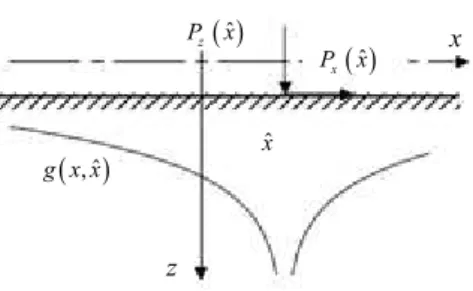
The solutions to the plane state problem for a homogeneous, linear elastic and isotropic substrate loaded by a concentrated force normal or tangential to the substrate boundary are known as Flamant’ and Cerruti’s solutions (Johnson, 1985; Kachanov et al., 2003), respectively. In particular, the surface displacement ui(x)
(with i = x, z) due to a point force P xi( )ˆ applied to the
substrate boundary may be expressed in closed form as
ui(x) = g x x( , )ˆ P xi( )ˆ (Fig. 2), where Green's function ˆ
( , )
g x x takes the following expression:
ˆ 2 ˆ ( , ) ln x x g x x E d − = − π (6)
DOI: 10.3844/sgamrsp.2018.30.45
Fig. 2: Green’s function g x x( , )ˆ related to point forces P xx( )ˆ , ˆ
( ) z
P x applied to the half-plane boundary
In Equation 6, E = Es or E = Es/(1− ν2s)for a generalized plane stress or plane strain state, respectively and d represents an arbitrary length related to a rigid-body displacement.
The displacements along x- and z-axes of a generic point of the substrate boundary due to tractions rx and rz
can be written as (Johnson, 1985; Kachanov et al., 2003):
( )
0 ˆ ˆ ˆ ( ) ( ) d ˆ ˆ ˆ ˆ ( ) d ( ) d 2 L x L x x x z z x x u x g x,x r x x c r x x r x x E = − − ∫
∫
∫
(7a)( )
0 ˆ ˆ ˆ ( ) ( ) d ˆ ˆ ˆ ˆ ( ) d ( ) d 2 L z L z x x x x x x u x g x,x r x x c r x x r x x E = + − ∫
∫
∫
(7b)where, x0, xL are the horizontal coordinates of the beam end
sections and c = 1-vs or c = (1-2vs)/(1-vs) for a generalized
plane stress or plane strain state, respectively.
Using the theorem of work and energy for exterior domains, it may be demonstrated that the total potential energy for the substrate, ∏soil, is given by (Tullini and Tralli,
2010; Tullini et al., 2012): soil ( ) d 2 L x x z z b r u r u x Π = −
∫
+ (8)Then, substituting Equation 7a and 7b into Equation 8 yields Πsoil = Πsoil,a + Πsoil,b, where:
( )
{
0 soil, ( ) d ˆ ( ) dˆ ˆ 2 ˆ ˆ ˆ ˆ ( ) d ( ) d 2 L a L x L x x x z z x x b r x x g x,x r x x c r x x r x x E Π = − − − ∫
∫
∫
∫
(9a)( )
{
0 soil, ( ) d ˆ ( ) dˆ ˆ 2 ˆ ˆ ˆ ˆ ( ) d ( ) d 2 L b L z L z x x x x x x b r x x g x,x r x x c r x x r x x E Π = − + − ∫
∫
∫
∫
(9b)Total Potential Energy for the Foundation-Substrate
System
Using Equation (5) and (9) leads to express the total potential energy for the beam-substrate system as:
, , , ,
beam a beam b soil a soil b
= + + +
∏ ∏
∏
∏
∏
(10)which is a mixed formulation with variational functions represented by displacements ubx,0, uz and rotation ϕ, as
well as interfacial shear and normal tractions rx and rz
along the beam-substrate interface. The use of Green's function (6) restricts the domain of integration to the foundation beam length.
Several particular cases derive from Equation 10. For example, in the case of a Timoshenko beam in frictionless contact with the soil, shear traction rx
vanishes and Equation 10 add space reduces to:
(
)
( )
beam d ˆ ˆ ˆ ( ) d ( ) d 2 L z z z z z L L U b p r u m x b r x x g x,x r x x Π = − − + ϕ −∫
∫
∫
(11)Finite Element Model
Both the foundation and the soil boundary are discretized into FEs. Although the mesh of the soil boundary can in theory be independent of that of the foundation, the same discretization will be adopted in the following. The ith FE is characterized by initial and end coordinates xi and xi+1, length li = |xi+1-xi| and
dimensionless local coordinate ξ = x/li.
As usual in the displacement-based FEM, the unknown displacement functions may be described in terms of nodal quantities, collected by vectors uxi = [ux,i,
ux,i+1]T and qzi = [uz,i, φi, uz,i+1, φi+1]T, according with the
following relations:
( ) ( ) , [ ( ), ( )]T ( )
a xi b zi
uξ =N ξu vξ ϕ ξ =N ξq (12a, b)
where, vector Na(ξ) and matrix Nb(ξ) contain the
interpolating shape functions.
In this study, the shape functions collected by matrix
Na(ξ) = [Na,1, Na,2] are linear Lagrangian polynomials
Na,1 1-ξ and Na,2 = ξ, whereas matrix Nb(ξ) assembles the
“modified” Hermitian shape functions already adopted by Minghini et al. (2009; 2010; Tullini and Tralli, 2010; Tullini et al., 2013b).
The soil tractions for the ith element, instead, are approximated by the following expressions:
( ) [ ( )]T , ( ) [ ( )]T
x a xi z b zi
r ξ = ρ ξ r r ξ = ρ ξ r (13a, b)
where, rxi, rzi indicate shear and normal tractions,
respectively, at the node locations along the substrate
x z ( ),ˆ g x x ( )ˆ z P x ( )ˆ x P x ˆx
boundary and vectors ρa, ρb collect constant or linear
shape functions.
The substitution of Equation 12 and 13 into the total potential energy (Equation 10), assemblage over all elements and request of stationarity for the functional, yield the following system of governing equations:
T = − q f K H r 0 H G (14) where: , , a xx b xz zz = = K 0 H 0 K H 0 K H H (15a, b) xx xz zx zz = G G G G G (15c) , , x x x z z z = = = u r f q r f q r f (16a, b, c)
It is worth noting that Equation 14 represents the discrete system of equations that govern the static behaviour of the beam-substrate system. In the previous expressions, Ka, Kb are the beam stiffness matrices and
fx, fz are the external load vectors. In addition, the
components of matrices Hxx, Hzz, Hxz are
foundation-substrate coupling terms, whereas matrices Gxx, Gzz, Gxz,
Gzx depend on surface tractions and are fully populated
(Tezzon et al., 2015).
In this study, equal substrate shape functions are used, i.e., ρa = ρb = ρ, resulting in the two conditions Gxx = Gzz
and Gzx = - Gxz and in the symmetry of matrices Gxx and Gzz.
Vectors q and r can be obtained from the solution to Equation 14. In particular, the following expressions hold:
1 T
, ( soil)
−
= + =
r G H q K K q f (17a, b)
where, Ksoil = H G−1 HT is the stiffness matrix of the
substrate. It is simple to show that Ksoil is symmetric. In
fact, (Ksoil)T = (H G−1 HT)T = H G−T HT = H G−1 HT =
Ksoil, since matrix G is symmetric (Tezzon et al., 2015).
It is worth noting that the second row of Equation 14, containing the governing equation of the discrete Galerkin method for the system of Equations 7a and 7b, includes the beam rotations due to substrate tractions. In particular, the compatibility of rotations between foundation beam and substrate is imposed through the introduction of the following term into Equation 5b:
[
z z x / 2]
dL
b r u r h x
−
∫
+ ϕ (18)Following a different approach, Cheung and Nag (1968; Wang et al., 2005) substituted piecewise constant tractions into Equation 7a and 7b and directly used those equations to obtain horizontal and vertical displacements of the substrate boundary, respectively. Such an approach assumes the presence of a finite number of equally spaced links between the foundation beam and the substrate. These links are pinned in correspondence of the foundation and clamped to the soil surface and make therefore to lose the rotation continuity at the interface. In the resulting soil matrix, rows and columns of zeros must then be added corresponding to the nodal rotations.
It can also be of interest to underline that the validity of Equation 17a is independent of the existence of a foundation beam. Equation 17a, indeed, may be used to compute the soil surface tractions originating from the definition of a generic displacement field q at the substrate boundary.
For a structure connected to a foundation beam, Equation 14 can be partitioned as reported by Tullini and Tralli (2010; Tullini et al., 2012). In particular, denoting with q1 and q2 the vectors of nodal displacements
referred to the structure only and those shared between structure and foundation beam, respectively and with f1
and f2 the corresponding load vectors, Equation (14)
takes the form:
11 12 1 1 21 22 2 2 T = − K K 0 q f K K H q f 0 H G r 0 (19)
Prismatic Beam Subjected to Uniform Loads
Beam stiffness matrices Ka, Kb and external load
vectors fx, fz can be rewritten as:
0 3 , b , a a b b E A D L L = = K K% K K% (20a, b) , a=ba b=bb f f% f f% (20c, d) where: , , 1 1 1 , 1 1 2 1 x i a i a i i L p l l − = = − K% f% (21a, b) 2 2 3 , 3 2 12 6 12 6 (4 ) 6 (2 ) 12 6 (1 ) symm (4 ) i i i i i i i b i i i i i i l l l l l L l l l − − − + ϕ − ϕ = + ϕ + ϕ K% (22) 2 2 T , T [ 2, 12, 2, 12] (1 ) [1, 2, 1, 2] b i z i i i i i i i i i p l l l l m l l = − + + ϕ ϕ − ϕ f% (23)
DOI: 10.3844/sgamrsp.2018.30.45
where, coefficient φi = 12Db/(k G A lb b b i2)vanishes in the case the shear deformation is negligible. The assemblage of global stiffness matrices Ka, Kb and load vectors fa, fb
from the corresponding element matrices Kai, Kbi and
load vectors fai, fbi is as usual. However, with a penalty
approach it is possible to include constraint equations into functional ∏ (Tullini et al., 2013a; 2013b).
Prismatic Beam with Piecewise Constant Surface
Tractions
In the following, only piecewise constant functions are used to interpolate rx and rz, i.e., the shape functions
for the soil tractions are assumed to be ρa(ξ) = ρb(ξ) = 1.
This assumption leads to the expressions for matrices
(
)
,xx= zz= b E
G G G% Gxz=
(
bc E)
G%xz and H = bH% reported by Tezzon et al. (2015) in § 3.2.Making use of Equation 20 and Equation 14 may then be rewritten as follows:
3 T b D L b b b b E = − q K H f r H G 0 % % % % % (24) where: 2 0 a , xx b xz zz λ = = K 0 H 0 K H 0 K H H % % % % % % % (25a, b) T , xx xz x xz zz z c c = = G G f G f G G f % % % % % % % % (25c, d)
with λ0 = L/rg and the radius of gyration rg = h/ 12.
Therefore, solutions (17) reduce to:
-1 T = E r G H q% % (26a) 3 3 b soil D LK% +(αL)K% q= bf% (26b) being 1 T soil − =
K% H G H% % % the nondimensional stiffness matrix for the substrate and:
3 3
b
L b E L D
α = (27)
Parameter αL rules the response of the foundation-substrate system (Biot, 1937). Low values of αL characterize short beams stiffer than soil, whereas high values of αL correspond to slender beams on a relatively stiff soil.
Mesh sizes of beam and substrate boundary can be defined independently of one another and shape functions different than used to obtain Equation 14 may
be adopted as well. For example, Tullini et al. (2012) used quadratic Lagrangian bar elements including one or two equal substrate elements, whereas Tullini and Tralli (2010) used beam-substrate matrices obtained adopting four equal soil elements for each beam element.
Foundation Beam in Frictionless Contact with the
Substrate
For a beam resting in frictionless contact on an elastic half-plane, rx = fx = 0 and Equation 14 reduces to the
following expression: T z z b zz z zz zz = − q f K H r 0 H G (28)
In particular, the second row of Equation 28 contains the governing equation of the discrete Galerkin method for displacement uz(x) and relates beam rotations to
vertical reactions. Differently, Cheung and Zienkiewicz (1965) proposed a collocation method to uz(x), but in this
case no angular continuity between foundation beam and substrate is ensured. Accordingly, they appied a static condensation to beam matrix Kb, so as to cancel out rows
and columns corresponding to the nodal rotations.
Rigid Flat Punch with Piecewise Constant Surface
Tractions
With reference to the profile of a rigid flat indenter, the prescribed displacements are:
, ,
( ) , ( ) , ( )
x x o z z o o o
u x =u u x =u − ϕ x ϕ x = ϕ (29a, b, c)
where, ux,o, uz,o and ϕo are specified at the origin x = z =
0. Therefore, vector qo = [ux,o, uz,o, ϕo]T, collecting the
displacements prescribed at the origin, governs the displacement field generated by a rigid flat punch. Thus, substituting Equation 13 into variational principle (10), in which terms ∏beam,a and ∏beam,b are obtained from
Equation 5a and 5b for strain energies
Ubeam,a = Ubeam,b = 0, assembling over all substrate
elements and requiring the potential energy to be stationary, the following system of equations is obtained:
T o o o o = − q f 0 H r 0 H G (30) Where: T , , T , , T , , o xx x o o o zz o z o o z o P P M φ = = h 0 H 0 h f 0 h (31a, b)
Vector fo collects the three external load resultants: , , , x o L x z o L z P =
∫
p d x P =∫
p d x (32a, b) ( ) o L z M =∫
m−p x d x (32c)where, as vectors ho,xx, ho,zz, ho,ϕz, in the case ρa,i = ρb,i =
1, takes the following expressions:
1 , , , , , , , . 2 i i o xx i o zz i i o z i i x x h h bl hφ bl + + = = = − (33a, b)
With regard to the FE discretization, coordinate xj of the
generic jth node of the mesh is assumed to be given by:
xp 1 2 1 if 0 /2 2 if /2 e el el el j n j el el j j n n x x n j n β − − ≤ ≤ = − < ≤ (34)
with nel being the total number of FEs in the mesh and
βexp the so-called grading exponent (Graham and
McLean 2006). A uniform mesh is obtained by assuming βexp = 1.
Plane Strain Linear Elastic Analysis of a RC
Single-Cell Culvert on Elastic Substrate
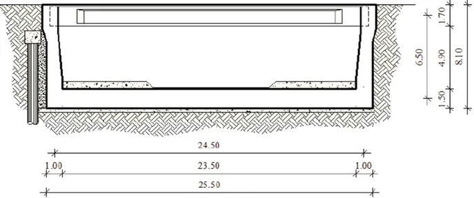
The present example is aimed at assessing the soil-structure interaction for the realistic case of a box culvert (Fig. 3), that is a very common structural typology usually made of reinforced concrete. The
choice of size, shape and number of cells in a culvert plays a fundamental role to control the water flow, especially during extreme weather events such as major floods and washouts and influences then significantly management and maintenance costs of infrastructures.
The foundation slab of the culvert, showing thickness h = 1.5 m and the two 1-m thick abutments are cast-in-place members (Fig. 3). The abutments support precast I-beams mutually connected at the top through a 0.2 m-thick cast-in-place slab. The resulting ribbed slab has an overall depth of 1.7 m and is simply-supported at the ends.
The generic culvert cross-section is reduced to a plane frame (Fig. 4) having out-of-plane dimension b = 1 m, column height H = 6.5 m and beam span length
L = 24.5 m.
Locking-free Timoshenko beam elements with a shear correction factor kb = 5/6 are used to develop the
numerical model of the culvert. In particular, the foundation (beam F in Fig. 4a) in perfect adhesion with the substrate is modelled using a uniform mesh of nel = 512 Timoshenko beam FEs. According to the
present formulation, these elements have the centreline at a distance from the substrate boundary equal to a half of the foundation thickness. A series of preliminary tests confirmed that the numerical model ensures convergent solutions.
With regard to the top beam (B3 in Fig. 4a), bending moment releases are introduced in correspondence of the nodes in common with columns B1 and B2 to reproduce the hinged connections between ribbed slab and abutments (Fig. 4).
Fig. 3: Cross-section of the RC single-cell culvert investigated in plane strain conditions, with the foundation slab in perfect adhesion with the soil and the top slab simply-supported on the abutments
DOI: 10.3844/sgamrsp.2018.30.45
Fig. 4: Plane frame corresponding to the box culvert shown in Fig. 3, with B1 and B2, B3 and F indicating the two columns (abutments), the upper beam (top slab) and the foundation, respectively. The two load cases investigated are: (a) self-weight
and (b) horizontal load px uniformly distributed along beam B3
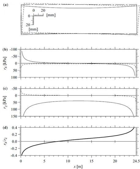
Fig. 5: Frame analysis results: (a) deflections of the frame subjected to self-weight (solid line) and lateral load (dashed line) acting separately; corresponding (b) horizontal (rx) and (c) vertical (rz) soil reactions; and (d) ratio rx/rz for the two load cases acting
simultaneously. Dash-dot line in (a) represents the undeformed frame
A plane strain analysis is conducted by assuming Young's modulus Es = 30 MPa and Poisson's ratio
vs = 0.3 for the soil substrate and Eb/ (1− ν2b) = 30 GPa for all RC elements. The stiffness parameter for the foundation-soil system results to be αL = 3.8.
The two load cases shown in Fig. 4 are considered, i.e., the self-weight, represented in Fig. 4a by uniform distributions of vertical loads and a horizontal load px
uniformly distributed along beam B3 (Fig. 4b). This load can be regarded as an earthquake action equal to about 20% of the structural self-weight.
Figure 5a illustrates with solid and dashed lines the deformed configurations of the culvert under self-weight and earthquake loads, respectively, acting not combined with one another, whereas the dash-dot line represents the undeformed configuration. The maximum vertical
displacement under gravity loads, equal to about 10 mm, is observed at the top beam midspan. The maximum lateral displacement due to the horizontal load is approximately 7 mm.
Tangential and normal reactions underneath the foundationare reported in Fig. 5b and 5c, respectively, for the two load cases. The maximum reactions are obtained at the ends of the foundation beam and the reactions for the frame subjected to self-weight are always larger than for the lateral load case. With regard to traction rx, only two small portions of the substrate
boundary near the ends are active (Fig. 5c).
Finally, ratio rx/rz obtained when vertical and lateral
loads are applied simultaneously is reported in Fig. 5d. For a typical sandy soil with angle of internal friction φs = 25 deg, parameter µsf = rx/rz = tan[(2/3)rs] = 0.3 may
be viewed as the foundation-soil friction coefficient (Bowles, 1997). Wherever this friction coefficient is exceeded, the displacement continuity between soil and foundation at the substrate boundary is lost and the perfect adhesion hypothesis must be released. In the present example, with the exception of two 4 m long regions in proximity of the end sections, ratio rx/rz varies
almost linearly taking values not greater than 0.2. Values of rx/rz greater than 0.3 are attained only in two very
narrow portions of the foundation in correspondence on the connections with the abutments.
Plastic Hinge Modeling
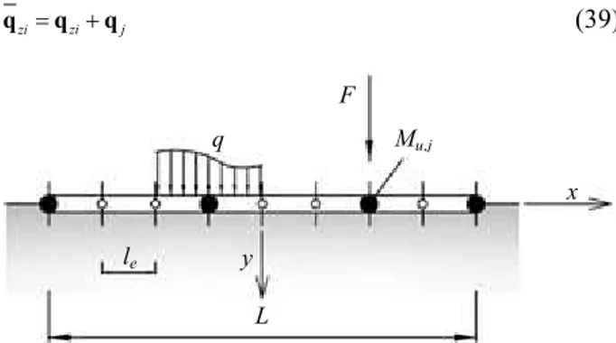
In this Section, material nonlinearity will be introduced into the mixed formulation proposed above. Altough the general case of a shear flexible foundation in perfect adhesion with the half-plane could in theory be considered, Euler-Bernoulli foundations in frictionless contact with the substrate will be assumed for example purposes. Under this assumption, a generic, ith beam element is characterized by the following equilibrium equation (Equation 28):
i= bi zi− zi+ zzi zi
n K q f H r (35)
where, subscript i indicates quantities related to the generic finite element. In particular, qzi = {v1i, φ1i, v2i,
φ2i}T is the vector of nodal degrees of freedom,
collecting vertical displacements vki and rotations φki,
with k = 1, 2 indicating first and second element nodes. Vector ni = {V1i, M1i, V2i, M2i}T collects nodal forces
applied to the element, namely shear forces Vki and
bending moments Mki, whereas Hzzi rzi represents the
vector of equivalent nodal forces generated by the uniform traction underneath the beam element.
A beam characterized by FEs with a flexural plastic hinge at one or both ends (Fig. 6) is now considered (Baraldi, 2013). The plastic hinge is modeled as a semi-rigid connection (Hasan et al., 2002). Hence, a bending
moment-rotation relationship (M-θ), where θ represents the post-elastic rotation, is introduced to describe the stiffness degradation of the beam cross-section following the formation of the plastic hinge. In particular, the rotational stiffness of a semi-rigid connection at the kth node (Chen and Lui, 2005) is substituted by the post-elastic bending stiffness Rk = dMk/dθk of the
cross-section (Hasan et al., 2002). Moreover, the simple procedure proposed by Shakourzadeh et al. (1999) is adopted for taking account of the plastic hinge M-θ relation. Consequently, considering a beam FE with flexural plastic hinges located at the end nodes only and introducing the vector of post-elastic nodal displacements qj = {w1, θ1, w2, θ2}T, the joint constitutive
relation may be written in the form:
i= j j
n K q (36)
Joint stiffness matrix Kj is defined as follows:
1 2
{ , , , }
j=diag ∞R ∞R
K (37)
where, R1 and R2 are the flexural plastic hinge stiffnesses
at the beam ends, whereas assuming infinite stiffnesses related to shear forces means that no post-elastic vertical joint displacements w1, w2 are allowed.
The equilibrium of a generic beam element resting on an elastic half-plane reported in Equation 35 is replaced by the relation:
bi zi zzi i= zi− + zi
n K q f H r (38)
where, Kbi is the modified stiffness matrix of the element, zi
f is the modified equivalent load vector and
{
1, 1, 2, 2}
T
i i
i i
zi= v ϕ v ϕ
q is the vector of equivalent nodal displacements that may be splitted as follows by separating elastic displacements and post-elastic rotations:
zi j
zi= +
q q q (39)
Fig. 6: Foundation beam on elastic half-plane subdivided into equal FEs, with potential plastic hinges (solid circles) at the ends and along its length
F Mu,j q le y L x
DOI: 10.3844/sgamrsp.2018.30.45
Substituting qzi=qzi−qj into Equation 35 and remembering Equation 36, the modified matrices and load vector in Equation 38 become:
, ,
bi= bi zi= zi zzi= zzi
K CK f Cf H CH (40a, b, c)
where, correction matrix C (Shakourzadeh et al., 1999; Minghini et al., 2009; 2010) depends on the stiffness matrix of the element and on the plastic hinge stiffnesses collected in Kj:
(
)
1(
1)
1 j j bi bi j − − − = + = + C K K K I K K (41)Note that matrix Hzzi is modified in the same way as stiffness matrix Kbi and equivalent load vector fzi, see Equation 40a-c. Finally, matrices Kb and Hzz and equivalent load vector fz of the entire fondation are generated by assembling local matrices as usual. Classical Newton-Raphson procedure is used to carry out the incremental-load analysis.
In the following, rectangular cross-sections are considered and, for simplicity, a rigid-perfectly plastic model is adopted. Thus, ultimate moment Mu,k and ultimate
rotation θu,k completely characterize the plastic hinge
behavior at the kth node. Furthermore, the post-elastic bending stiffness assumes the value Rk = ∞ when the
section is in the elastic range (Rk = 109Db in the following
numerical examples, in order to avoid numerical instabilities) and Rk = 0 (Rk = 10−6Db in the following) when
the corresponding bending moment reaches Mu,k.
It is worth noting that if the beam end sections are both in the elastic range, matrix C reduces to the identity matrix I and no changes are made to element matrices and load vector. Conversely, if the beam ends are both in the plastic range, matrix C has null elements in correspondence of the post-elastic nodal rotation and the vector of nodal forces reduces to ne = {V1, Mu,1, V2, M u,2}T
ni = {V1i, Mu,1i, V2i, Mu,2i}T.
Standard third-order Hermitian polynomials will be used to approximate beam vertical displacements, whereas soil tractions will be interpolated by means of piecewise constant functions.
Plane Strain Nonlinear Analysis of a RC Box
Culvert on Elastic Substrate
A RC pipe on elastic half-plane is studied taking material nonlinearity into account by placing potential plastic hinges where large bending moment values are expected. The structure consists of a pipe or concrete box-culvert 22.10 m long, built to grant the free flow of a stream under a railway line (Mancini, 2010). The cross-section dimensions are reported in Fig. 7. Plane strain
conditions are considered. Consequently, a pipe segment of unit length is assumed. The top slab is covered by a soil bed with thickness of 2.5 m and a ballast with thickness of 0.8 m, yielding the uniformly distributed loads referred to as qsoil and qballast, respectively (Fig. 7). Lateral abutments
are obviously subject to the earth pressure (Fig. 7), linearly varying from qtop to qbottom. Furthermore, a service
load due to a train qtrain acts on the upper beam and causes
a pressure pearth on the left column. The values of the loads
represented in Fig. 7 are collected in Table 1.
The pipe is made of concrete of class C 25/30, reinforced with steel bars with nominal yield strength fy
= 500 MPa; the corresponding design properties are computed in accordance with Eurocode 2 (CEN, 2004). Mancini (2010) adopted a Winkler support with a vertical reaction modulus c = 20 N/cm3. Adopting Biot's (1937) relation between modulus c and the elastic properties of the corresponding half-plane:
1/3 1/3 4 4 4 4 4 /3 0.710 0.282 2 s s b b E b E b c D D = = (42)
the soil under the structure turns out to have the parameters of a soft clay, characterized by Es = 16 MPa
and weight per unit volume γS = 19 kN/m3. The
corresponding soil-structure interaction parameter αL for the pipe foundation is equal to 1.55.
Structural elements were designed by Mancini (2010) adopting Eurocode 2 design rules. Figure 8 shows the actual reinforcements adopted. Each section is characterized by a nominal concrete cover of 35 mm. An ultimate moment Mu(N), depending on local axial load
N, is defined for each cross-section where a potential
plastic hinge is located.
Beam-column connections are modeled as infinitely rigid links having length equal to one half of the corresponding cross-section height; then, the remaining parts of columns and top beam are discretized by 4 equal beam FEs, whereas the foundation beam is discretized by 8 equal beam FEs (Fig. 8). Potential plastic hinges are placed at the FE ends near beam-column connections, at foundation midpoint and at top beam and column midpoint, where maximum bending moment values are expected. Assuming a local Cartesian coordinate system for each element having x axis directed from left to right for the foundation and top beam FEs and directed upward for the column FEs, Table 2 reports beam FE ends having a potential plastic hinge. Each plastic hinge is characterized by a N-Mu diagram, which provides the
ultimate bending moment of the section as a function of axial load. Horizontal displacements are prevented at the foundation level by fixing end 1 of element #17.
In the following, incremental analyses of the pipe subjected to various loads are carried out taking account of material nonlinearity. A rigid-perfectly plastic moment-rotation relationship is adopted as plastic hinge constitutive law. The behaviour of plastic hinge sections is monitored by N-M curves, which are compared with the corresponding N-Mu diagrams depending on section
geometry and steel reinforcements adopted. Each incremental analysis is stopped when a local or global collapse mechanism is achieved. Then, the computed ultimate load is compared with an upper bound represented by the limit load corresponding to the collapse mechanism of a portal with fixed column bases.
Table 1: Values of distributed loads applide to the pipe shown in Fig. Parameter Value [kN/m] qsoil 47.5 qballast 14.4 qtrain 74.5 qtop 30.95 qbottom 93.65 pearth 20
Table 2: Potential plastic hinge positions for the FE model of the pipe
FE # Node 1 Node 2
2, 6, 12, 14, 18, 20, 24, 26 Yes −
5, 9, 13, 15, 19, 21, 25, 27 − Yes
Fig. 7: Pipe cross-section (dimensions in meters) and applied loads
DOI: 10.3844/sgamrsp.2018.30.45
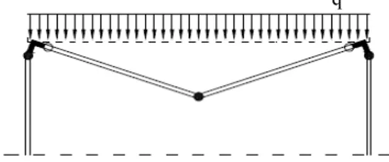
The first example is characterized by an increasing load
q on the top beam of the pipe (Fig. 9). The vertical
displacement at top beam midpoint, d, is taken as a reference parameter to determine the load-deflection (q-d) curve. The first plastic hinge is formed at top beam midpoint (end 2 of element #13, end 1 of element #14). The second and third plastic hinges are formed at column tops (end 2 of elements #21 and #27). Then, a collapse mechanism for the top beam is obtained (Fig. 10). The ultimate load of the structure is qu,1 = 513 kN/m, which is
quite close (96%) to the limit load that may be determined for a portal frame with clamped column bases and with the same collapse mechanism (qlim,1 = 536 kN/m). The first
plastic hinge formation is characterized by q = 386 kN/m and d = 0.0094 m, whereas the second and third ones are formed with q = 513 kN/m and d = 0.0175 m (Fig. 11).
The second example takes account of the self-weight of the pipe and considers again an increasing distributed load q on the top beam (Fig. 12). In this case, at equal incremental load q, the self-weight makes the axial force in the column elements increase with respect to the previous example. Then, ultimate loads may be quite different. However, similarly to the previous example, a local collapse mechanism for the top beam is obtained (Fig. 10). The ultimate load of the structure is qu,2 = 359
kN/m, which is 32% smaller than the limit load that may be determined for a portal frame with clamped column bases and with the same collapse mechanism (qlim,2 = 528
kN/m). In this case, for q = 0, displacement at top beam midpoint is nonzero due to the effect of the self-weight (Fig. 13). The first plastic hinge is formed for q = 234 kN/m and d = 0.012 m. The second and third plastic hinge are formed for q = 359 kN/m and d = 0.027 m.
For the purpose of comparison, a third example is prentented, already reported by Baraldi and Tullini (2017). An increasing distributed load λqtrain on the top
beam and the corresponding increasing lateral load
λpearth along the left column are considered, with all
other loads remaining constant. Vertical displacement d at top beam midpoint (element #13, end 2 and element #14, end 1) is assumed as reference and λ-d curve is presented in Fig. 14. For λ = 0, the displacement at top beam midpoint is d = 0.013 m due to the effect of dead loads and soil pressures.
The first plastic hinge is formed at the top of the right column (element #27, end 2) with λ = 3.18 and d = 0.077 m (triangle in Fig. 14). However, after the formation of this plastic hinge, the slope of the load-displacement curve does not change significantly. The second plastic hinge is localised at the top beam midpoint (element #13, end 2 and element #14, end 1) with λ = 3.45 and d = 0.082 m (solid circle in Fig. 14). After the formation of the second plastic hinge, the slope of load-deflection curve is quite lower than before. The third and fourth plastic hinges develop, almost at the same load increment, at foundation midpoint and at the top of the left column.
Fig. 9: Pipe loaded by an incremental vertical force q uniformly distributed along the top beam
Fig. 10: Collapse mechanism for the top beam
Fig. 11: Load-deflection plot for the pipe loaded by an incremental vertical force q distributed along the top beam
Fig. 12: Pipe loaded by self-weight and by an incremental vertical force q uniformly distributed along the top beam
600 400 200 0 0 0.025 q [k N/ m ] d[m] 536 513 q q Lp L q Lp L
Fig. 13: Load-deflection plot for the pipe loaded by self-weight and incremental vertical force q distributed along the top beam
Fig. 14: Load-deflection curve obtained from the analysis of the pipe under dead loads and increasing service loads
Fig. 15: Pipe deformation during incremental analysis
Then, a collapse mechanism for the top beam is obtained. Due to the plastic hinges at the top of the columns and at top slab midpoint, indeed, three aligned plastic hinges are obtained. Correspondingly, the ultimate load multiplier is λu = 3.99, with d = 0.102 m (symbol × in Fig. 14). Some
of the deformed shapes of the pipe during the incremental analysis are depicted in Fig. 15.
(a)
(b)
Fig. 16: N-M values experienced under incremental loads by cross-sections where plastic hinge formation is
attained, compared with the relevant N-Mu diagrams:
stress resultants for end section 2 of finite elements (a) #5 and (b) #13 corresponding to midpoints of foundation and top beams, respectively
-3 -2 -1 0 1 2 3 4
5 4 3 2 1 0 3 2 1 0 -1 -2 -3 -20 -15 -10 -5 0 5 N[N] M [N m ] ×106 el. 13, end 2 ×106 ×106 3 2 1 0 -1 -2 -3 -20 -15 -10 -5 0 5 el. 5, end 2 ×10⁶ M [N m ] ×106 N[N]
DOI: 10.3844/sgamrsp.2018.30.45
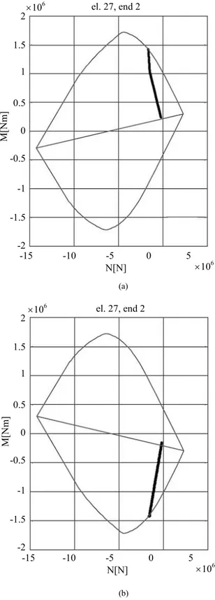
(a)
(b)
Fig. 17: N-M values experienced under incremental loads by cross-sections where plastic hinge formation is
attained, compared with the relevant N-Mu
diagrams: stress resultants for end section 2 of finite elements (a) #21 and (b) #27 corresponding to the top of the columns
Figures 16 and 17 show the bending moment variation as a function of the axial force for the potential plastic hinge sections activated by the incremental analysis. Axial forces turn out to be very small for the plastic hinge sections at the foundation and top beam midpoints (Figs. 16a and 16b), whereas plastic hinge sections at the top of the columns (Figs. 17a and 17b) are characterized by increasing compressive forces. Moreover, a slope variation in the N-M curve due to first and second plastic hinge development is clearly shown in Fig. 17a for the last plastic hinge section.
An upper bound for the ultimate load may be obtained considering a portal frame with fixed column bases. The corresponding collapse mechanism, having three aligned plastic hinges along the top slab, yields a load multiplier λlim = 5.70, which is larger than λu
because actual soft soil support and non-symmetric deformed shape of the entire pipe are neglected.
Conclusion
A coupled Finite Element-Boundary Integral Equation (FE-BIE) model for the analysis of prismatic beams and frames perfectly bonded to a homogeneous, linearly elastic and isotropic two-dimensional half-space is presented. The model relies upon the combination of the displacement-based FEM with an integral equation defined at the substrate boundary (BIE). The foundation structure is discretized into standard FEs. At the same time, a Green’s function is used into equations that relate tangential and normal displacements of the soil surface with surface tractions (Equation (7a, 7b)). Under the plane state hypothesis, the theorem of work and energy for exterior domains is used to develop a mixed variational formulation, in which the independent variables are nodal beam displacements and rotations and nodal soil tractions. To take the influence of the shear deformation into account, the foundation is described using Timoshenko beam elements.
Extensive convergence rate tests demonstrated the noteworthy efficiency of the present formulation. For example, for an Euler-Bernoulli foundation beam with
L/h = 10 and αL = 20 loaded by a vertical point force at
midspan, the exponent of convergence rate Cneq-λ, with
neq being the number of equations, is 1.99 for the present
model, 1.02 for the formulation proposed by Cheung and Nag (1968) and lies between 0.98 and 1.02 for very accurate FE models using bidimensional, four-node finite elements (Tezzon et al., 2015).
The formulation is then extended to the case of material nonlinearity. To this purpose, the efficient procedure proposed by Hasan et al. (2002) for pushover analysis of framed structures is modified by adopting the semi-rigid joint model proposed by Shakourzadeh et al. (1999). The resulting procedure allows to account for structural nonlinear behavior by placing potential plastic 2 1.5 1 0.5 0 -0.5 -1 -1.5 -2 -15 -10 -5 0 5 M [N m ] N[N] ×106 ×106 el. 27, end 2 2 1.5 1 0.5 0 -0.5 -1 -1.5 -2 -15 -10 -5 0 5 N[N] ×106 M [N m ] el. 27, end 2 ×10⁶
hinges into the discrete model of the structure without adding further elements and degrees of freedom. For simplicity, a rigid-perfectly-plastic relation is adopted to describe the moment-rotation relationship of plastic hinges and ultimate bending moments are evaluated by assuming structural members made of RC.
The proposed model is initially applied to the soil-structure interaction analysis for a linear elastic RC box culvert. Assuming a state of plane strain, the culvert cross-section is identified with a frame subjected to self-weight and a uniformly distributed lateral load. The loads are transferred to the soil by means of a shear flexible foundation beam in perfect adhesion with the substrate boundary. The foundation beam is discretized by means of a uniform mesh of 512 FEs. The proposed formulation is shown to be effective in the evaluation of frame deflections and soil reactions.
Finally, the formulation is applied to the incremental-load analysis of a pipe with rectangular cross-section in frictionless contact with an elastic half-plane. The numerical examples show the effectiveness of the model in reproducing the damage evolution from the first plastic hinge formation up to the achievement of a collapse mechanism.
Further developments of this research will be dedicated to the extension of the proposed model to the three-dimensional case.
Acknowledgement
The present investigation was developed in the framework of the Research Program FAR 2017 of the University of Ferrara. This paper was presented at the 6th International Workshop on Design in Civil and Environmental Engineering held at the University of Cagliari during November 9-10-11, 2017.
Author’s Contributions
All authors contributed equally to the research work presented in this paper.
Ethics
The corresponding author confirms that all other authors have read and approved the manuscript and no ethical issue arose. All sources of information were properly referenced.
References
Baraldi, D., 2013. Nonlinear analysis of structures on elastic half-space by a FE-BIE approach. PhD Thesis, University of Ferrara.
Baraldi, D. and N. Tullini, 2017. Incremental analysis of elastoplastic beams and frames resting on an elastic half-plane. J. Eng. Mechan.
Bielak, J. and E. Stephan, 1983. A modified Galerkin procedure for bending of beams on elastic foundations. SIAM J. Sci. Stat. Comput., 4: 340-352.
DOI: 10.1137/0904028
Biot, M.A., 1937. Bending of an infinite beam on an elastic foundation. J. Applied Mechan. Trans., 4: A1-A7. Bowles, E.J., 1997. Foundation Analysis and Design. 1st
Edn., McGraw-Hill, London, UK.
CEN, 2004. Design of concrete structures, Part 1-1: General rules and rules for buildings (Eurocode 2), Brussels. Eur. Committee Standardization.
Chen, W.F. and E.M. Lui, 2005. Handbook of Structural Engineering. 2nd Edn., CRC Press, Boca Raton, Florida.
Cheung, Y.K. and D.K. Nag, 1968. Plates and beams on elastic foundations–linear and non-linear behaviour. Geotechnique, 18: 250-260.
DOI: 10.1680/geot.1968.18.2.250
Cheung, Y.K. and O.C. Zienkiewicz, 1965. Plates and tanks on elastic foundations – an application of finite element method. Int. J. Solids Struc., 1: 451-461. DOI: 10.1016/0020-7683(65)90008-9
Giberson, M.F., 1969. Two nonlinear beams with definition of ductility. J. Struct. Divis. ASCE, 95: 137-157.
Graham, I.G. and W. McLean, 2006. Anisotropic mesh refinement: The conditioning of Galerkin boundary element matrices and simple preconditioners. SIAM J. Numer. Anal., 44: 1487-1513.
DOI: 10.1137/040621247
Hasan, R., L. Xu and D.E. Grierson, 2002. Push-over analysis for performance-based seismic design. Comput. Struct., 80: 2483-2493.
DOI: 10.1016/S0045-7949(02)00212-2
Johnson, K.L., 1985. Contact Mechanics. 1st Edn., Cambridge University Press, Cambridge, UK. Kachanov, M., B. Shafiro and I. Tsukrov, 2003. Handbook
of Elasticity Solutions. 1st Edn., Academic Publishers, Dordrecht, The Netherlands, Kluwer.
Kikuchi, N., 1980. Beam bending problems on a Pasternak foundation using reciprocal variational-inequalities. Quart. Applied Math., 38: 91-108. DOI: 10.1090/qam/575834
Mancini, G., 2010. Design of Members. Linear Members. In: Structural Concrete Volume 1: Textbook on Behaviour, Design and Performance: Design and Performance: Design of Concrete Structures, Conceptual Design, Materials. FFIDB (Ed.), Fib Fédération Internationale Du Béton, Lausanne,ISBN-10: 2883940916, pp: 37-60. Minghini, F., N. Tullini and F. Laudiero, 2009. Elastic
buckling analysis of pultruded FRP portal frames having semi-rigid connections. Eng. Struc., 31: 292-299. DOI: 10.1016/j.engstruct.2008.09.003
DOI: 10.3844/sgamrsp.2018.30.45
Minghini, F., N. Tullini and F. Laudiero, 2010. Vibration analysis of pultruded FRP frames with semi-rigid connections. Eng. Struc., 32: 3344-3354.
DOI: 10.1016/j.engstruct.2010.07.008
Ribeiro, D.B. and J.B. Paiva, 2015. An alternative BE– FE formulation for a raft resting on a finite soil layer. Eng. Anal. Boundary Elements, 50: 352-359. DOI: 10.1016/j.enganabound.2014.09.016
Selvadurai, A.P.S., 1979. Elastic Analysis of Soil-Foundation Interaction. 1st Edn., Elsevier Scientific Publishing Company, Amsterdam, New York, ISBN-10: 0444416633, pp: 543.
Shakourzadeh, H., Y.Q. Guo and J.L. Batoz, 1999. Modeling of connections in the analyses of thin-walled space frames. Comput. Struct., 71: 423-433. DOI: 10.1016/S0045-7949(98)00241-7
Tezzon, E., N. Tullini and F. Minghini, 2015. Static analysis of shear flexible beams and frames in adhesive contact with an isotropic elastic half-plane using a coupled FE-BIE model. Eng. Struct., 104: 32-50. DOI: 10.1016/j.engstruct.2015.09.017
Tullini, N. and A. Tralli, 2010. Static analysis of Timoshenko beam resting on elastic half-plane based on the coupling of locking-free finite elements and boundary integral. Computat. Mechan., 45: 211-225. DOI: 10.1007/s00466-009-0431-2
Tullini, N., A. Tralli and D. Baraldi 2013a. Stability of slender beams and frames resting on 2D elastic half-space. Arch. Applied Mechan., 83: 467-482. DOI: 10.1007/s00419-012-0694-5
Tullini, N., A. Tralli and D. Baraldi, 2013b. Buckling of Timoshenko beams in frictionless contact with an elastic half-plane. J. Eng. Mechan., 139: 824-831. DOI: 10.1061/(ASCE)EM.1943-7889.0000529 Tullini, N., A. Tralli and L. Lanzoni, 2012. Interfacial
shear stress analysis of bar and thin film bonded to 2D elastic substrate using a coupled FE-BIE method. Finite Elements Anal. Design, 55: 42-51. DOI: 10.1016/j.finel.2012.02.006
Wang, Y.H., L.G. Tham and Y.K. Cheung, 2005. Beams and plates on elastic foundations: A review. Progress Struc. Eng. Mater., 7: 174-182.