NUMERICAL SIMULATION
OF FLUID-STRUCTURE INTERACTION PHENOMENA
Facoltà di Ingegneria
Dipartimento di Ingegneria Civile, Edile e Ambientale
Dottorato in Ingegneria Idraulica (XXXI ciclo)
Candidato: Luca Barsi
Matricola: 793557
2 INDEX
Summary………...….4
Chapter 1 - Introduction………..6
Chapter 2 - The model……….……..….18
2.1 Integral form of the Navier-Stokes equations over a moving control volume………..……..19
2.2 Integral form of the URANS equations over a moving control volume……….22
2.3 The structural motion equations……….………….28
2.4 Implicit pressure correction methods………..…………29
2.5 The numerical model used in this work……….…….35
Chapter 3 - Test case 1: slender body with rectangular cross-section………...……43
3.1. Geometry and numerical modelling………..……….43
3.2. Static validation……… …….44
3.3. Dynamic simulations……….………….45
Chapter 4 - Test case 2: Forth Road Bridge deck………...……….49
4.1. Geometry and numerical modelling………...…50
4.2. Initial conditions for the stability analysis………...50
4.3 Dynamic validation……….52
Chapter 5 - Aeroelastic stability study of the Forth Road Bridge deck………...…..58
5.1 Coupled flutter type characterisation……….….58
5.2 Coupled flutter onset mechanism………...….60
5.3 Post-critical flutter mechanism………...………64
3 Conclusions………..87 References………..……..91
4
Summary
In this thesis, a new method for the investigation of aeroelastic phenomena for long-span bridges is proposed: the aerodynamic fields and the motion of structure are simulated simultaneously and in a coupled manner. The structure is represented as a bidimensional elastically suspended rigid body with two degrees of freedom whose natural frequencies correspond to those of the fundamental flexural and torsional modes of vibration of the structure. The aerodynamic fields are simulated by numerically integrating the Unsteady Reynolds-Averaged Navier-Stokes (URANS) equations with a finite volume scheme on moving grids which adapt to the structural motion. The URANS equations are completed by the turbulent closure relations which are expressed as a function of the turbulent kinetic
energy, the turbulence frequency and the strain tensor according to the k- SST approach.
The presented model is used in order to identify the critical flutter wind velocity of the Forth Road Bridge deck, and the numerical results are compared with those of an experimental campaign. For wind velocities equal or greater than the critical wind flutter velocity, the deck starts to oscillate increasingly. It is demonstrated that the reason for the onset of the torsional-branch coupled flutter lies in the fact that, within each of the first oscillation cycles, there is a portion of the cycle in which the energy supplied by the aerodynamic field to the deck motion is more than the energy extracted in the rest of the cycle. Then it is shown that the reason for
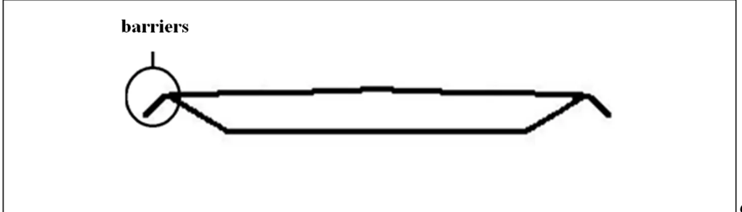
5 the amplification of the instability resides in the drifting of large vortical formations along the deck surface. The numerical model is also used to test the effect, on the aeroelastic stability of the Forth Road Bridge deck, of the introduction of a couple of sloping barriers at the windward and leeward bridge deck edges. It is demonstrated that the aerodynamic modifications produced by the introduction of such barriers is effective in increasing the critical flutter velocity and mitigating the vibration amplitudes which develop during the flutter instability.
6
Chapter 1
Introduction
Long span bridges are susceptible to an oscillatory unstable aero-elastic phenomenon, named flutter, in which the bridge deck motion acquires a divergent character and the oscillation amplitudes grow rapidly to the point of causing the structural failure (Dowell, 2014). Bridge decks with bluff cross-sections are generally prone to the torsional flutter phenomenon: the case of the Tacoma Narrows Bridge deck is a well known example. Bridge decks with streamlined cross-sections are generally prone to the coupled (torsional-flexural) flutter phenomenon: the possibility that the latter kind of instability takes place is relevant in the case in which the bridge deck has torsional and flexural natural modes of oscillation closely spaced at low natural frequencies (Frandsen, 2004). Matsumoto et al. (2010) carried out analytical investigations on the mechanisms of coupled flutter. These authors distinguish two different types of coupled flutter. The first type is the torsional branch (TB) coupled flutter, which is dominated by a fundamentally torsional vibration and in which the vertical oscillations have small amplitudes. The second type is the heaving-branch (HB) coupled flutter, which is dominated by a fundamentally heaving vibration accompanied by torsional oscillations with small amplitudes.
7 Traditionally the critical flutter wind velocity of long span bridge decks is identified through the Scanlan approach (Nieto et al., 2014). A first central element of said approach lies in representing the structure as a bidimensional rigid body with two degrees of freedom, having mass per unit length and mass moment of inertia per unit length equal to those of the deck. In the above-mentioned schematisation the rigid body is considered as attached to an elastic vertical spring and to an elastic torsional spring whose stiffnesses are calibrated in order to give the natural frequencies corresponding to the fundamental flexural and torsional modes of vibration of the structure. Astiz (1998) highlights that schematising the structure as a bidimensional rigid body with two degrees of freedom supposes that there is full coherence between the shapes of the flexural and torsional modes of vibration along the span. The main criticism moved to the previous approach comes from Katsuchi et al. (1999). These authors underline that, in some cases, the possibility has been highlighted that in the coupled flutter not only the fundamental flexural and torsional modes of vibration participate in the instability: the latter authors notice that, in the coupled flutter, further modes of vibration can overlap the fundamental modes of vibration, giving rise to aeroelastic instability conditions characterized by more complex flutter mode shapes.
The original method proposed in this thesis is based on the need to overcome the limit of the Scanlan traditional approach, which substantially consists in using the above fundamental free modes of vibration and, starting from these modes, performing stability
8 analyses. Actually, also an elementary oscillator can oscillate not only with the fundamental vibration modes but also with other vibration modes, as a consequence of the load to which it is subjected. Consequently, a stability analysis which is able to overcome the above limitation must necessarily simulate the aerodynamic field and the structural motion in a coupled manner, given the fact that they interact each other.
A second central element of the above-mentioned Scanlan approach lies in modelling the aerodynamic forces as linear functions of the structural displacements, under the assumption of purely sinusoidal motions. This linear dependance is expressed via some appropriate coefficients, called flutter derivatives. The most widely used method for the evaluation of flutter derivatives is based on the following fundamental passages. The aerodynamic fields developing around a bridge deck cross-section (that is made to oscillate according to a predefined sinusoidal law of motion) are simulated. The time history of the forces produced by the aerodynamic fields on the bridge deck surface is approximated by a sinusoidal function. Consequently, the forces produced by the aerodynamic fields on the bridge deck are assumed to be linearly dependent on the structural displacements. From the above-mentioned linear dependence the flutter derivative calculation is performed.
Many authors (Larsen and Walther, 1998; Mendes and Branco, 1998; Taylor and Vezza, 2002; Morgenthal and McRobie, 2002; Vairo, 2003; Sarwar et al., 2008) propose models for the flutter derivatives estimation and use them in order to identify the critical flutter wind
9 velocity of the bridge decks.. Astiz (1998) and Dowell (2014) highlight that the linear relation between the forces produced by the aerodynamic field on the deck and the structural displacements (formulated in the Scanlan approach) proves to be acceptable only in the event that the amplitude of structural oscillations is limited. Furthermore, the same authors underline that the above-mentioned linear relation does not make it possible to take into account the effects of the unsteady vortical structures developed in the fluid-structure interaction. In this thesis (as said above), the aerodynamic fields and the motion of structure are simulated simultaneously and in a coupled manner. According to this approach, the pressure and velocity fluid fields, that develop around the structure at every instant, are simulated; starting from the aerodynamic pressures, the lift force and the twisting moment, acting on the structure at every instant, are computed; once the above-mentioned aerodynamic forces are known, the structural displacements are calculated; these displacements, in turn, modify the computational domain and the boundary for numerical integration of the fluid motion equations and, as a consequence, modify the structure of the aerodynamic fields. Thereby the limitation represented by the hypothesis of linear dependence of the aerodynamic forces from the structural displacements, which is a central element in the flutter derivatives approach, is exceeded. The simultaneous and coupled simulation of the aerodynamic fields and the structural motion allows the identification of the critical flutter wind velocity in a direct way. Furthermore, the approach based on the coupled and simultaneous simulation of
10 the aerodynamic fields and the structural motion proves to be more effective than that based on the flutter derivatives especially in cases where the fluid-structure interaction gives rise to the formation of large vortices which, produced at the leading edge, move towards the trailing edge and amplify the oscillations of the structure itself.
The latter methodology presents excessively high computational costs when applied to the three-dimensional simulation of the multimodal coupled flutter. However, Starossek (1998) underlines that schematizing the structure as a bidimensional system with two degrees of freedom makes it possible to favourably predict the critical flutter wind velocity when the modal shapes associated with the fundamental flexural and torsional modes of vibration do not greatly differ along the span-wise direction; in the latter case, the above-mentioned modes of vibration are able to couple and form a common flutter mode shape. In this context, as in the bimodal Scanlan approach, the structure can be represented as a bidimensional elastically suspended rigid body with two degrees of freedom whose natural frequencies correspond to those of the fundamental flexural and torsional modes of vibration of the structure. Braun and Awruch (2008) underline that the hypothesis of rigid body is acceptable when the elastic deformations of the deck cross-section can be considered small compared with the vertical and torsional displacements of the same deck cross-section.
The simulation of the aerodynamic fields can be performed by finite volume techniques on unstructured grids (Gallerano and Napoli, 1999; Oka and Ishihara, 2009) or on
boundary-11 conforming curvilinear grids (Gallerano and Cannata, 2011, Rossmanith et al., 2004). The continuity and momentum balance equations admit the velocity components and pressure as dependent variables. In the case of incompressible fluids, the pressure calculation can be performed by adopting explicit methods of fractional step type, or implicit methods of pressure-correction type. The first method is based on the calculation of a predictor velocity field from the momentum balance equation in which the term related to the pressure gradient is omitted: this field is not solenoidal but admits the same curl as that of the velocity field at the successive instant. A corrector irrotational field exists whose divergence is equal to those of the predictor field, but with opposite sign. This term is explicited in terms of a scalar function gradient. The laplacian of the scalar function equalized to the divergence (with negative sign) of the predictor velocity field allows the calculation of the above scalar function; from this function, the calculation of the corrector field can be performed and, consequently, also the calculation of the velocity field at the successive instant. The second method consists of gaining, from the velocity and pressure field at the instant t, the velocity
and pressure field at the instant t+t by means of the so-called outer iterations and inner
iteration. A predictor velocity field is calculated at the outer iteration implicitly (by means of an inner iteration process), where the pressure gradient is assumed to be equal to that of the previous iteration. The predictor velocity field is introduced into the equation of the laplacian of the pressure, from the solution of which the pressure value is obtained. This pressure value
12 is in turn introduced in the momentum balance equation, thus providing the velocity field at the end of the m-th outer iteration. The outer iteration process ends when the velocity and
pressure field at the instant t+t satisfies both the continuity equation and the momentum
balance equation.
.As said above, the instabilities of the decks are related to the unsteady phenomena of the aerodynamic fields (Larsen, 2000; Sarwar and Ishihara, 2010; Mannini et al., 2014), and in particular to the formation of unsteady vortex structures. In the literature, the most complete simulation of the turbulent flow fields is performed through the Large Eddy Simulation (LES) by applying a spatial filter to the fluid velocity fields and simulating all the vortex structures whose dimensions are equal or greater than those of the spatial filter. Bosch and Rodi (1998) highlight that at high Reynolds numbers, the stochastic turbulent fluctuations are superimposed on the periodic unsteady motion of the vortex structures. These authors proposed the simulation of the flow field characterized by the above-mentioned unsteady vortex structures by decomposing the instantaneous flow quantities in a time mean component, in a periodic component and in a turbulent fluctuating component. Following this approach, the sum of the time mean and the periodic part gives rise to the ensemble-averaged component of the flow quantities. The latter are calculated by the numerical integration of the ensemble-averaged continuity and momentum equations; the complete spectrum of the stochastic motion is simulated by a statistical turbulence model. The models coherent with the
13 above-mentioned approach are named in the literature as Unsteady Reynolds-Averaged Navier-Stokes (URANS) models. It must be highlighted that the URANS approach provides a more simplified representation of the aerodynamic field compared to the Large Eddy Simulation (LES) approach. On the other hand, the URANS methodology has relatively low computational costs. Furthermore, the URANS approach makes it possible (even though less rigorously than the LES approach) to simulate the quasi-periodic unsteady vortex structures of the aerodynamic field (Mannini et al., 2010) and (with reference to aeroelastic instability phenomena such as vortex induced vibrations and flutter) to well identify the onset velocities and the amplitudes of the induced structural oscillations.
The fluid velocity field around an object is always three-dimensional since (as has been said) is characterised by high vorticity, flow separation and unsteady vortex structures (Mannini et al., 2011). The bidimensional simulations are not able to adequately represent the energy transfer from the larger vortical structures to the smaller vortical structures, as this transfer is related to the vortex stretching (which is three-dimensional). However, Frandsen (2004) stresses that the effects of the aerodynamic field in the span-wise direction of the deck can be neglected in cases where the deck cross-section has sharp edges. Furthermore, many authors (Bruno and Khris, 2003; Mannini et al., 2010; Mannini et al., 2010b; Shimada and Ishihara, 2011) highlight that the aerodynamic field around the bridge decks show relevant quasi-periodic vortical structures characterised by the direction of the vorticity vector parallel
14 with the span-wise direction: the quasi-periodic vortical structures, characterised by the direction of the vorticity vector parallel to the transverse direction, are negligible in the opinion of the above-mentioned authors. In the above-mentioned conditions, bidimensional simulation schemes can produce acceptable results from an engineering point of view.
The above-mentioned authors follow the line indicated by Bosch and Rodi and simulate the aerodynamic instabilities by using a two-dimensional URANS model in which the fluid motion equations are completed by two turbulence statistical equation models. In the models proposed by the above-mentioned authors the span-wise diffusion processes are taken into account by a conveniently calibrated eddy viscosity introduced in the turbulent closure relations. The turbulent closure relations for the fluid motion equations are expressed as a function of the transport equations of turbulent kinetic energy k and the rate of viscous
dissipation , or as a function of the transport equations of the turbulent kinetic energy and the
turbulence frequency . Brusiani et al. (2013) argue that the k- model has to be preferred to
the k- model for the simulation of the fluid dynamic fields near the wall: the k- model does
not allow the direct integration through the boundary layer and over-estimates the turbulent
kinetic energy in stagnation regions near the wall, while the k- model allows the direct
integration through the boundary layer and improves the wall boundary layer unsteady solution, but is highly sensitive to the inlet turbulent boundary condition. Menter (2009)
15 proposed the k- Shear Stress Transport (SST) model, which consists of a blending between
the k- model and k- model and preserves the main advantages of the k- model.
In this thesis, a new method for the investigation of aeroelastic phenomena for long-span bridges is proposed: the aerodynamic fields and the motion of structure are simulated simultaneously and in a coupled manner. The structure is represented as a bidimensional elastically suspended rigid body with two degrees of freedom whose natural frequencies correspond to those of the fundamental flexural and torsional modes of vibration of the structure. The Unsteady Reynolds Averaged Navier-Stokes (URANS) equations are solved on block-structured moving grids and are defined in integral form starting from the three-dimensional Leibniz rule and the substantial derivative of the material volume integral of the momentum. The solution procedure of the momentum balance equation in implicit form is of pressure-correction type. The finite-volume method of collocated type implies the reconstruction of the velocity and pressure values in the calculation cells which, in this thesis, uses the Rhie-Chow procedure.
The model has been validated by comparing the numerical results with the experimental ones related to a slender body with rectangular cross-section and the Forth-Road Bridge deck. The model validation is performed both in static conditions (i.e. under the assumption that all the degrees of freedom of the body are restrained) and dynamic conditions (i.e. under the
16 assumption that the body is free to oscillate in the bending degree of freedom and in the torsional degree of freedom). In the static case, the Strouhal number, the lift and drag coefficients are taken as benchmark parameters by comparing the numerical results with those obtained experimentally with regard to the case study of the slender body with rectangular cross-section. In the dynamic case, the comparison is performed in terms of critical flutter wind velocity by comparing the numerical results with those obtained experimentally with regard to the case study of the Forth Road Bridge deck.
A deep insight into the analysis and the detailed representation of the different phenomena that produce the onset of flutter for long span bridge decks with streamlined cross-section is proposed. Such detailed representation makes it possible to deduce that the reason for the coupled flutter onset lies in the fact that, within each of the first oscillation cycles, there is a portion of the cycle in which the energy supplied by the aerodynamic field to the deck motion is more than the energy extracted in the rest of the cycle. Moreover, the same detailed representation allows one to deduce that the reason for the amplification of the aeroelastic instability is ascribable to the formation and drift of large vortical formations along the surface of the deck. The numerical model is also used to test the effect, on the aeroelastic stability of the deck, of the introduction of a couple of sloping barriers at the windward and leeward bridge deck edges. It is demonstrated that the aerodynamic modifications, produced by the introduction of such barriers, is effective in increasing the
17 critical flutter velocity and mitigating the vibration amplitudes which develop during the flutter instability.
18
Chapter 2
The model
In this chapter, the model utilized in order to perform the numerical investigation of the bridge flutter phenomenon is described. The chapter is organized as follows:
in paragraph 2.1, the procedure is presented by which the integral form of the Navier-Stokes equations over a moving control volume is deduced;
starting from the integral form of the Navier-Stokes equations over a moving control volume, in paragraph 2.2 the procedure is then presented by which the integral form of the Unsteady-Averaged Navier-Stokes (URANS) equations, which are numerically solved in this work, is deduced;
in paragraph 2.3, the structural motion equations used in the present work are presented;
in paragraph 2.4, a general overview on the implicit pressure correction methods is provided;
in paragraph 2.5, the finite volume method is shown by which the URANS equations adopted in this work are solved.
19 2.1 Integral form of the Navier-Stokes equations over a moving control volume
In this paragraph, the Navier-Stokes equations are defined in integral form starting from the three-dimensional Leibniz rule and the substantial derivative of the material volume integral of the momentum.
Let ρ and u⃗ be, respectively, the density and the fluid velocity vector. Let ∆V (τ) be a time-varying control volume bounded by a surface, of area ∆A (τ), every point of which moves with a velocity that is different from the fluid velocity. By using the three dimensional Leibniz integral rule, the time derivative of the integral of ρu⃗ over the volume ∆V (τ) can be expressed as
∫∆ ( ) ⃗ = ∫∆ ( ) ⃗ + ∫∆ ( ) ⃗( ⃗ ∙ ⃗) (1)
in which n⃗ is the outward unit vector normal to the surface of area ∆A (τ) and v⃗ is the velocity vector with which the points belonging to the surface of area ∆A (τ) move.
Let us consider a material fluid volume, i.e. a time-varying volume which moves with the fluid and always encloses the same fluid particles. Let ∆V(τ) be a time-varying material volume and that is delimited by a surface of area ∆A(τ) every point of which moves with the same velocity of the fluid. It is known that the time derivative of the integral of ρu⃗ over the
20
∫∆ ( ) ⃗ = ∫∆ ( ) ⃗ + ∫∆ ( ) ⃗( ⃗ ∙ ⃗) (2)
in which the velocity vector with which the points belonging to the surface of area ∆A(τ) coincides with the fluid velocity vector u⃗. It is assumed that at instant τ, ∆V (τ) =
∆V(τ). By replacing the first term on the right hand side of Eq. 2 by the term ∫∆ ( ) ⃗dV extracted from the right hand side of Eq. 1, Eq. 2 becomes
∫∆ ( ) ⃗ = ∫∆ ( ) ⃗ + ∫∆ ( ) ⃗( ⃗ − ⃗) ∙ ⃗ (3)
The left hand side of Eq. 3 represents the expression of the time derivative of the integral of ρu⃗ over a material volume (material derivative), which is valid in the case of a control volume whose boundary surface points move with a velocity, v⃗, that is different from the fluid velocity, u⃗. By equating the rate of change of the momentum of a material volume, expressed by the right hand side of Eq. 3, to the total net force in this direction (Newton’s law), we obtain the integral form of the momentum equation over a moving control volume
∫∆ ( ) ⃗ + ∫∆ ( ) ⃗( ⃗ − ⃗) ∙ ⃗ = ∫∆ ( ) ⃗ + ∫∆ ( ) ∙ ⃗ (4)
in which is the stress tensor. From Eq. 4, it is possible to deduce that, for an
incompressible fluid, the integral form of the momentum equation over a moving control volume reads
21 ∫∆ ( ) ⃗ + ∫∆ ( ) ⃗( ⃗ − ⃗) ∙ ⃗ = ∫∆ ( ) ⃗ + ∫∆ ( ) ∙ ⃗ (5)
in which
= − ̅ + 2 ̅ (6)
where is the dynamic viscosity, ̅ is the rate of strain tensor and ̅ is the identity matrix. By introducing Eq. 6 into Eq. 5 and using the divergence theorem, Eq. 5 can be rewritten as
∫∆ ( ) ⃗ + ∫∆ ( ) ⃗( ⃗ − ⃗) ∙ ⃗ = ∫∆ ( ) ⃗ − ∫∆ ( )∇
+ ∫∆ ( )2 ̅ ∙ ⃗ (7)
in which is the dynamic fluid viscosity and ∇= .
By adopting the same control volume, ∆ ( ), the expression of the time derivative of the integral of ρ over the material fluid volume reads
∫∆ ( ) = ∫∆ ( ) + ∫∆ ( ) ( ⃗ − ⃗) ∙ ⃗ (8)
From Eq. 8 it is possible to deduce that, for an incompressible fluid, the integral form of the continuity equation over a moving control volume reads
22 Bearing in mind that ∆A(τ) is the area of the surface delimiting the time-varying control volume ∆V(τ) that at instant τ coincides with the material volume, also the following relation holds valid for an incompressible fluid
∫∆ ( ) ⃗ ∙ ⃗ = 0 (10)
Following the same logical procedure already indicated for the definition of Eq. 3, if we assume that, at instant τ, ∆V (τ) = ∆V(τ) and introduce Eq. 10 into Eq. 9, we obtain
∫∆ ( ) + ∫∆ ( ) ⃗ ∙ ⃗ = 0 (11)
which is known in literature as the so-called Geometric Conservation Law (GCL, see Hertel et al., 2013).
2.2 Integral form of the URANS equations over a moving control volume
Bosch and Rodi (1998) highlight that at high Reynolds numbers, the stochastic turbulent fluctuations are superimposed on the periodic unsteady motion of the vortex structures. These authors proposed the simulation of the flow field characterized by the above-mentioned unsteady vortex structures by decomposing the instantaneous flow quantities in a time mean component, in a periodic component and in a turbulent fluctuating component. Following this approach, the sum of the time mean and the periodic part gives rise to the ensemble-averaged
23 component of the flow quantities. The latter are calculated by the numerical integration of the ensemble-averaged continuity and momentum equations; the complete spectrum of the stochastic motion is simulated by a statistical turbulence model. The models coherent with the above-mentioned approach are named in the literature as Unsteady Reynolds-Averaged Navier-Stokes (URANS) models.
Following this approach, the instantaneous values of the fluid velocity ⃗( ) and the
fluid pressure ( ) are decomposed in the time mean components ⃗ and ̅, the periodic
components ⃗( ) and ( ), and the fluctuating components ⃗ and
⃗( ) = ⃗ + ⃗( ) + ⃗ (12)
( ) = ̅ + ( ) + (13)
The sum of the time mean and the periodic part are defined as the ensemble averaged component 〈⃗( )〉 and 〈 ( )〉, which are resolved in the numerical calculation. Eqs. (12), (13)
become respectively
⃗( ) = 〈 ⃗( )〉 + ⃗ (14)
( ) = 〈 ( )〉 + (15)
For an incompressible fluid, by neglecting the viscous term the integral form of the ensemble averaged continuity and momentum equations over a moving control volume read
24
∫∆ ( ) + ∫∆ ( )(〈 ⃗〉 − ⃗) ∙ ⃗ = 0 (16)
∫∆ ( )〈 ⃗〉 + ∫∆ ( )〈 ⃗〉(〈 ⃗〉 − ⃗) ∙ ⃗ = ∫∆ ( ) ⃗ − ∫∆ ( )∇〈 〉
+ ∫∆ ( ) ∙ ⃗ (17)
in which is the Reynolds stress tensor, which is defined as
= −〈 ⃗ ⨂ ⃗ 〉 (18)
where ⨂ is the tensor product operator. The unknown term 〈 ⃗ ⨂ ⃗ 〉 is related to the
ensemble averaged strain rate tensor 〈 ̅〉 and the ensemble averaged turbulent kinetic energy per unit mass 〈 〉 through the relation
〈 ⃗ ⨂ ⃗ 〉 = −2 〈 ̅〉 + 〈 〉 ̅ (19)
where t is the kinematic eddy viscosity.
The turbulent closure relations for the fluid motion equations can be expressed as a function of the transport equations of turbulent kinetic energy k and the rate of viscous
dissipation , or as a function of the transport equations of the turbulent kinetic energy and the
turbulence frequency . Brusiani et al. (2013) argue that the k- model has to be preferred to
the k- model for the simulation of the fluid dynamic fields near the wall: the k- model does
25 kinetic energy in stagnation regions near the wall, while the k- model allows the direct
integration through the boundary layer and improves the wall boundary layer unsteady solution, but is highly sensitive to the inlet turbulent boundary condition. Menter (2009)
proposed the k- Shear Stress Transport (SST) model, which consists of a blending between
the k- model and k- model and preserves the main advantages of the k- model. In this
work, the turbulent closure relations are completed by the k- SST model. In integral form,
the integral form of the k and w equations over a moving control volume read
∫ 〈 〉 ∆ ( ) + ∫∆ ( )〈 〉(〈 ⃗〉 − ⃗) ∙ ⃗ = ∫ − ∗〈 〉〈 〉 ∆ ( ) + ∫∆ ( )∇ ∙ [( + )∇〈 〉] (20) ∫ 〈 〉 ∆ ( ) + ∫∆ ( )〈 〉(〈 ⃗〉 − ⃗) ∙ ⃗ = ∫∆ ( ) − 〈 〉 + ∫∆ ( )∇ ∙ [( + )∇〈 〉] + ∫ 2(1 − ) 〈 〉∇〈 〉 ∙ ∇〈 〉 ∆ ( ) (21)
in which ‹› is the ensemble averaged turbulence frequency and
= 〈 〉
( 〈 〉, ) (22)
= 2〈 〉〈 〉 (23)
26 = 〈 〉 〈 〉+ 〈 〉 (25) = ℎ ∗〈 〉 〈 〉 , 〈 〉 , 〈 〉 (26) = ℎ ∗ 〈 〉 〈 〉 , 〈 〉 (27) = 2 〈 〉 〈 〉 〈 〉 , 10 (28)
where y is the distance to the nearest wall, S is the invariant measure of the strain rate,
F1 and F2 are blending functions. All constants are computed as = 1F1 + 2(1-F1). The
constants for this model are: * = 0.09, 1 = 5/9, 1 = 3/40, k1 = 0.85, 1 = 0.5, 2 = 0.44,
2 = 0.0828, k2 = 1, 2 = 0.856.
With respect to the turbulence modelling of the near-wall region, two different approaches are usually adopted. The first one is the Low-Reynolds Number (LRN) approach, which uses a refined mesh close to wall in order to resolve all the important physics. The second one is the High-Reynolds Number (HRN) approach, which bridge the near-wall region by using the wall functions. In this work, at the solid walls the near-wall treatment proposed by Menter et al. (2003) is used. Such approach consists in automatically switching from a
LRN approach to a HRN approach as the grid is coarsened. The k- SST model has the
27 logarithmic region. However, the analytical expression of is not known in the buffer region.
Therefore this method consists in blending the wall value of between the viscous sub layer
and the logarithmic region. A blending function depending on y+ is used (y+ = (y u / where
y is the distance from the wall and u is the friction velocity). The solutions for in the
viscous sub layer and the logarithmic region are respectively
=
. ; = . (29)
where is the Von Karman constant. They are reformulated in terms of y+ and the following smooth blending is performed:
( ) = ( ) + ( ) (30)
A similar formulation is used for the velocity profile near the wall
= ; =
( ) (31)
where U1 is the velocity of the first calculation cell and
= ( ) + ( ) (32)
This formulation gives the relation between the velocity near the wall and the wall shear stress. For the k-equation, a zero flux boundary is applied, as this is correct for both the low-Re and the logarithmic limit. The zero gradient boundary condition has been imposed at the
28 outlet for all the fluid dynamic quantities (fluid velocity, turbulent kinetic energy, turbulence frequency).
2.3 The structural motion equations
The motion of the body can be described in terms of three displacement components,
, where and are respectively the translational displacement component in the
horizontal direction x (positive from left to right) and the translational displacement
component in the vertical direction y (positive upwards), and denotes the rotational
displacement component (positive nose-up). The governing equation for the body motion is
̈ + ̇ + = (33)
where M, C and K are respectively the mass matrix, the damping matrix and the
stiffness matrix; X is a vector which lists the displacement components ; F is a vector
which lists the component fx in the x direction of the force exerted by the aerodynamic field
on the body, the component fy in the y direction of the above-mentioned force and the twisting
moment m generated by the above-mentioned force on the body. The components fx, fy and
the twisting moment m are calculated by integrating the pressures, the viscous stresses and
the turbulent stresses over the surface of the structure.
29
̈ + ̇ + = ( , ̇, ̈, , ̇ , ̈) (34)
̈ + ̇ + = ( , ̇ , ̈ , , ̇, ̈) (35)
where m and I are respectively the mass and the mass moment of inertia per unit length
of the deck; cy and c are respectively the structural damping coefficients in the vertical and
torsional degree of freedom; ky and k are respectively the stiffness constant of the vertical
elastic spring and the stiffness constant of the torsional elastic spring, and and are
respectively the vertical displacement of the centre of gravity of the body and the rotational
angle of the body around the shear centre. The stiffness ky and k are calibrated in order to
give the natural frequencies corresponding to the fundamental flexural and torsional natural modes of vibration of the structure. The damping coefficients are calculated according to the formulation proposed in the work by Hines et al. (2009) on the basis of the given damping ratios.
2.4 Implicit pressure correction methods
The continuity and momentum balance equations admit the velocity components and pressure as dependent variables. In the case of incompressible fluids, the pressure calculation can be performed by adopting explicit methods of fractional step type, or implicit methods of pressure-correction type. The first method is based on the calculation of a predictor velocity
30 field from the momentum balance equation in which the term related to the pressure gradient is omitted: this field is not solenoidal but admits the same curl as that of the velocity field at the successive instant. A corrector irrotational field exists whose divergence is equal to those of the predictor field, but with opposite sign. This term is explicited in terms of a scalar function gradient. The laplacian of the scalar function equalized to the divergence (with negative sign) of the predictor velocity field allows the calculation of the above scalar function; from this function, the calculation of the corrector field can be performed and, consequently, also the calculation of the velocity field at the successive instant. The second method consists of gaining, from the velocity and pressure field at the instant t, the velocity
and pressure field at the instant t+t by means of the so-called outer iterations and inner
iteration. A predictor velocity field is calculated at the outer iteration implicitly (by means of an inner iteration process), where the pressure gradient is assumed to be equal to that of the previous iteration. The predictor velocity field is introduced into the equation of the laplacian of the pressure, from the solution of which the pressure value is obtained. This pressure value is in turn introduced in the momentum balance equation, thus providing the velocity field at the end of the m-th outer iteration. The outer iteration process ends when the velocity and
pressure field at the instant t+t satisfies both the continuity equation and the momentum
31 adopted for the solution of the momentum balance equation in implicit form, in the following a general overview on the implicit pressure correction methods is provided.
In general, if an implicit method is used to advance the fluid velocity in time, the discretized form of the momentum equation at the new time step + 1 may be written as
⃗ + ∑ ⃗ = ⃗ − (∇ ) (36)
where is the index of the arbitrary velocity node and is the index of the generic
neighbor node. Eq. 36 cannot be solved directly as the coefficients (and possibly the source
term ⃗) depend on the unknown solution ⃗ . It follows that Eq. 36 must be solved
iteratively.
With regards to the simulation of an unsteady flow, two different levels of iterations exist within one time step. The first level refers to the so-called outer iterations, which are those iterations at the end of which the coefficients and the source term of the momentum equation are updated. The second level refers to the so-called inner iterations, which are those iterations that are performed on the momentum equation in which the coefficients and the source term are computed on the basis of the velocity and pressure field obtained at the previous outer iteration. On each outer iteration , the following equation is solved by successive inner iterations
32 in which the last term on the right hand side is computed on the basis of pressure field obtained at the end of the previous outer iteration. It is easy to deduce that the velocity field ⃗ ∗ obtained by solving Eq. 37 does not normally satisfy the continuity equation. It follows that ⃗ ∗ cannot represent the estimate of the solution ⃗ at the end of the current outer
iteration; instead, it is a predictor velocity field (which is the reason for it carries an asterisk) and need to be corrected in order that the continuity equation is satisfied.
The predicted velocity value at node , which has been obtained by solving Eq. 37, can be formally expressed by using the following relation
⃗ ∗ = ⃗ − (∇ ) (38)
in which
⃗ = ⃗ − ∑ ⃗ ∗ (39)
A better estimate of ⃗ at the end of the current iteration would be given by
⃗ = ⃗ − (∇ ) (40)
in which the pressure gradient (∇ ) is unknown. To follow, the procedure is shown by which the pressure gradient (∇ ) to introduce into Eq. 40 is calculated: bearing in mind that, for an incompressible flow, the discretized form of the continuity condition at the new time
33
∑ ⃗ ∙ ⃗ = 0 (41)
we enforce the continuity condition by inserting the value of ⃗ into Eq. 41. According
to the momentum interpolation method, if a collocated grid is used this velocity value can be expressed by mimicking Eq. 40 as follows
⃗ = ⃗ − (∇ ) (42)
where ⃗ and can be calculated by interpolating ⃗ , ⃗ and ,
respectively. By inserting Eq. 42 into Eq. 41, we obtain the so-called discretized Poisson pressure equation
∑ ⃗ ∙ ⃗ = ∑ (∇ ) ∙ ⃗ (43)
Once Eq. 43 has been solved, the pressure gradient (∇ ) can be computed and used into Eq. 40 to correct the velocity value at node . We then have, at the end of the current
outer iteration, a velocity field which satisfies the continuity equation (and hence is called
corrector velocity field), but both the velocity and pressure fields do not satisfy Eq. 36. We
then begin another outer iteration, and the process is continued until a velocity field which satisfies both the momentum equation and the continuity equation is obtained.
34 Synthetically, with regards to the simulation of an unsteady incompressible flow on a collocated grid, the numerical procedure consists of the following passages:
1. based on the velocity field obtained at the previous outer iteration, calculate the
coefficients , and the source term ⃗ ; furthermore, based on the pressure field obtained at the previous outer iteration, calculate the pressure term (∇ ) ;
2. solve Eq. 37 iteratively (inner iterations), thus obtaining ⃗ ∗, ⃗ ∗;
3. calculate ⃗ , ⃗ from Eq. 39;
4. calculate ⃗ and by interpolating ⃗ , ⃗ and ,
respectively;
5. solve Eq. 43 iteratively (inner iterations), thus obtaining the pressure field at the current outer iteration ;
6. calculate ⃗ , ⃗ from Eq. 40;
7. if the velocity field ⃗ satisfies the momentum equation, go to the next time
35 2.5 The numerical model used in this work
In this paragraph, the finite volume method is shown by which Eqs. 10, 11 and 17 equations used in this work are solved. In order to make the text easier to follow, in the following the ensemble averaged quantities are not enclosed by brackets 〈 〉.
2.5.1 Discretisation of the momentum equation
The discretised form of Eq. 17 is
⃗ ⃗ ⃗
∆ + ∑ ⃗ ∙ ⃗ − ̇ ⃗
= ∑ , ⃗ ∙ (∇ ⃗) − (∇ ) (44)
where the three-level second-order accurate backward scheme is used for temporal discretization (Ferziger and Peric, 2012). In Eq. 44, the subscript and indicate the
cell-centre and the face-cell-centre values of the generic fluid quantity, while + 1, and − 1
indicate the new time instant and the two previous time instant.
The face-centre velocity ⃗ in the convective term of Eq. 44 is calculated by using the
so-called Gamma interpolation scheme (Jasak et al., 1999). When this scheme reduces to a linear interpolation of the neighbouring cell-centre values, the face-centre velocity results by the relation
36
⃗ = ⃗ + (1 − ) ⃗ (45)
in which = .
The face normal derivative of velocity ⃗ ∙ (∇ ⃗) in the diffusive term is calculated
as follows
⃗ ∙ (∇ ⃗) = ∆⃗ ⃗ ⃗ ⃗ + ⃗ − ∆⃗ ∙ (∇ ⃗) (46)
in which the second term at the right-hand side is used to take into account the non-orthogonality of the mesh (Jasak, 1996).
By inserting Eqs. 45, 46 into Eq. 44, one obtains
⃗ ⃗ ⃗
∆ + ∑ ⃗ ∙ ⃗ − ̇ [ ⃗ + (1 − ) ⃗ ]
= ∑ , ∆⃗ ⃗ ⃗ ⃗ + ⃗ − ∆⃗ ∙ (∇ ⃗) − (∇ )
(47)
By dividing Eq. 47 for and by posing
= ∑ ⃗ ∙ ⃗ − ̇ + , ∆⃗⃗ +
37
⃗ = ∑ , ⃗ − ∆⃗ ∙ (∇ ⃗) +
∆ ⃗ − ∆ ⃗
(49)
Eq. 47 can be rewritten as
⃗ + ∑ ⃗ = ⃗ − (∇ ) (50)
2.5.2 Derivation of the discretised pressure equation
The discretised form of Eq. 10 is
∑ ⃗ ∙ ⃗ = 0 (51)
From Eq. 50 we have
⃗ = ⃗ ∑ ⃗ − (∇ ) (52)
By posing
⃗ = ⃗ − ∑ ⃗ (53)
Eq. 52 can be rewritten as
38 According to the momentum interpolation method (Norris, 2000), the cell-face velocity ⃗ in Eq. 51 can be expressed by mimicking Eq. 54 as follows
⃗ = ⃗ − (∇ ) (55)
where ⃗ and can be calculated by linearly interpolating ⃗ , ⃗ and ,
respectively (Rhie and Chow, 1983).
By inserting Eq. 55 into Eq. 51, the discrete pressure equation for the cell is obtained
∑ ⃗ ∙ (∇ ) = ∑ ⃗ ∙ ⃗ (56)
2.5.3 Calculation of the cell-face volume fluxes
The discretised form of Eq. 11 is
∆ − ∑ ̇ = 0 (57)
where the three-level second-order accurate backward scheme is used for temporal discretisation.
The difference between the cell volumes at consecutive time levels , + 1 can be calculated as
39
− = ∑ (58)
Analogously, the difference between the cell volumes at consecutive time levels − 1,
can be calculated as
− = ∑ (59)
It’s easy to verify that, by simple passages, the following relations can be derived from Eqs. 58, 59
3 − 4 + = ∑ 3 − (60)
By inserting Eq. 60 into Eq. 57, we obtain
∆ ∑ 3 − = ∑ ̇ (61)
from which it derives that, if the cell-face volume fluxes are calculated by means of the following expression
̇ =
∆ − ∆ (62)
40
2.5.4 Numerical calculation procedure
1. Calculate global lift force and twisting moment acting on the structure at the current time step.
2. Once the global face acting on the structure at the current time step are known, solve the equations governing the motion of the 2DOF system.
3. Once the displacements of the 2DOF system at the current time step are known, calculate the displacements of the mesh nodes belonging to the structure.
4. Together with the position of the boundary mesh nodes (which are fixed), the updated position of the mesh nodes belonging to the structure acts as a boundary condition for the mesh motion problem, whose solution provides the displacements of the interior mesh nodes. In this work, the mesh motion problem has been solved by using a mesh movement algorithm based on using Inverse Distance Weighting (see Uyttersprot, 2014).
5. Once the whole mesh is updated, calculate the cell-face volume fluxes using the expression
̇ =
∆ − ∆ (63)
6. Start the outer iteration loop in order to calculate the velocity and pressure filed at the current time step:
41 (i) solve the discretised momentum equation
⃗ ∗+ ∑ ⃗ ∗ = ⃗ − (∇ ) (64)
in which the coefficients , and the source term ⃗ are explicitly computed from the velocity field obtained at the end of the previous outer iteration and the cell-face volume fluxes obtained at step 6, and the pressure gradient (∇ ) is computed form the pressure field obtained at the end of the previous outer iteration;
(ii) solve the discretised pressure equation
∑ ⃗ ∙ ⃗ = ∑ (∇ ) ∙ ⃗ (65)
in which the coefficients ⃗ , are computed by linearly interpolating the
corresponding coefficients ⃗ , ⃗ and , respectively, and the coefficients ⃗ , ⃗ are
computed from the velocity field obtained at step (i);
(iii) calculate the corrected velocity field by using the relation
⃗ = ⃗ − (∇ ) (66)
and update the cell-face values ⃗ ∙ ⃗ which appear in the convective term by
42
⃗ ∙ ⃗ = ⃗ ∙ ⃗ − ⃗ ∙ (∇ ) (67)
in which the pressure gradient (∇ ) is computed from the pressure field obtained at step (ii);
(iv) if the velocity field obtained at step (iii) satisfies the momentum equation, go to step 1; otherwise, return to step (i).
43
Chapter 3
Test case 1: slender body with rectangular cross-section
In this chapter, the aerodynamic fields which develop around a slender body with rectangular cross-section with aspect ratio B/D equal to 5 (where B and D are respectively the width and the depth of the cross-section) are simulated. The static validation of the model (i.e. under the assumption that all the degrees of freedom of the cross-section are restrained) is performed by comparing numerical and experimental results. The simulations used for the static validation are performed for increasing Reynolds number values (1.0 ˣ 103 < Re < 1.8 ˣ 105). The model is also tested in dynamic conditions (i.e. the cross-section is free to oscillate in the bending degree of freedom and in the torsional degree of freedom). In Table 1 the values of the geometrical parameters (width and depth of the cross-section) and the structural parameters (bending vibration frequency and torsional vibration frequency of the body, bending and torsional damping ratios) adopted in the present numerical test are reported.
3.1. Geometry and numerical modelling
The flow domain considered for the body is 8B by 4B. The total number of cells is 36800. At the upwind boundary of the computational domain a zero gradient boundary
44 condition is imposed for the fluid pressure, while a constant value is set for the other fluid quantities (velocity, turbulent kinetic energy and turbulence frequency). For every simulation performed, the undisturbed wind velocity U set at the domain inlet derives from the Reynolds
number used, the actual kinematic viscosity ( = 1.23 ˣ 10-5 m2/s) and the width B of the
cross-section. For the simulation performed at Re = 5.0 ˣ 104, at the solid walls the average value of the non-dimensional height y+ is close to 3 and the maximum value is close to 6. The cell size varies gradually with a geometric progression ratio of 1.03 in all directions. At the solid walls the near-wall treatment proposed by Menter et al. (2003) is used. At the outlet a constant pressure boundary condition is set, while the zero gradient boundary condition is imposed for the other fluid dynamic quantities (fluid velocity, turbulent kinetic energy and turbulence frequency). In all the simulations performed to validate the model, a maximum Courant number of 1.0 is imposed.
3.2. Static validation
The time-averaged drag coefficient CD = FD / (0.5 U2 D) and the time-averaged lift
coefficient CL = FL / (0.5 U2 B) (in which FD and FL are the drag and the lift forces exerted
by the fluid on the structure, U the undisturbed wind velocity, D and B the depth and the
45 Table 2 together with those evaluated in the wind tunnel tests performed by Schewe (2006, 2009). From Table 2 it can be seen that the values calculated from the numerical simulations are very close to those obtained experimentally by the latter author.
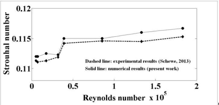
In Fig. 1 the Strouhal number values obtained numerically are reported together with those obtained in the wind tunnel test performed by Schewe (2013). For every simulation performed, the Strouhal number is calculated as St = (fs D) / U∞, where the shedding
frequency fs is computed by the time history of the fluid velocity at the two different points
placed in the wake of the body. From Fig. 1 it can be seen that the Strouhal number values calculated from the numerical simulations range between values of 0.11 and 0.12, in good agreement with the experimental data.
3.3. Dynamic simulations
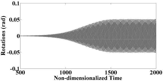
The aerodynamic fields and the structural motion of the body in dynamic conditions (as previously defined) are simulated simultaneously and in a coupled manner for two different undisturbed wind velocity values. In Fig. 2 the time history of the torsional displacements
obtained for a wind reduced velocity U = 4.58 (U = U / (fB), where f is the torsional
vibration frequency of the body) is shown. In agreement with the results shown by Liu et al. (2012), for this wind reduced velocity the body exhibits the flutter behaviour. In particular,
46 coherently with that obtained numerically by the above authors, there is a phase in which the amplitude of the torsional displacements gradually increases, followed by a phase in which the amplitude of the same displacements reaches a nearly constant value. The simultaneous and coupled simulation of the aerodynamic fields and the structural motion is also performed
for a wind reduced velocity U = 3.05. According to the experimental findings of the latter
authors, from the numerical simulation it emerges that the amplitude of the oscillations of the body is substantially stable for this wind reduced velocity. In particular, in Fig. 3 the time history of the torsional displacements obtained from the simulation performed for this wind reduced velocity is shown: from Fig. 3, it can be seen that in this case the torsional displacements are very small.
47 Figure 1. Strouhal number of the slender body with rectangular cross-section vs Reynolds number
Table 1. Geometrical and structural parameters of the slender body with rectangular cross-section
Width 0.04 m
Maximum depth 0.008 m
Torsional damping ratio 0.50%
Heaving damping ratio 0.50%
Natural torsional frequency 180 Hz
48 Figure 2. Time history of the torsional displacements of the slender body with rectangular cross-section
(U = 4.58)
Figure 3. Time history of the torsional displacements of the slender body with rectangular cross-section
49
Chapter 4
Test case 2: Forth Road Bridge deck
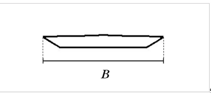
In this chapter, the aerodynamic fields which develop around the Forth Road Bridge deck in its current configuration (Configuration I). In Fig. 4 the geometric characteristics of the Forth Road Bridge deck in the current configuration are shown. The dynamic validation of the model (i.e. under the assumption that the cross-section is free to oscillate in the bending degree of freedom and in the torsional degree of freedom) is performed by comparing numerical and experimental results.
The simulations used for the dynamic validation are performed for increasing Reynolds number values (7.3 ˣ 103 < Re < 1.2 ˣ 104). In Table 3 the values of the geometrical parameters (overall width and maximum depth) and the structural parameters (mass per unit length and mass moment of inertia per unit length, natural heaving frequency and natural torsional frequency, heaving and torsional damping ratios) of the Forth Road Bridge deck are listed. In order to perform the integration of the fluid motion equations near the wall without excessive computational costs, the simulations have been performed at a reduced scale (1:780).
50 4.1. Geometry and numerical modelling
The results related to the bridge deck in its current configuration are obtained by using a block-structured grid which is made up of 33850 cells. In this grid, a geometric progression of 1.02 for the cell size varying is used in all directions. The dimensions of the computational domain in the x and y directions are respectively equal to Dx = 8B e Dy = 4B (being B the width of the cross-section of the reduced-scale deck). For every simulation performed, the undisturbed wind velocity U set at the domain inlet derives from the Reynolds number used,
the actual kinematic viscosity ( = 1.23 ˣ 10-5 m2/s) and the width B of the reduced model
cross-section. For the simulation performed at Re = 1.0 ˣ 104, at the solid walls the average value of the non-dimensional height y+ is close to 4 and the maximum value is close to 11.
4.2. Initial conditions for the stability analysis
The initial conditions in the stability analyses must be treated carefully. The instantaneous application of the full wind speed to an initially stationary structure leads to large transient initial motions from which it is difficult to extract definitive conclusions about the stability of small oscillations. To eliminate this problem, (according to Frandsen, 2004) for every simulation the structural damping values are set close to the critical values for the first instants of the simulation until the structure settles into a near-stationary configuration,
51 after which the damping values are changed to their estimated values. During this transient phase, the stiffness constants of the vertical and torsional spring are gradually relaxed from magnified values to those calibrated to give the correct natural frequencies in the fundamental modes.
In Fig. 5 the time histories of the torsional displacements and the vertical displacements
produced for a reduced wind velocity U = 6.0 are shown. From the figure it can be seen that,
during the first instants of the simulation (t < 0.08) in which the structure is gradually released, the gravity centre slightly drifts downward from the equilibrium position and the deck slightly rotates in a clockwise direction. In the instants immediately after t = 0.08 the structure continues to rotate clockwise, so much so that the wind angle of attack exceeds the value for which the resultant of the aerodynamic forces and, consequently, the vertical displacement of the gravity centre change direction (from downward to upward). From the figure itself it can be seen that the oscillatory motion produced after this transient phase shows a slow but constant decay of both the vertical and angular displacements: the value of
the imposed wind velocity (U = 6.0) lies under the critical flutter wind velocity value. In Fig.
6 the time histories of the rotations and the vertical displacements obtained for a reduced wind
velocity U = 7.0 are shown. In both cases, a constant growth of the displacements is
observed: the value of the imposed wind velocity (U = 7.0) lies above the critical flutter wind
52 the instantaneous values of the rotation oscillate is not fixed, but increases (in absolute value) going from the first to the second case. It follows that also the mean wind angle of attack
increases (in absolute value) going from the first to the second case. Specifically, for U = 6.0
the instantaneous values of the wind angle of attack oscillate around a mean angle of attack
roughly equal to -0.019 rad, whilst for U = 7.0 the instantaneous values of the wind angle of
attack oscillate around -0.027 rad. Consequently the aerostatic vertical displacement, which is due to the aerostatic component of the wind load, increases from about 0.013 to about 0.05, i.e. more than linearly with the square of the wind velocity.
4.3 Dynamic validation
The model validation is performed by comparing the numerical results with those obtained from the wind tunnel tests described in Robertson et al. (2003). Fig. 7 shows the plot
of the growth/decay rate of the rotations against the reduced velocity U of the wind (U = U /
(f B), being f the natural torsional frequency of the deck). From Fig. 7 it can observed that
the reduced critical velocity obtained by the presented model is U* = 6.12 (which
corresponds to a full-scale critical wind velocity of 76.5 m/s). This value matches well the
experimental result of U* ≈ 6.35 reported in Robertson et al. (2003). Furthermore, the
53 considered reduced velocities U. In agreement with that reported in Robertson et al. (2003),
it is found that at the point of flutter instability the frequencies of the translational and rotational motion are identical.
54 Figure 4. Forth Road Bridge deck cross-section in its construction state configuration
(Configuration I)
Table 3. Geometrical and structural parameters of the Forth Road Bridge deck (Robertson et al., 2003)
Overall width 31.2 m
Maximum depth 3.2 m
Mass moment of inertia per unit length 2.13 x 10⁶ kgm2/m
Mass per unit length 17.3 x 10³ kg/m
Torsional damping ratio 0.14%
Heaving damping ratio 0.31%
Natural torsional frequency 0.4 Hz
Natural heaving frequency 0.174 Hz
55 Figure 5. Time history of the vertical displacements (a) and the torsional displacements (b) of the Forth
56 Figure 6. Time history of the vertical displacements (a) and the torsional displacements (b) of the Forth
57 Figure 7. Growth/decay rate of the rotations of Forth Road Bridge deck vs reduced velocity
58
Chapter 5
Aeroelastic stability study of the Forth Road Bridge deck
In this section, the presented simulation model is utilised to analyse the full fluid-structure interaction of the Forth Road Bridge deck in the current configuration. A deep insight into the analysis and the detailed representation of the different phenomena that produce the onset of flutter for long span bridge decks with streamlined cross-section is proposed. In particular, at first it is identified the type of coupled flutter to which the Forth Road bridge deck is prone. It is then demonstrated that the reason for the onset of the torsional-branch coupled flutter lies in the fact that, within each of the first oscillation cycles, there is a portion of the cycle in which the energy supplied by the aerodynamic field to the deck motion is more than the energy extracted in the rest of the cycle. Lastly, it is shown that the reason for the amplification of the instability resides in the drifting of large vortical formations along the deck surface.
5.1 Coupled flutter type characterisation
In order to characterise the type of coupled flutter to which the Forth Road Bridge deck
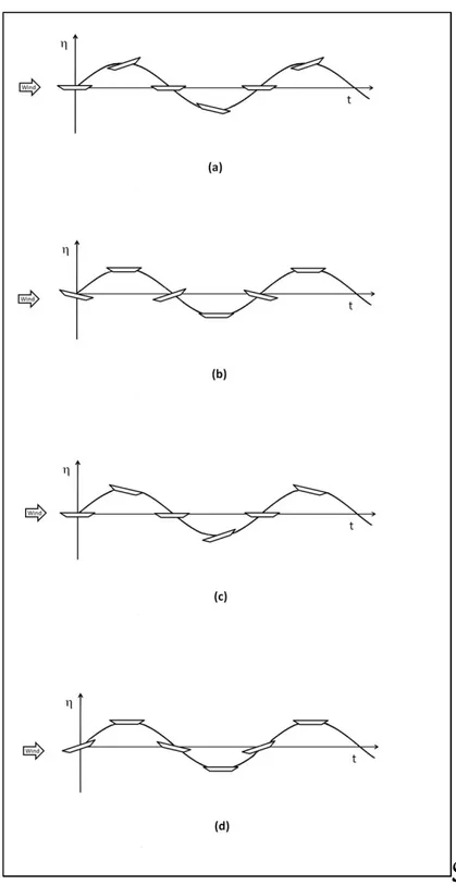
59 phase lag of the heaving response (vertical displacements) to the torsional response (rotations) of the structure is used. The latter authors highlight that the motion of a deck cross-section undergoing coupled flutter can be regarded as the superimposition of two fundamental oscillatory motions: the torsional fundamental mode and the heaving fundamental mode. The first one (torsional fundamental mode) is defined as a substantially torsional oscillatory motion around a certain point apart from the mid-chord point, accompanied by a vertical
oscillatory motion of small entity. In the torsional fundamental mode, the phase angle is
equal to 0° or 180° depending on whether the centre of rotation is placed upstream or downstream the mid-chord point of the deck cross-section (see Figs. 8(a), 8(c)). The second fundamental oscillatory motion (heaving fundamental mode) is defined as a substantially vertical oscillatory motion accompanied by a torsional oscillatory motion of small entity. In
the heaving fundamental mode, the phase angle is equal to 90° or -90° depending on
whether the sign of the small rotation of the upward moving cross-section is clockwise or anti-clockwise (see Figs. 8(b), 8(d)). That said, the relative contributions of the torsional fundamental mode and the heaving fundamental mode to the structural instability are
respectively quantified as the absolute values of the cosine and the sine of the above angle .
According to the treatise of the above authors, the torsional branch (TB) coupled flutter is defined as a coupled (torsional-flexural) flutter instability dominated by the fundamental torsional mode previously defined. In the case under examination (Forth Road Bridge in its