Università degli Studi di Ferrara
DOTTORATO DI RICERCA IN
"ECONOMIA"
CICLO XXVIICOORDINATORE Prof. Massimiliano Mazzanti
IMPACTS OF CO
2
TAX
ON
ITALIAN ECONOMY
A COMPUTABLE GENERAL EQUILIBRIUM APPROACH (CGE)
Settore Scientifico Disciplinare: SECS-P/01
Dottorando Tutore
Deldoost Hosseini Seyed Mostafa Mazzanti Massimiliano
2
“When I began the study of economics some forty one years ago, I was struck by the
incongruity between the models that I was taught and the world that I had seen growing up”
Nobel Prize Winning Economist Joseph Stiglitz
ABSTRACT
Anthropogenic CO2 emission is one of the chief greenhouse gases that coming from the burning of fossil fuels by households and firms imposing a cost and negative impact on present and future generations in the form of climate change and global warming. There are many ways and instruments to reduce fossil fuel emissions. Making pollution expensive by imposing tax would be one way to motivate consumers and producers to continuously substitute fuels with high carbon content by alternative with low carbon content.
This paper uses a top-down static Computable General Equilibrium (CGE) model for a small open economy to analyze the effects of carbon tax policy on Italian macroeconomic variables. Standard assumptions of CGE models are employed. By considering various direct and indirect effects, CGE models are appropriate for analysis policies like CO2 reduction, which generate significant direct and indirect impacts. Our approach at this study is to apply CO2 tax instrument as a result of burning input fossil fuel into production function.
The empirical basis for the model is a Social Accounting Matrix (SAM) that consists of several production sectors which employ primary factors as well as intermediate inputs to produce goods (output) for the domestic and foreign market. Domestic demand includes intermediate demand and final demand. The domestic goods are used as intermediate inputs in production processes or consumed by final users like households, government, and investment sector.
There are 57 production sectors in GTAP1 database version 7, 2004 which are aggregated into five production sectors, one household, government, and the rest of the world. WIOD 2environmental accounts are used which consist of information on energy consumption that has broken down into a number of energy carriers. The model is formulated using GAMS3 and solved with the PATH4 algorithm.
Results show that reducing CO2 emissions through carbon tax instrument would have small negative effect on GDP and consumer welfare i.e. consumer’s real income. Under a carbon-tax-compensation by redistribution back to the household, welfare loss is lower and economy is less adversely affected by higher prices. We use different values on key exogenous elasticity
1Global Trade Analysis Project 2 World Input output Database 3 General Algebraic Model System
3
parameters to ensure the robustness and the reliability of the model. Sensitivity analysis results illustrate that our model is robust and reliable with respect to most parameters’ value.
The Kyoto protocol has fixed the base year (1990) CO2 emissions for Italy to 436 million s. In order to meet Kyoto target, Italian sectors should reduce CO2 emission around 1.2 millions in each following year. Our simulation results show that by imposing tax between 5 and 10 dollar per tCO2 (18.35 and 36.7 dollar per carbon) Italy could meet the Kyoto target by 2012 and this rate should rise through time gradually to meet second commitment (CP2) target as well. However, as reported by European Environment Agency (2014), Italy’ GHG is not fully on track towards its burden-sharing target and need to purchase additional international credits before the end of the true-up period.
Key words: Carbon tax, Italy, Computable General Equilibrium (CGE), Social accounting matrix (SAM), Input output multipliers, GAMS
4
ACKNOWLEDGMENTS
This dissertation would not have been possible without the support and help of many people. First and foremost, I wish to express appreciation and gratitude to Professor Massimiliano Mazzanti for his guidance during my doctoral program at the Ferrara University. I am also extremely indebted to IUSS, for the support provided to me for my research.
Thanks to Professor James Markusen, I visited him at ETH University, Zurich. I really enjoyed from his workshop and learned a lot about GAMS programming. I would also extremely thankful to Professor John Wagner and Professor Pablo Martinez for their help. To my friend Dr. Haqiqi, I am thankful for knowing and learning from you.
Confucius said: "During your parents' lifetime, do not journey afar. If a journey has to be made”, you must have convincing reasons. I owe to my parents who have given me encouragement for PhD journey.
A special thanks of course to my beloved family: my wife Forough and my son Yashar for the continuing love, faith and infinite support.
I am also grateful to my oncologist Dr. Alessandra Santini for her care and kindness as well as God for giving me sufficient strength to overcome my problems and complete this thesis.
Publications
Calculation of Emission Multipliers in Italy, Spain and Germany (1995–2009). An Environmental Input Output Analysis. Warsaw School of Economics Press ISBN 978-83-7378-940-1
A 2004 Social Accounting Matrix (SAM) analysis for Italy Impacts of carbon tax on Italian economy: A CGE approach
5 TABLE OF CONTENTS
Chapter 1
1.1 INTRODUCTION ... 11
1.2 Objectives and research questions... 14
1.3 Methodology... 14
1.4 Outline of the Thesis ... 14
Chapter 2 2.1 Energy and Environment facts in Italy and Europe... 16
2.2 Energy and Environment facts in Italy and Europe... 20
2.3 ETR and Double Dividend Approach ... 22
2.4 Tradable permits ... 25
2.5 Carbon Tax ... 26
2.5.1 Carbon emissions calculation... 29
2.6 Review of previous studies ... 34
Chapter 3 3.1 Foundation of the CGE model ... 37
3.1.1 Introduction ... 37
3.1.2 Framework of CGE models ... 38
3.1.3 Advantages and disadvantages of CGE models... 40
3.1.4 Application of CGE models ... 41
3.1.5 Key steps for constructing CGE model ... 41
3.1.6 CGE model Classification... 43
3.1.7 Top down vs. Bottom-up models ... 44
3.2 Some of microeconomics theory in CGE modeling ... 45
3.2.1 Envelope theorem ... 46
3.2.2 Profit function and Hotelling lemma ... 48
3.2.3 Expenditure minimization and Shephard lemma ... 48
3.3 Algebra of a AGE model : N Sectors, N commodities ... 49
6
3.4.1 General Form of Mathematical Relations in Computable General Equilibrium
Models…. ... 51
3.4.2 Calibration of CGE Models ... 60
3.5 Model Assumptions ... 64
6.3 Mathematical Relations of Static CGE Model ... 65
3.6.1 Nested Structure of Production Cost in Different Activities ... 66
6.3.3 Intermediate Goods’ Demand ... 70
3.6.3 Import Optimmization Behavior ... 71
3.6.4 Export Optimization Behavior ... 72
6.3.3 Good’s Market Equilibrium Condition ... 73
6.3.3 Equilibrium (Clearing) Condition in Markets for Factors of Production ... 74
3.7 Casting the General equilibrium model into GAMS ... 74
Chapter 4 4.1 The CGE model database: Social Accounting Matrices (SAM) ... 76
4.1.1 Basic SAM accounts ... 78
4.1.2 SAM development ... 80
4.2 I/O and SAM multiplier... 83
4.3 Data... 84
4.4 Microeconomic and Macroeconomic data in a SAM ... 87
4.4.1 Italy’s Gross Domestic Products for 2004 ... 87
4.5 The analysis of I/O and SAM multipliers ... 91
4.6 Backward and Forward linkage analysis ... 92
4.6.1 Classifying Backward and Forward Linkage Results ... 95
4.7 Summary of SAM and Italy’s SAM analysis ... 96
Chapter 5 5.1 Model Simulation and Results analysis ... 98
5.1.1 Independent carbon tax scenario... 99
5.2 Sensitivity analysis ... 101
5.2.1 Carbon tax revenue recycling scenario ... 105
7
5.4 CONCLUSION AND RECOMMENDATION ... 108
REFERENCES ... 111
Appendix 1 : Activity abbreviation ... 119
Appendix 2: The concordance between WIOD, GTAP, OECD and ISIC rev.3.1 code ... 120
8
ILLUSTRATION
LIST OF FIGURES
Figure 1-1 Global mean temperature ...11
Figure 1-2 The Growth of global CO2 emissions ...12
Figure 1-3 Emissions from the major emitting countries ...13
Figure 1-4 Thesis Outline ...15
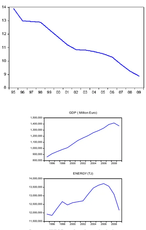
Figure 2-1 Energy Intensity (TJ / Million Euro) ...17
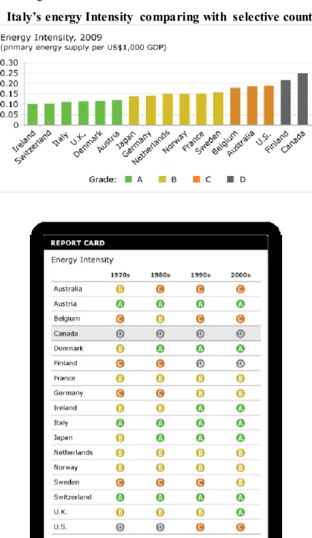
Figure 2-2 Italy’s energy Intensity comparing with selective countires ,2009 ...18
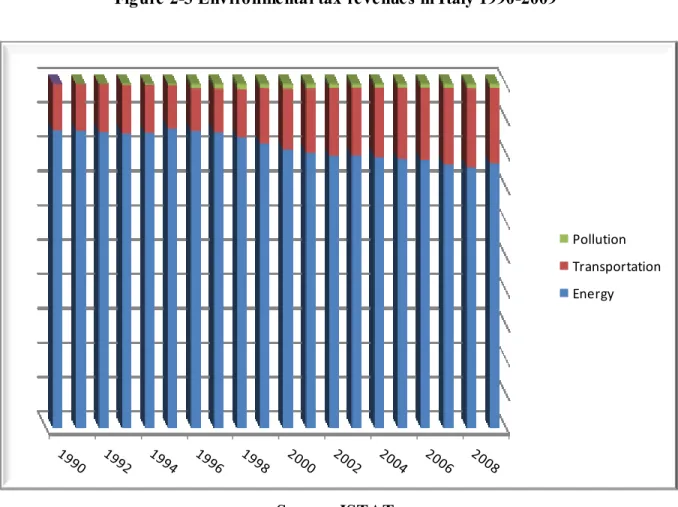
Figure 2-3 Environmental tax revenues in Italy 1990-2009 ...21
Figure 2-4 Total Environmental tax Revenue in Italy and EU15 ...22
Figure 2-5 CO2 (1000 Tone) ...28
Figure 2-6 Energy intensity and CO2 intensity 1995-2009 ...28
Figure 3-1 Circular flow in a CGE model ...39
Figure 3-2 Key issues in CGE model (Steps towards a policy experiment with CGE models) .42 Figure 3-3 Computable General Equilibrium Classification ...43
Figure 3-4 Top Down, Bottom up and Hybrid model ...45
Figure 3-5 Visual explanation of the Envelope theorem for Parabola function ...47
Figure 3-6 : Nested Production Function...67
Figure 3-7 : Nested households consumption structure...69
Figure 4-1 Direct and indirect sector linkage ...93
9 LIST OF TABLES
Table 2-1 Main energy trend in ITALY ...16
Table 2-2 Italy’s priority policy objectives ...19
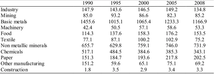
Table 2-3 Energy intensity in industry and in BEN sub-sectors ...19
Table 2-4 Environmental taxes by European Commission classification ...20
Table 2-5 Labor Tax versus Environmental Tax in member State...24
Table 2-6 Carbon dioxide taxation in different countires...27
Table 2-7 Carbon Emission Factors in Different Units ...30
Table 2-8 Energy Equivalent Conversions ...30
Table 2-9 List of energy commodities included in the WIOD database ...31
Table 2-10 Gross energy use by sector and energy commodity (Terajoules) ...32
Table 2-11 Emission relevant energy use by sector and energy commodity ...32
Table 4-1 Standard macro SAM structure used in CGE model...77
Table 4-2 Traditional SAM layout ...78
Table 4-3 Endogenous accounts of aggregated industry ...81
Table 4-4 Concordnace between GTAP, WIOD and author aggregation code ...85
Table 4-5 Italy’s SAM 2004 ...86
Table 4-6 Structure table –Factor cost shares ...88
Table 4-7 Structure table-Industry shares in factor employment ...88
Table 4-8 Structure tabel- Commodity shares in domestic demand and trade ...89
Table 4-9 Tax structural table ...90
Table 4-10 Type I multipliers in open model ...91
Table 4-11 Type II multipliers in closed model ...91
Table 4-12 SAM multipliers ...92
Table 4-13 Classification of backward and forward linkage ...96
Table 4-14 Linkage results, Italy 2004 data ...96
Table 5-1 Percentage changes of macroeconomic variables , energy usage and CO2 emissions under different tax rate Cobb Douglas production function (S:1) ...100
Table 5-2 Percentage changes of supply (production) under different tax rate Cobb-Douglas production function (S:1)...101
Table 5-3 Percentage changes of macroeconomic variables , energy usage and CO2 emissions under different tax rate Lower elasticity of substitution (S: 0.5 )...103
10
Table 5-4 Percentage changes of macroeconomic variables , energy usage and CO2 emissions under different tax rate Higher elasticity of substitution (S: 1.5) ...104 Table 5-5 Percentage changes of supply (production) under different tax rate Lower elasticity
of substitution (S: 0.5) ...104 Table 5-6 Percentage changes of supply (production) under different tax rate higher
elasticity of substitution (S: 1.5) ...104 Table 5-7 Percentage changes of macroeconomic variables , energy usage and CO2 emissions
under different tax rate Cobb-Douglass production function (S:1) ...105 Table 5-8 Percentage changes of supply (production) under different tax rate Cobb-Douglas
production function (S:1)...106 Table 5-9 GHG and CO2 Italy’s emission (Million tone) ...107
11
Chapter 1
1.1 INTRODUCTION
"We have forgotten how to be good guests, how to walk lightly on the earth as its other creatures do."
Barbara Ward, Only One Earth, 1972.
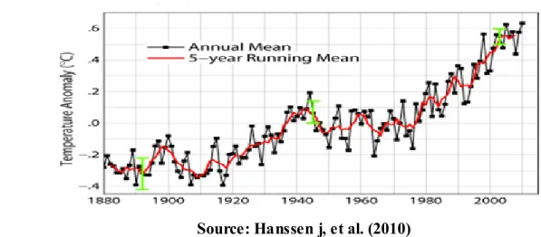
In this century, our home planet is in crisis, because for many years, humankind had an imperfect responsiveness of its relationship with the natural environment. Nowadays, we are vigilant those natural resources are limited and that our actions affect the ecosystem. Currently, our earth and its guest are faced with a problem of global warming and climate change. Figure 1-1 shows the history of global mean temperature versus time. Scientist anticipate by the year 2100 our planet’s temperature will be increased by 3 to 4 Celsius degrees, if current energy consumption continue, consequently we face with melting ice caps and sea level rise between 30 and 110 cm, even a rapid stabilization CO2 at 450 ppm1 will generate temperature change approximately 2○ C (IPCC Synthesis report); thus people who lives in coastal and equatorial areas as well as vulnerable places such as Netherlands, Bangladesh and Egypt are at risk with flood, storm surge. This event can drown out several islands as well.
Figure 1-1 Global mean temperature
Source: Hanssen j, et al. (2010)
12
Energy especially fossil fuels plays an important role in overall GDP growth and still a crucial input for producing goods and services both in developing and developed countries. As a result economic growth and energy consumption persist to be closely interrelated.
When fossil fuels such as coal, gas and oil are burned they react with oxygen and produce carbon dioxide (CO2). Carbon dioxide is one of the numerous heat-trapping greenhouse gases (about 77% of the volume of GHGs) emitted into atmosphere (with a longer lifetime in
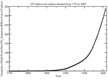
atmosphere ) through anthropogenic activities in indifferent ways, mostly by the combustion of fossil fuels and deforestation. Carbon dioxide (CO2) is added in various steps during the production of goods especially in pollutant industrial sectors like: pulp, cement, glass, and so on. Most of this gas is produced by the combustion of fossil fuels in energy intensive sectors and creates climate changes and global warming. These gases are main cause of current global challenge commonly referred to climate change furthermore negatively affect human life. Historical trends in Carbon dioxide (CO2) emissions figure1-2 show that worldwide emissions of CO2 have raised steeply since the start of the industrial revolution. According to CDIAC 1(2010) approximately 337 billion metric tons have been released to the atmosphere since 1751 and about 50% of this gas has emitted since mid-1970s.
Figure 1-2 The Growth of global CO2 emissions
Source: CDIAC (2010)
1 Carbon Dio xide Information Center
13
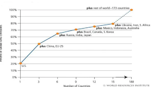
Figure 1-3 shows the emissions from major emitting countries contribute to the world total. It goes without saying that, just a few countries are responsible for 80% of the world’s greenhouse gas emissions accordingly developed countries tend to produce more emissions than developing countries. However, it is anticipated that between 2020 and 2030, carbon dioxide emissions from energy consumption at developing countries will exceed those of developed countries due to dealing with poverty and other social challenge a t their economic growth process. Developing countries can justify this issue and can say to developed countries that “you created problem, you fix it”1. This position from them is completely understandable but finally who will take responsibility for climate change issue? So it is better to be rational and forget about who caused the problem, this phenomenon is a global problem and all countries- whether developed or developing- require global cooperative actions.
Figure 1-3 Emissions from the major e mitting countries
Different policy instruments have been established to protect natural environment, human life as well as reduce the dependency on energy, most notably on fossil fuels.
One possible instrument to reduction of greenhouse gas emissions especially carbon dioxide is the taxation of CO2 emissions. It is clear that pricing carbon will significantly impact on industries and end users in form of higher marginal cost and commodity price re spectively.
1 US constitute less than 5 % of global population but use about 24 % of world’s energy. US resident use energy much greater than Chinese and Indian. They emit 6 times more GHG than the Chinese and 18 times more than the typical Indian.
14
Carbon tax would lead to decrease of the demand thereof, lastly leading to a reduction of the CO2 emission level.
1.2 Objectives and research questions
The purpose of this research is to explore the effects of imposing carbon tax policy on Italian economy by simulating different scenarios. We will focus on CO2 emissions from the fossil fuel energy users, so the main questions addressed in this research are:
Q1: What are the impacts of carbon tax on Italian macroeconomic variables? We consider the impacts on variables such as: industry-by-industry output level, households and governmental consumption, social welfare, and foreign trade.
Q2: What range of carbon tax is required to achieve Italian Kyoto target?
We will provide a quantitative answer to each of these broad set of questions in the Italian context. Some more particular objectives are:
Provide a literature review of previous research on the carbon tax
Collect and compile Italy SAM from GTAP database and convert into standard form for construction of CGE models
Prepare computer programs for numerical simulations in GAMS
Conducting policy simulations with the models and interpret the simulation results
1.3 Methodology
A static top down computable general equilibrium (CGE) model of the Italy economy is constructed for this research. Carbon tax is implemented on the intermediate demand for fossil fuels .The model consists of five industries, one representative household, government, two factor inputs, and a trade system.
1.4 Outline of the Thesis
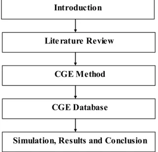
A brief outline of the procedure used to write this research is shown in figure 1-4. This dissertation is organized into four more chapters following this introduction. First we shall start by giving a review of energy and environment facts in Italy then go to review environmental tax reform (ETR) in Europe as well as introduce two common reductions of
15
CO2 emissions instruments from fossil fuels: tradable permits and carbon tax. In chapter three the general structure of computable general equilibrium (CGE) as well as some microeconomic theory which play dominant role in CGE modeling are discussed then the chapter goes on to focus on algebra and functional forms of CGE model that representing behavior of different individual agents and mathematical statement of model. Chapter 4 will review conceptual framework and general structure of social accounting matrix that we used in building model. In the following we calculate key macroeconomic indicators in SAM database as well as explain how input output and SAM multipliers are calculated and analyzed. We describe how Rasmussen backward and forward linkages are calculated in order to identify the most important sector in Italy’s economy
Finally, Chapter 5 will expose the different simulation policy scenario to assess the impact of carbon tax on Italy’s macroeconomic variables and will provide a clear answer to the research questions.
Figure 1-4 Thesis Outline Lite rature Review
CGE Method
CGE Database
Simulation, Results and Conclusion Introduction
16
Chapter 2
“The art of taxation consists in so plucking the goose as to obtain the largest amount
of feathers with the least possible amount of hissing”
Jean -Baptiste Colbert
2.1 Energy and Environment facts in Italy and Europe
Italy is the tenth largest economy in the world in terms of GDP measured at purchasing power parity (PPP) as well as largest energy consumers among European countries (IEA, 2010). According to Energy Charter (2009) the traditional fossil fuels – oil, natural gas and coal -account for 87.5% total primary energy supply (TP ES). More than 85% of this energy source is imported.
Oil and gas are still the dominant resource of providing 78.5 % of total energy. The amount and Percent share of TPSE in 2007 were: Oil 82 MTOE (42.5%), gas 70 MTOE (36%), Coal 17.5 MTOE (9%), electricity and renewable energy (12.5%).
Table2.1 shows the main energy trends in Italy from 2002 to 2007.
Table 2-1 Main energy trend in ITALY
Parameter 2007 2002/2007
Growth Rate
GDP (Euro million 2000) 1.284.868 +5.5%
TPES (MTOE) 194.45 +3.4%
Primary Energy Intensity
(TOE/Euro million 2000) 151.4 -1.9%
Electricity Intensity
(TOE/Euro million 2000) 20.70 +3.5%
SOURCE: ISTAT
Also below graphs shows GDP and Energy trends in Italy from 1995 to 2009.
Energy intensity is proxy for efficiency of a nation’s economy. It is calculated as units of energy per unit of GDP, in other words quantity of energy required to produce one unit of output (GDP); thus less energy intensity means consuming less energy to obtain the same products and services.
Mathematically:
17
This indicator can be computed both physically and financially. When output is measured in Physical units like liter or s, energy consumption or energy input is expressed in energetic units, for example MJ / tone. On the other hand, when output is measured in monetary units, this indicator is calculated by energy consumed divided by dollar value of output like: TJ / GDP in €. Figure 2-1 shows the trend of the energy intensity in Italy from 1995 to 2009.
Figure 2-1 Energy Intensity (TJ / Million Euro)
Source: WIOD and author calculations
800,000 900,000 1,000,000 1,100,000 1,200,000 1,300,000 1,400,000 1,500,000 1996 1998 2000 2002 2004 2006 2008 GDP ( Million Euro) 11,500,000 12,000,000 12,500,000 13,000,000 13,500,000 14,000,000 1996 1998 2000 2002 2004 2006 2008 ENERGY (TJ)
18
Another kind of indicator is energy efficiency which is often used interchangeably with energy intensity, but the different between them is significant. Simply energy efficiency is the inverse of the energy intensity. It should be noted that, for analyzing trends in energy efficiency over time a common indicator that used widely is energy intensity. For example declining of energy intensity in specific period reports improvement in energy efficiency.
As we can see from the below graph, in 2009, Italy ranks in the third place out of 17 peer countries and earns “A” grade.
19
Moreover, figure 2-2 Illustrates that Italy was leading in the Europe and got top qua rtile of energy intensity in the period 1970s to 2000s; now this index is 15% lower than EU average Reducing energy intensity was principally strategic goals with highest priority of Italian policy maker in order to reducing dependence of energy imports. The following table indicates the priority of Italy’s policy objectives.
Table 2-2 Italy’s priority policy objectives
Policy Objective Priority
Reduce total final consumption / GDP 1
Reduce dependency on energy imports 2
Diversification of fuels 3
Reduction of 5
Increase utilization of indigenous primary energy sources 4 Source: Regular Review of Energy Efficiency Policies
At the industrial level energy intensity is defined as energy consumption in physical units (Ei) by Sector (i) divided by value added (Yi). In mathematics form:
2.2 ) In spite of reduction in final energy consumption in Italian industrial sector from 33.6% in 1990 to 28.7 % in 2008 but more than one quarter of total energy still has been consumed by industry sector (Buzzigoli and Viviani, 2012). Table2-3 shows the energy intensity (koe/ 1000 Euro) in Italian industries and National Energy Balance (BEN) classification.
Table 2-3 Energy intensity in industry and in BEN sub-sectors
1990 1995 2000 2005 2008 Industry 147.9 143.6 146.5 149.2 134.8 Mining 85.0 93.2 86.6 82.3 85.2 Basic metals 1455.6 1015.1 1065.4 1233.3 1166.9 Machinery 42.4 50.5 57.1 58.6 53.3 Food 114.3 137.6 158.3 176.2 153.5 Textile 77.1 87.1 100.2 102.9 75.2
Non metallic minerals 655.7 629.8 759.1 746.0 731.9
Chemicals 517.1 484.5 384.6 385.3 343.1
Paper 151.3 184.7 193.6 217.8 202.5
Other manufacturing 151.2 59.6 65.1 75.1 69.2
Construction 1.8 3.5 2.9 3.4 3.3
20
2.2 Energy and Environment facts in Italy and Europe
Climate change, ecosystem degradation, deforestation, the impact of variety pollution on human health is the most current concern in environmental sustainability subject. Because of this as well as other reasons, there is a worldwide consensus to finding solutions to alleviate global warming.
Green (environmental) taxation policy instrument has been widely discussed in the last two decades. The objective of this tax is used to enhance environmental protection and control any kinds of pollution as well as collecting revenues simultaneously. Environmental taxation can defined as “compulsory payments levied on tax bases deemed to be of particular environmental relevance “(OECD, 2001). It can be categorized into i) energy taxes ii) taxes on pollution and resources and iii) energy taxes.Table2-4 presents detailed classification of those taxes in Italy according to the European Commission’s categories.
Table 2-4 Environmental taxes by European Commission classification
Energy
Excise duty on mineral oils In-bond surcharge on mineral oils
In-bond surcharge on liquefied petroleum gases Excise duty on liquefied petroleum gases Excise duty on methane
Local surcharge on electricity duty Excise duty on electricity
Tax on coal consumption
Transport
Motor vehicle duty paid by households Motor vehicle duty paid by enterprises Public motor vehicle register tax (PRA) Provincial tax on motor vehicles’ insurance
Pollution
SO2 and NOx pollution tax
Contribution on sales of phytosanitary products and pesticides Regional special tax on landfill dumping
Provincial tax for environmental protection Regional tax on aircraft noise
21
Figure 2-3 shows environmental tax revenues in Italy in 1990 until 2008 in three main categories. Throughout (over) this period, the revenue from taxes related to energy was about 82% of total environmental taxes. Energy tax revenues have raised from 19.3 billion to 31.7 billion euro in 2009, or about 2.6 GDP percent. Oil demand is increasingly concentrated in the transportation sector in Italy (IEA, 2010), for this reason government decided to increase tax rate in transportation sector thus revenue from transportation fuel taxes increased approximately from 3000 million to 9000 million euro between 1990 and 2009 (ISTAT,2010). Resource and pollution taxes represented small shares about 1% of the total in Italy.
Figure 2-3 Environmental tax revenues in Italy 1990-2009
Source: ISTAT
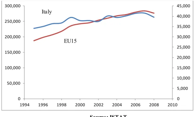
Figure2-4 shows that the total revenue from environmental taxes in EU15 and Italy between 1995to 2008. As can be seen in the below figure environmental tax revenue in EU and Italy increased this period except 2008 due to economic crisis.
Pollution Transportation Energy
22
Figure 2-4 Total Environme ntal tax Revenue in Italy and EU15
Source: ISTAT
The reduction of greenhouse gas emissions (GHG) has been undertaken in European countries during the 1990s, in recognition of serious environmental challenges. Some countries like Finland, Sweden, and Denmark pledged soon to curb CO2 emissions by up to 20 % by introducing unilateral carbon tax.
In Italy, Japan and New Zealand, carbon energy taxation emerged in political agenda in governmental section by applying environmental tax reform (ETR) which is vital to assist sustainable macroeconomic, environment protection also crucial to low carbon growth in European Union. In broad sense,” ETR includes the establishment of environmental tax, the reformation of fiscal policies related with environment and natural resource, as well as the elimination of inappropriate subsidy and charge policies are adverse to environment”
(Cahzhong, et al.2012). ETR plays not only a significant role in environmental protection but also promoting economic agents behavior toward low carbon economy.
2.3 ETR and Double Dividend Approach
As part of greening of taxation systems, the Europe 2020 strategy emphasizes the potential of ETR, to shift tax burden from conventional taxes such as labor to environmentally damaging
0 5,000 10,000 15,000 20,000 25,000 30,000 35,000 40,000 45,000 0 50,000 100,000 150,000 200,000 250,000 300,000 1994 1996 1998 2000 2002 2004 2006 2008 2010 Italy EU15
23
activities such as resource use or pollution; simply as Delors1 recommendation ‘goods’ to ‘bad’. Clearly, one factor that has negative effect on employment is high taxes; by replacing some part of the tax with green tax in ETR approach it can lead to reduction in unemployment and boost employments in market.
In 1990s and 2000s some Scandinavian countries implemented ETR with broadly positive results. The consequence of ETR idea which is shift taxation –from labor to pollution-, lead to opportunities to improve not only employment but also tackle negative economic impacts. The study set up by Manersa and Sancho (2005) as well as Faehn et al. (2009) using a CGE model examines double dividend policy action in Spain. They concluded that, by imposing energy tax not only toxic gas emissions are reduced but also unemployment ra te would improve.
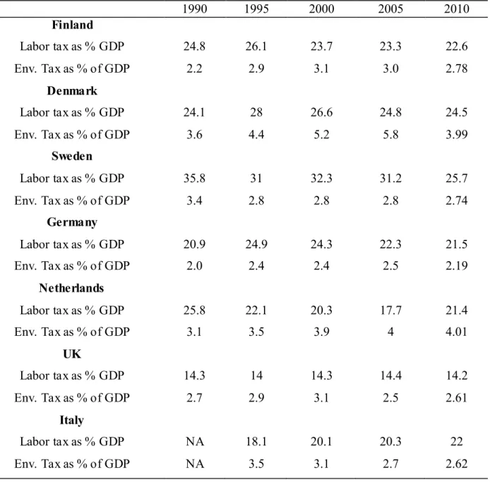
Generally speaking environmental tax revenue can provide two kinds of benefits that known as double dividend. First and most importantly is an improvement in environment and the second is improving economic efficiency through offsetting the extra cost of production. One way to evaluate achievement of the ETR objectives is comparing the trend labor taxation to GDP ratio with the environmental taxation to GDP (EEA, 2005).
Table 2-5 summarizes analysis of tax on labor versus environmental taxes in Finland, Denmark, Sweden, Germany, The Netherlands, UK and Italy between 1990 and 2010. Despite of fundamental motivations for implementing ETR in EU member states are similar; the approach of the respective tax shift program in terms of economic sector affected and recycling
Mechanism varies. The most common policy tool of ETR in EU members is carbon tax or energy consumption tax but UK for example introduced special tax like landfill taxation whereas Denmark and Dutch have increased existing tax on waste disposal.
In the late 1990s, Italy’s environmental tax was the highest level entire EU with a 3.5 percent out of GDP. But this edge subsequently scaled down and in 2010 environmental taxes
accounted 2.6 as a percent of GDP, just equaled the EU average.
In contrast, tax in Italian fiscal system increased from 18.1% to 22 % in the period 1995-2010 as a percentage of GDP. This tax accounted for 52% of total collected revenues in 2010
24
whereas consumption taxes in the same period were 10.2% and 10.6% with respect to GDP and below the European Union average.
Table 2-5 Labor Tax versus Environme ntal Tax in membe r State
1990 1995 2000 2005 2010 Finland Labor tax as % GDP 24.8 26.1 23.7 23.3 22.6 Env. Tax as % of GDP 2.2 2.9 3.1 3.0 2.78 Denmark Labor tax as % GDP 24.1 28 26.6 24.8 24.5 Env. Tax as % of GDP 3.6 4.4 5.2 5.8 3.99 Sweden Labor tax as % GDP 35.8 31 32.3 31.2 25.7 Env. Tax as % of GDP 3.4 2.8 2.8 2.8 2.74 Germany Labor tax as % GDP 20.9 24.9 24.3 22.3 21.5 Env. Tax as % of GDP 2.0 2.4 2.4 2.5 2.19 Netherlands Labor tax as % GDP 25.8 22.1 20.3 17.7 21.4 Env. Tax as % of GDP 3.1 3.5 3.9 4 4.01 UK Labor tax as % GDP 14.3 14 14.3 14.4 14.2 Env. Tax as % of GDP 2.7 2.9 3.1 2.5 2.61 Italy Labor tax as % GDP NA 18.1 20.1 20.3 22 Env. Tax as % of GDP NA 3.5 3.1 2.7 2.62 Source: ISTAT
But let us be realistic. Ecotax are complex mechanism because it should be balance not only between social and economic effect but also should consider political and public acceptance like income distribution or international competitiveness as well.
25
Manersa (2009) stated that, double divided in actual situation will not necessarily map with theoretical situation and it is highly influenced by model structure, behavioral rules of agents, government policies and many other parameters.
2.4 Tradable permits
Tradable pollution (or emission) permits are a cost-efficient, market-driven approach to controlling pollution caused by negative externalities. Tradable emission permits allow the central authority to decide how much tones of a toxic gas may be released into atmosphere over a specified interval of time by allocating licenses to individual firms to pollute at a certain level. The main type of allowance emissions trading is known as "cap and trade".
Governmental body sets an absolute pollution limit or cap on the amount of a pollutant that may be emitted.
By putting a price and giving financial value on emission permit companies as a seller and buyer can trade these permits on the stock market. If company “A” achieves a reductions goal which has been set by law or agreement, can benefit by sell permits to co mpany “B” that pollute higher than standard permit allow. The ability to sell permits incentives company “A” to invest in pollution abatement.
By far the first large multi-country and multi-sector emissions trading scheme for CO2 allowance in the world is The European Union Emissions Trading System (EU ETS) which launched in 2005 to combat climate change, and works on the ‘cap and trade’ principle. The system furnishes for interconnection with emission-reduction credit programs (ECR) in other countries such as the Kyoto Protocol’s Clean Development Mechanism (CDM) and joint implementation (JI).
The CDM and JI mechanism are two project- based defined in article 12 and 6 of Kyoto protocol respectively. The CDM mechanism allows private companies with emission reduction to fund an emission removal project in developing countries and earn tradable certified emission reduction (CER) units. Similarly, JI is a mechanism that allows for Annex I Parties to undertake and invest in emission reduction projects in any other Annex I Parties to generate Emission Reduction Units (ERU). Compared to tradable permits, the tax system is much easier to handle.
Although, cap and trade instrument gives government a macro control of pollutant volume but administrative, monitoring and enforcement cost may be high. This instrument is criticized by
26
ethicists for that the polluters are undue right to continue to burn fossil fuels, destroy forests and pollute communities (Lee, 2012).
2.5 Carbon Tax
Air pollution is most dangerous threats to our health and environment. Air pollution has been a problem throughout history. Even in ancient Rome Empire a Roman philosopher for instance, Seneca, complained about air pollution in Rome in 61 CE, he wrote:
“As soon as I had escaped the heavy air of Rome and the stench of its smoky chimneys, which when stirred poured forth whatever pestilent vapours and soot they held enclosed, I felt a change in my disposition.”
But since industrial revolution, the air quality became worse mainly as a result of burning fossil fuels. This matter will increase not only the occurrence of respiratory disease like asthma and other serious human health problem but also erode our environment. Carbon dioxide (CO2) is one of the chief greenhouse gases and responsible for driving climate change. In theory, the mitigation of CO2 emissions can be achieved through different instruments. A carbon tax is a form of explicit carbon pricing and a type of Pigovian tax levied on the carbon content of fuels. Carbon tax often expressed as a value per CO2 equivalent (per tCO2e). 1It is one of the most efficient instruments available to curb of carbon dioxide
emissions by providing a motivation for producers and consumers to substitute carbon- poor for carbon-rich flues that could be a feasible alternative. While such carbon taxes can raise significant amounts of revenue, it could also have negative effects and unintended
consequences on macroeconomic variables such as economic growth rate, income distribution, competitiveness of a country’s exports (Cuervo, J. and V. Gandhi, 1998), as well as adverse impacts on the distribution of welfare (Creedy,J and Sleeman,C,2005).
In order to stabilize energy consumption and decrease CO2 emissions, Finland and Netherlands in 1990, Norway and Sweden in 1991 were adopted carbon tax. Later other European countries such as Ireland (2010), Switzerland (2008) and Slovenia (1997) were implemented carbon tax which is levied on motor and heating oil. The average price of a carbon is relatively different from country to country .The highest tax rate in 2010 is related to Sweden by 103 € per of CO2 and lowest is related to eastern European countries like: Estonia
27
(2010), Latvia (2008) and Poland (2010) by 2, 0.2 and 0.1 euro per ton of CO2 respectively. The Table 2-6 provides an overview of CO2 tax in different countries.
Table 2-6 Carbon dioxide taxation in different countires
Country CO2 Tax
Australia $24.151 per tCO2e (2013)
British Columbia CAD30 per tCO2e (2012)
Denmark USD31 per tCO2e (2014)
Finland EUR35 per tCO2e (2013)
France EUR7 per tCO2e (2014)
Iceland USD10 per tCO2e (2014)
Ireland EUR 20 per tCO2e (2013)
Japan USD2 per tCO2e (2014)
Mexico Mex $ 10 -50 per tCO2e 2014 Depending on fuel type Norway USD 4-69 per tCO2e (2014) Depending on fuel type South Africa R120/tCO2 (Proposed tax rate for 2016)
Sweden USD168 per tCO2e (2014)
Switzerland USD 68 per tCO2e 2014
United Kingdom USD15.75 per tCO2e (2014)
Source: World Bank
In 2009, the total Italian CO2 emission was 424.765 kilo tone that industry sector and
households were responsible for 78% and 22 % respectively. Graph below shows the trend of CO2 in Italy from 1995 to 2009.
28
Figure 2-5 CO2 (1000 Tone)
Source: WIOD and author calculation
Over the first ten years since 1995, the CO2 emissions steadily increased and start to decrease from 2006. According to Kyoto protocol, EU member state should cut of 20% in GHG
emissions with respect to 1990 levels by 2020. Kyoto target for Italy is set at 485.1 metric tons of carbon dioxide equivalent for the first commitment period. According to official data
(APAT, 2007) in 2005, GHG emissions were 12.1% over 1990 levels. As reported by European Environment Agency (2014), “Italy is not still fully on track towards its burden-
sharing target under EU law thus Italy should purchase about 28 million Kyoto units to commit its target”.
Graph below represents improvement in energy efficiency in the period 1995-2009. But still some industrial sectors like cement, chemicals as well as steel are inefficient and not being balanced out by good performances like transport and households sectors.
Figure 2-6 Energy intensity and CO2 intensity 1995-2009
Source: WIOD and author calculations
0.00 0.10 0.20 0.30 0.40 0.50 0.60 0.00 2.00 4.00 6.00 8.00 10.00 12.00 14.00 16.00 1990 1995 2000 2005 2010 Energy use/GDP CO2/GDP
29
A great deal of energy resources in Italy is imported and expected to grow up in future thus in order to reducing the dependence on fuel imported from non-EU countries, also reducing CO2 emissions a revolution in the energy sectors is mandatory. An essential element of this revolution must be energy efficiency. According to National Agency for New Technology, Energy and Environment (ENEA) by 2016 the total energy savings target is set at 126.327 GWh (454.777 TJ) and contribution of transportation sector, industry sector, tertiary sector and residential sector are 18%, 17%, 20% and 45% respectively. This target is about 4% of energy consumption in 2009. We will show it would be possible to reach to the target by imposing about 100 $ carbon tax per tone for each industry based on energy consumption in 2004.
In order to meet requirements of policy makers for energy monitoring, Italy government has established regulation and policy to cut toxic gas emissions of at least 20% below 1990 levels by 2020 and shift final energy consumption to the renewable energy sources.
At top level ministry of economic development is responsible for national energy efficiency policy and establishing regulation and limits is handled by ministries of the environment. Numerous economic instrument and policies have been designed and imple mented to promote improvement energy efficiency as well as saving by Italian governments since 2001 like White certificates, the fiscal incentives by the budget the laws 2007 and 2008 and so on. But still there are some barriers to implement energy efficiency policy in Italy. Financial obstacle, lack of knowledge at financial institutions about energy efficiency and inexact subsidy distribution at different level are the main barriers to implement energy efficiency policy.
2.5.1 Carbon e missions calculation
The dominant source of emissions arise from industrial and residential activities by combustion of fossil flues and just a few percent release as fugitive emissions, or escape without combustion. Fugitive emissions are intentional or unintentional leak and flare of gas resulting from oil and gas extraction operations. But it requires attention fugitive emissions for some countries like Nigeria that produce or transport huge amount of fossil fuels, is significant portion of emissions.
CO2 is created when fuels are burned in combustion processes. The quality of CO2 emission factor mainly depends on the average carbon content of the fossil fuels which is actually fairly constant across countries and years as well as total amount of fuels combusted, in technical words combustion efficiency. Oxidization factor or combustion rate vary across industries
30
ranging from 0.8 to 0.99.Unit carbon content in different units for some common fossil fuels is indicated in table 2-6 .Further information about other fuels carbon content can be found at appendix No.
Table 2-7 Carbon Emission Factors in Different Units
Fuel type T C/TJ T C/ T C/ T C/
Raw Coal 25.8 0.75613608 1.0801944 0.5394264
Crude Oil 20.2 0.59201352 0.8457336 0.8446832
Natural gas 15.3 0.44840628 0.6405804 n/a
Note: a. SCE is an acronym of Standard Coal Equivalent which refers to the amount of energy released by burning one metric ton of coal. It is widely used in Chinese energy statistics.
1 SCE=29.3076*
b. TOE is an acronym of ton Oil Equivalent which refers to the amount of energy released by burning one metric ton of oil. It is accepted by many nations to record their energy statistics.
1 TOE=41.868* . 1 SCE is about 0.7 TOE.
c. T denotes one metric ton. We use net calorific values for raw coal 0.020908 TJ per ton and for crude oil 0.041816 TJ. Per ton. Natural gas is often measured in volume and thereby we don’t report the carbon content in physical mass.
Source: IPCC Guideline
The conversion factors shown below are approximate and were taken from U.S energy information administration (eia) source.
Table 2-8 Energy Equivalent Conve rsions Milion Btu (British thermal units) Giga (10^9) Joules TOE (Metric Tons of Oil Equivalent) TCE (Metric Tons of Coal Equivalent) Milion Btu (British thermal units) 1.00000 0.94782 39.68320 27.77824 Giga (10^9) Joules 1.05506 1.00000 41.86800 29.30760 TOE
(Metric tons of Oil
Equivalent) 0.02520 0.02388 1.00000 0.70000
TCE
(Metric tons of
Coal Equivalent) 0.03600 0.03412 1.42857 1.00000
Source; EIA
In order to calculate CO2 emissions, WIOD environmental accounts are used which consist of information on energy consumption that has broken down into a number of energy carriers.
31
List of energy commodities included in the WIOD database can be found in appendix…..In this research we used WIOD fossil flues energy data in Terajoule for Italian economy by 2004. Table below shows the energy carrier definition and classification. Other types of energy commodities like renewable are listed on appendix no …
Table 2-9List of energy commodities included in the WIOD database
WIOD Code IEA Code FLOW COAL
HCOA L ANTCOA L + BITCOA L + COKCOAL +
PATFUEL + SUBCOA L
Hard coal and derivatives
BCOA L BKB + CAOLTA R + LIGNITE + PEAT Lignite and derivatives
COKE GA SCOKE + OVENCOKE Coke
CRUDE & FEEDS TOCKS
CRUDE CRUDEOIL + NGL + REFFEEDS +
ADDITIVE + NONCRUDE
Crude oil, NGL and feedstocks
PETROLEUM PRODUCTS
DIESEL GA SDIES(1) Diesel o il for road transport
GA SOLINE MOTORGA S Motor gasoline
JETFUEL AVGAS + JETGAS + JETKERO Jet fuel (kerosene and gasoline)
LFO GA SDIES(2) Light Fuel o il
HFO RESFUEL Heavy fuel o il
NAPHTA NAPHTA Naphtha
OTHPETRO BITUMEN + ETHANE + LPG + LUBRIC +
ONONSPEC + OTHKERO + PARWAX + PETCOKE + REFINGAS + WHITESP
Other petroleu m products
GAS ES
NATGAS NATGAS Natural gas
OTHGAS BLFURGS + COKEOVGS + GA SWKSGS +
MANGAS + OXYSTGS
Derived gas
Source: WIOD
According to the WIOD database, Italy consumed about 13.455.217 Terajoul energy in 2004, Where industrial sector used approximately 83% of total energy and rests of the energy were consumed by household sectors.
32
Table 2-10 Gross energy use by sector and energy commodity (Terajoules) by 2004
Coal Crude Petrol Gas Others Total
Agriculture 3642 0 127140 19451 33955 184188
Manufacturing 218497 4160763 966779 776689 702431 6825158
Utility& Construction 445628 16370 631129 991199 659592 2743919 Transportation & Communication 93 0 843551 34339 38480 916464
Services 914 0 150704 220035 240192 611845
Subtotal 668,775 4,177,134 2,719,303 2,041,713 1,674,650 11,281,575
Household 2,540 0 1,120,308 750,767 300,028 2,173,643
Total 13,455,217
Source: WIOD energy database, Constructed by author
Table 2-11 Emission relevant energy use by sector and energy commodity
Energy use (TJ) Coal Oil and
Petroleum Gases
Renewable and Waste
Electricity
and Heat Losses
1 CO2 CO2 percentage Agriculture 3,642 126,922 19,451 6,063 27,892 0 10,837 2.2% Manufacturing 68,844 700,740 735,381 13,148 682,834 0 101,085 20.4% Utility & Construction 442,908 530,527 991,199 82,280 482,632 94,680 143,574+302492 29.0%+6% Transportation & Communication 0 827,591 133,128 5,167 137,546 0 68,5181 13.8% Services 0 150,704 121,247 6,667 129,292 0 18,621 3.8% Household 319 1,120,308 750,767 52,013 248,015 0 122,309 24.7% CO2 49,332 255,141 153,769 6,702 0 30,249 495,194
Source: WIOD energy database, Constructed by author
It should be noted that, according to the WIOD “the emission relevant energy use, derived from the gross energy use but excluding the non-energy use (e.g. asphalt for road building)
1 Losses due to conversion and transmission 2 CO2 fro m energy losses
33
and the input for transformation (e.g. crude oil transformed into refined products) of energy commodities, is the direct link between energy use and energy-related emissions. Others are consisted of non fossil fuels energy sources like: nuclear, wind, solar and so on”.
The energy data reported in table 2-10 can be used to calculate the amount of CO2 emissions as a result of industrial and household activities.
The following method is used to calculate CO2 emissions from the combustion of each type of fuel (IPCC guideline 2006):
Total carbon emissions of each sector are calculated for each fossil fuel and incorporated as computer code into GAMS program. For comparability with other studies, we measure CO2 in tones.
But how we can engage pollutions externalities into the economy models? Xepapadeas (2005) and Koesler (2010) illustrated three principal methods to incorporate pollution externalities in an economic model. In the first view the amount of emissions are determined by consumer hence household is responsible for pollution generation.
Alternatively, emissions can be linked to the production process, which means producers determine how much emissions will be released into atmosphere as by-product of production. Finally, emissions may emerge as result of choosing primary inputs type by producer.
But in reality, as Munksgaard , Pedersen (2001) as well as Gupta and Bhandari(1999) pointed out ,determining responsible sector either producers or consumers for pollution and
specifically carbon dioxide is not a binary decision.
It might be useful to bring your attention about the difference between energy tax and carbon tax. An energy tax is excise tax, which is imposed ;on both fossil fuels and non fossil fuels and is expressed as a fixed absolute amount of energy units, for example Euro per Kwh, BTU or Terajoule. On the other hand carbon tax is an excise tax that levied on fossil fuels based on their carbon content. Both instruments by increasing the cost of fuel provide an incentive to reduce emissions of CO2.
The question then arises, how does economist and policy maker choose between carbon tax and energy tax as instruments of controlling CO2 emissions?
34
According to Jorgenson and Wilcoxen (1993) and Cline (1992), CO2 tax instrument is more cost effective than energy tax when eco-policy maker want to achieve a lower level of CO2 emissions
Our approach at this study is to apply CO2 tax instrument as a result of burning input fossil fuel into production process source hence our strategy to reduce CO2 in Italy is production based. Also it should be noted that we will leave out other toxic gases like CH4, N2O, CO, Sox, NMVOC and NH3 which emerge in processing phase.
2.6 Review of previous studies
This section of chapter aims to review previous researches on the impacts of environmental tax on economic. Several national and international numerical studies have already examined to analyze the dimension and the effects of climate protection on economic variables. Most of these studies focus on analyzing the impacts of CO2 and energy tax. The strategies and mitigation target as well as methodology are differing from study to study; consequently it would be difficult to compare results. Thus we will restrict our review to CGE modeling on carbon tax policies.
Although, there is no general agreement in the literature about the impact of environmental taxes on the micro and macro economic variables, but according to the majority of scholars economic growth would be influenced negatively by levying green tax especially CO2 tax. In the following some of this research will be discussed.
Probably, the main obstacle to implementing unilateral carbon taxes would likely reduce the competitive position that producers have in world markets (Harrison and Kriström 1997), but it should be noted that carbon intensity of each sector is core of the determination of its competitiveness (Wang et al,2010).
In short term some of the macro and micro economic variables would be influenced negatively as a result environmental tax but in a long term levying CO2 tax will increase government revenue in order to offset negative impacts in economy by capital accumulation and productivity improvement ( Mingxi, Z. 2011).
The study of Anshory (2008) addressed that unlike majority of research from developed countries, imposing carbon tax in Indonesia “would not necessarily be regressive” and there is not “a conflict between environmental and equity objectives”.
35
The research made by Bucher (2009) uses a dynamic CGE to examine impacts post-Kyoto climate policy on Switzerland’s economy. He conclude that in order to cut CO2 emissions by 20% until 2020 compared to 1990,the emission tax should be increase up to 120 Swiss Franc per ton. And this policy would lead to significant losses both in industry and household welfare but it is manageable.
Schneider and Stephan (2007) conducted a static CGE model for the Switzerland’s economy. Their model also examined CO2 taxation for a 20 % reduction target for CO2 emissions by 2020 compared to the1990 level. They realized that for reaching reduction target, CO2 tax should be levied between 100 and 400 Swiss Franc per.
Wissema and Delink (2006) by applying a CGE model noted that in order to reduce 25.8 percent CO2 based on energy target for Ireland compared to 1998 level; it should be levied 10-15 euro tax per for CO2 emission. This objective is attainable by fuel switching but with high sensitivity degree of substitution for producers. They conclude that GDP decrease less than one percent and welfare would fall by small percentage and due to changes in relative prices; pattern of energy demand would be change significantly from high emission carbon factor to lower carbon intensity. Finally imposing carbon tax is more efficient than an equivalent uniform energy tax.
Zhou et al. (2011) simulated the impacts of carbon tax policy on reduction of CO2 and economics growth in China by applying a dynamic CGE model. They noted that for cutting CO2 emissions by 4.52, 8.59 and 12.26 percent, the government should impose 30, 60 and 90 RMB per ton CO2 tax rate also China economy will face with decline in GDP by 0.11, 0.25 and 0.39 percent, respectively in 2020 with energy efficiency improvement. They proposed double dividend approach in order to offset negative impacts on sectors and households. Lu, Z., et al. (2012) research focused on efficacy of a carbon tax in order to reduce carbon emissions as well as the following effects on China’s economy. They applied a static CGE model and found that imposing CO2 tax will lead to reduction of consumption, total demand, total supply, export and increase import but will cut CO2 emissions significantly. For example a policy that set a price of 100 RMB CO2 emissions per would decrease CO2 emissions by 10.98% while the GDP will drop only by 0.613%.
Bruvoll and Larsen (2002) in their paper used applied general equilibrium simulation to investigate the specific effect of carbon taxes in Norwegian’s economy. They stated that Norway has the highest carbon taxes in the world (51 US dollar in 1999) nevertheless
36
surprisingly carbon pricing instrument has had only 2.3 percent reduction in emissions. They found that, this moderate impact is related to the exemption of the CO2 tax for most of the fossil fuel intensive industries due to competitiveness concern.
Mingxi(2011) designed a CGE model for studies of impacts of CO2 emissions on China’s economy in short and long term. He note that in short run levying a carbon tax by 5 and 10 US dollar per of carbon will lead to decline in GDP by 0.51% , 0.82% as well as will reduce emissions of carbon dioxide by 6.8% ,12.4% respectively.
Siriwardana, M., et al. (2011) examined framework for conducting research with respect to assessing CO2 tax effects of Australia’s economy. They build a CGE model in order to simulate impact of a carbon tax of 23 $ a tone on macroeconomic variables. The analysis reveals that CO2 emission may decline about 12 %, real GDP may decrease by 0.68 percent and consumer prices as well as electricity price increase by 0.75, 26 percent respectively. They concluded that reduction of CO2 via a carbon tax is feasible without any serious negative impacts on Australian economy.
Labandeira et al. (2004) analyzed the effects of a double dividend CO2 tax of 12.3 euro per in Spain economy by applying a CGE and econometrics model. Their results show that, this tax rate would reduce by 7.7 % CO2 in relative terms as well as real GDP decreased by 0.7 %. It is found that real labor income increase by 0.2% and social welfare tends to improve.
Wei and Glomsord (2002) applied a CGE model to analyze the impacts of levying CO2 tax in China’s economy and result shows that carbon tax will decline China’s economy but it can reduce emissions of carbon dioxide (CO2).
The study of Jafar et al. (2008) analyzed the effect of carbon dioxide tax on Malaysian economy by a static CGE model. The simulation results indicate that le vying carbon tax will lead to reduce carbon dioxide without losing the investment and government revenue but with negative effect on GDP and trade.
37
Chapter 3
CGE modeling is an “art” and well as a “Science”
Wright R. E.
3.1 Foundation of the CGE model Objective
In this chapter, we include a summary of literature review related to computable general equilibrium (CGE). It is also commonly referred to as applied general equilibrium (AGE).In section 3.6 an overview and details on the model are provided.
3.1.1 Introduction
For simulating alternative economic policy scenario, quantitative simulations play a decisive role in applied economic analysis. Different policy measures have different results on a complex socio-economic system thus various models have been built and app lied to address a variety of policy issues.
In order to assessing the policy effects on the economy among different agents within an economic system, computable general equilibrium ( CGE) models play an important role in applied economic research and the most appropriate approach to environmental policy analysis(Xie 1995; Zhang & Folmer 1998; Zhang & Nentjes 1998).
Computable general equilibrium models are originated from microeconomics agents and follow the Walrasian competitive economy; accordingly general equilibrium models are often called Walrasian models. In order to proof of equilibrium existence in the general equilibrium theory, K.Arrow and G.Debreu (1959) applied Brouwer’s fixed point theorem and constructed a precise logical model of the interaction of consumers and producers based on Walras structure; whereas Walras did not give any proof of the existence of the solution for this system1. They established a key link between a market equilibrium and welfare.
Because of Arrow-Debreu’ model was so abstract, general and tough also doesn’t include any numerical analysis, CGE models are designed to convert their model from general form into
1 I remembered the famous sentence fro m P.Firma for his conjecture:
38
realistic of actual economies, in other words CGE model is an algebraic representation of the abstract Arrow-Debreu model. CGE models are capable to quantify the effects of shock as well as outcome of various” what if “scenario on an economy. This is why they are called “Computable” because they should produce numerical results that are applicable to particular situations.
The pioneering CGE model was empirically-based multisector, price endogenous model to analyze the effects on resource allocation of Norwegian trade policy that formulated by Johansen. (1960).
Harberger (1959, 1962), investigated tax incidence analysis using CGE method numerically in a two sector Walrasian economy. It must be noted that, with rapid improvement in computer technology for solving systems of nonlinear equations, Scarf (1960s) developed computer algorithm for the numerical determination of a Walras system. Whalley did him doctoral dissertation under Scarf and continued to be involved with him. He and Shoven (1972, 1974) used Scarf’s algorithm and examined multicounty model which have mainly focused on tax and trade policies on resource allocation.
A model of the Australian economy ORANI was constructed by Dixon, Parmenter, Suttorn and Vincent (1982).since then; many CGE models has been developed; for example Dervis et al (1982) in World Bank applied other solution algorithm differ than Scarf’s algorithm from Brouwer’s fixed point theorem to Newton-Raphson method with Jacobian algorithm.
3.1.2 Frame work of CGE models
In this section the general structure of a static CGE model is presented. The main characteristic of static CGE models is that data for modeling are for a single year. The models are called “general” refers to the model that encompasses complete system of interdependent and interlinkage components simultaneously among them; including production, consumption, taxes and etc. The fundamental conceptual starting point to depict the interrelationship in a CGE model is the circular flow of income and spending in national economy, shown in figure3-1
This figure illustrates schematically a very basic version of economy and relationship with environment where the main actors in the diagram is modeled according to the certain behavior assumptions; that is households own factors of production (capital and labor) and supply them to business firms in exchange for income and firms in turn, pay them wages, rent, profit and interest. Household using part of the income received from sales factors to spend
39
goods and services, pay taxes to the government, and put aside saving. In some CGE models, there is also a government, which collects taxes and uses its tax revenue to buy goods and services, transfers wealth by collecting taxes and providing services or giving subsidies to households and firms (Paltsev et al., 2005; Sue Wing, 2004). Output of each industry can also be exported as an additional source of domestic goods, and imported goods can be purchased from other countries in meeting some of the domestic demand.
The figure shows clearly that:”everything depends on everything else” and this is the essential difference between general equilibrium analysis and partial equilibrium analysis.
Partial equilibrium focuses on the one part of economy and particular industry or few markets. In other words partial equilibrium theory, therefore, asks economists to limit the scope of their analysis and placing a magnifying glass over one part of economy. In other words ignoring what goes on in other markets and may, even, assume that p=mc .But what about trade-off and interdependent relationship with rest of the economy, when these linkages are particularly important? While, general equilibrium economics takes a perspective in numerous markets in an
Figure 3-1 Circular flow in a CGE model
Economy to account for all possible direct and indirect effects of a change; Economist has two different answers in partial and general analysis if spillover effects in economy are large.
CO2, Sox.. N at u ral Res o u rces N at u ral Res o u rces Imports Exports CO2, Sox..
40
3.1.3 Advantages and disadvantages of CGE models
Each models has its own benefits and also drawbacks, here is some of the advantages and shortcoming of CGE model.
1-One of the major advantages of CGE models in comparison to the other quantitative methods is the relatively small data requirements considering the model size. The core of a CGE model is macroeconomic data such as Social Accounting Matrix (SAM), input output tables (I/O) as well as national accounts for one year (Pyatt and Round, 1979; Hanson and Robinson, 1988) thus developing countries widely employ CGE approach rather than standard econometrics, because of lack of availability of sufficient statistical data.
2-Another major advantage of CGE model is, taking into account all flows in the economy and captures a much wider and broad range of economic impacts as well as policy reform at
global, multi-regional and Multi-sectoral level.
3-Other advantages of CGE models are formulated based on solid microeconomics foundation and incorporate many aspects of economic theory. Most of them use neo-classical behavioral concepts (optimization & choice) such as utility maximization and cost minimization to characterize the workings of the economy.
4-CGE models also have the potential advantage of being highly customizable. A model builder can construct any type of functional form for example C.E.S, Leontief or Cobb-Douglass and etc. then choose which variable should be including in the model, in brief CGE models are flexible in specifications.
5-CGE models are solved based on numerical methods not analytically. There are many important non-linear equations for which it is not possible to find an analytic solution.
And finally welfare analysis is benefit from using CGE model, if it is broken down into its different components. This will allow identification of the sources of welfare changes.
What are the disadvantages of CGE models relative to more standard modeling approaches? Computable general equilibrium models may be criticized from several perspectives. Here is some of its shortcoming:
1-CGE models are complex and require skill to maintain them. They can be difficult to use, especially for non-expert readers.” Without detailed programming knowledge, the CGE approach is doomed to remain a “black box “for non-modelers” (Rutherford et al).
41
2-CGE models are expensive, time consuming and sometime to build a model takes some month.
3-When violations of assumptions lead to serious biases like imperfect competition vs. monopoly markets
4- CGE models are not in a strict sense forecasting models
3.1.4 Application of CGE models
Over the past half-century, computable general equilibrium (CGE) models have been used in economic analysis. Here lists of economic research topics are presented briefly as follows:
The effects on general macroeconomics variables for example, tax reform on income distribution and welfare.
Impact of international trade policy like: WTO,ASEAN
Environmental policy on economy and vice versa: like climate changes shock,
pollution Pigovian taxation, CO2 emissions permit approach or economy liberalization and growth.
Labor policies: such as impact of remittances on economy variable or labor force inflow impacts.
3.1.5 Key steps for constructing CGE model
The key issues in CGE model development has been shown in figure 3-2. At first, the policy issue should be carefully determined to decide on the appropriate model design as well as the required data. Then modeler should specify the dimension of the model which includes number of goods and factors, consumers and countries as well as active markets (Markusen and Rutherford, 2004).
At the next step, the best economic theory should be applied to explain the result of numerical policy simulation, scenario analysis as well as alternative policy. To fulfill this step modeler should choose correct functional forms of production function, transformation and utility function. The next step is constructing social accounting matrix (SAM). Dimensionality which mentioned earlier must be identified as well, that is the level of disaggregation such as the number of products sectors and production factors from I/O accounts should be considered. This step also involves checking consistency of data by calibration process which is selecting