Spatial models for flood risk assessment

UNIVERSITA

'

-

SPATIAL MODELS FOR FLOOD

RISK ASSESSMENT

Marco Bee

Roberto Benedetti

Giuseppe Espa

_________________________________________________________ Discussion Paper No. 10, 2007

The Discussion Paper series provides a means for circulating preliminary research results by staff of or visitors to the Department. Its purpose is to stimulate discussion prior to the publication of papers.

Requests for copies of Discussion Papers and address changes should be sent to:

Dott. Stefano Comino Dipartimento di Economia Università degli Studi Via Inama 5

Spatial Models for Flood Risk Assessment

Marco Bee

Department of Economics, University of Trento

Roberto Benedetti

Department of Business, Statistical, Technological and Environmental Sciences University “G. d’Annunzio” of Chieti-Pescara

Giuseppe Espa

Department of Economics, University of Trento

Abstract_{. The problem of computing risk measures associated to flood events is} ex-tremely important not only from the point of view of civil protection systems but also because of the necessity for the municipalities of insuring against the damages. In this work we propose, in the framework of an integrated strategy, an operating solution which merges in a conditional approach the information usually available in this setup. First we use a Logistic Auto-Logistic (LAM) model for the estimation of the univariate conditional probabilities of flood events. This approach has two fundamental advantages: it allows to incorporate auxiliary information and does not require the target variables to be indepen-dent. Then we simulate the joint distribution of floodings by means of the Gibbs Sampler. Finally we propose an algorithm to increase ex post the spatial autocorrelation of the simulated events. The methodology is shown to be effective by means of an application to the estimation of the flood probability of Italian hydrographic regions.

Keywords. Flood Risk, Conditional Approach, LAM Model, Pseudo-Ma-ximum Likelihood Estimation, Spatial Autocorrelation, Gibbs Sampler.

1

Introduction

The last few years have witnessed a growing interest in the estimation of the probability of catastrophic meteorological events; in particular, both

the development of new methods and their application to real data have attracted a lot of attention. Broadly speaking, the reasons can be grouped in at least three groups:

• these events can cause serious damages and put in danger human lives, so that the knowledge of the risk of a certain place, as measured by its probability, can influence decisions (for example, about building houses, roads, dams or other structures) concerning that area;

• municipalities have to insure against the damages, and it is well known that actuarial techniques for the quantification of the premium are mainly based on the probability of occurrence, which determines its frequency, and, possibly, on the severity of the event; see [1] for more details;

• in recent years, the market for the so-called weather derivatives (see, for example, [2]) has become more and more important, and tools for pricing these instruments rely crucially on accurate estimation of the probability of triggering events.

In this paper we focus on the estimation of the risk determined by flood-ings. Historically, the statistical analysis of this kind of events has mostly been based on Extreme Value Theory (EVT), which studies the distribution of the largest observations of a population and has been frequently applied to hydrological problems: a classical example is the analysis of the “River Nidd data” ([3]; [4], pag. 284). However, EVT suffers of at least two drawbacks. First, it is mainly restricted to univariate settings; second, it does not al-low to include additional information contained in auxiliary variables. As a consequence, it is particularly well suited when the investigator is interested in assessing the probability of the event in a single place and does not have any information possibly correlated with the event. It is worth adding that [4], pag. 319-20, present an example concerning a portfolio of water-damage insurance where EVT is not the most appropriate tool, because data is not heavy-tailed.

The goal of the analysis performed here and the features of the data at hand give precise indications about the model to be used. Consider indeed

that we look at the problem from a multivariate point of view, i.e. we want to estimate the probability of flood events affecting jointly all the areas un-der investigation. This actually follows from the nature of the problem, as it is clear that if an event takes place in a region, it is likely to impact neigh-boring regions as well; in other words, the events are spatially dependent. The second aim consists in estimating the flood probability as a function of explanatory variables, because flood events can be related to a number of factors as, for example, precipitation over a specified time horizon, ge-ographical position, altitude etc. Thus, we have to build a model where auxiliary variables can be taken into account. For the reasons mentioned above, these two requirements essentially rule out EVT.

The data typically consists of indicator variables for the presence of flood events in each area: more precisely, for each region we have a vector of indicators where the i-th element takes value 1 if a flood took place at the i-th date and value 0 otherwise. Moreover, the values of several explanatory variables, to be described in detail in the next section, are known for each region.

Considering that the indicator variable of the flood events is binary and that the model should include auxiliary variables, it seems natural to resort to a logistic regression model; however, classical logistic models require the target variables to be independent, an hypothesis which is clearly not satis-fied by the data at hand. For this reason, standard logistic regression is not appropriate in the present work.

It is thus necessary to introduce some modifications in order to be able to take care of the effects of the spatial dependence of georeferred data. More specifically, spatial dependence can be “embedded” in the logistic approach by means of a “conditional specification” model of spatial correlation: the fact that an event is observed in a certain place of the geographic space depends on what happens in the adjacent regions.

A model is said to be of a conditional specification type if the joint distribution function of the units is built on the basis of the univariate conditional distributions. The choice of this strategy naturally follows from the fact that these univariate conditional distributions are often simpler to work with than the multidimensional distribution; the latter, in such a setup,

can indeed only be studied numerically.

Among the conditional specification models the auto-logistic approach proposed by Besag ([5], [6]) was at first deemed to be the best solution in consideration of the first requirement above. Unfortunately this model de-fines a structure of spatial dependence but does not allow to incorporate auxiliary variables. In other words with the auto-logistic approach the a priori information concerning the matter under study cannot be used for estimation, whereas the classical logistic approach explicitly considers the covariates but neglects the effects of spatial dependence. As pointed out by [7], in applications both approaches (logistic and auto-logistic) can be in-complete and not appropriate for modeling spatial data. Therefore it looks reasonable to use a model which takes advantage of the features of both ap-proaches; the logical choice seems to be the so-called Logistic Auto-Logistic model. After estimating this model, it is straightforward to implement the Gibbs Sampling algorithm to simulate the joint distribution.

Finally, given that the spatial autocorrelation estimated with the proce-dure outlined above is rather small, we develop an algorithm which increases the autocorrelation without modifying the frequency distribution of the flood events.

The structure of the paper is as follows. In section 2 we describe the data and give the details of the model; section 3 analyzes the estimation and simulation techniques, focusing on the pseudo-MLE procedure and on the Gibbs Sampler; section 4 applies the tools to the prediction of floods in some Italian hydrographic regions; in section 5 we move towards risk assessment, trying to introduce a measure of the severity of flood events. Section 6 concludes and gives some directions for future research.

2

The data and the model

2.1 The data

As anticipated in the introduction, the data consists of historical information about flood events and of auxiliary variables for a partition of the Italian territory. The hydrographic areas considered here, which can be seen in

figure 2 (section 4) correspond to a partition similar to the administrative partition in regions: in some cases they coincide (it is, for example, the case of Sardegna and Trentino Alto Adige), in other cases administrative regions are smaller or larger: for example, Sicilia is divided in three areas, whereas there is a single area covering Friuli Venezia Giulia and Veneto. We consider 27 hydrographic areas, so that, on average, they are slightly smaller than administrative regions, which are 20.

In general, the data can be grouped into four categories.

(i) A spatio-temporal dataset consisting of the flood events which took place in the past in areal units designed to this aim (hydrographic units) or in administrative partitions of the territory under considera-tion. In the majority of cases it can be represented by a binary matrix

˜

Y = ( ˜Yij) (i = 1, . . . , T, j = 1, . . . , N ), where T is the number of

dates when a flood event hit at least one area and N is the number of

areas. Notice that ˜Yij is just an indicator of presence or absence of a

flood event, because quantitative data concerning the severity of flood events are usually not available, not even grouped in severity classes.

For notational simplicity, in the following we put Y = vec( ˜Y), namely

Y is the T N × 1 vector obtained by stacking the columns of Y , one

below the other, with the columns ordered from left to right.

(ii) A contiguity matrix C for the areas described above, defining the association structure of the sites. In our setup C is specified so that

the generic element cij is equal to 1 if the areas i and j are adjacent

and 0 otherwise.

(iii) A cross-sectional (or just sectional) set containing appropriate auxil-iary variables X possibly related to the territory (meteorological vari-ables as the average of the annual maximum rainfall in a one-hour, three-hour etc. time horizon; hydrographic variables as the dimension of the basin located, completely or partially, in a hydrographic unit; topographic variables, etc.);

(iv) a matrix F of return time probabilities whose element fij denotes the

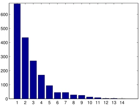
1 2 3 4 5 6 7 8 9 10 11 12 13 14 0 100 200 300 400 500 600

Figure 1: Observed data: number of regions hit by a single event. the return times were previously grouped.

The data are shown in figure 1. They are a subset of the database of the CNR-GNDCI AVI project, developed by the Italian Research Council; de-tails can be found on the web site of the project (see www.avi.gndci.pg.cnr.it and the references therein). The database contains more than 20000 flood events for the whole Italian territory starting from the XVII century; we de-cided to limit ourselves to the events of the period January 1900 - January 2002, which are supposed to be more reliable.

As for the auxiliary variables, we have a list containing mostly physical variables:

• area;

• position (geographical coordinates); • population;

• maximum, minimum and average altitude; • rainfall in 1, 3, 12 and 24 hours;

• dimension of the basin.

The interpretation of the role played by these variables with respect to flood events is sometimes, but not always, easy (we expect a flood event to be more frequent where it falls more rain and where the altitude is larger; on the other hand, the role of position is less clear); as for the single non-physical variable (population), it is more difficult to predict its impact. In any case, the selection of significant variables is likely to require both statistical tools and “expert opinions”.

2.2 The Logistic Auto-Logistic (LAM) model

The specification of the model has to take into account the features listed

above and, in particular, the facts that Yi is a binary variable and that

we are interested in estimating the impact of auxiliary variables on the probability of an event. In order to satisfy both requirements, we adopt a further extension of the standard logistic framework, namely the so-called Logistic Auto-Logistic (LAM) model ([8], pag. 125-126; see [9] for a more general treatment of auto-models). Before giving a formal definition of the model, we need two definitions.

Definition 1 (Neighborhood criterion). A site j is called neighbor of site

i if the distribution of Yi, conditionally on the values of Y in all the other

sites, depends on Yj.

Definition 2 (Neighborhood set). The set C{i} = {j : j is a neighbor of i}

(j = 1, . . . , N ) is called neighbors set of i.

Notice that, from a theoretical point of view, the neighborhood criterion is not necessarily related to geographical adjacency, but is defined by a known matrix C (the connectivity matrix) which identifies the areas belong-ing to C{i} (this is sometimes called contiguity-based neighborhood); roughly speaking, what happens in the areas not belonging to C{i} does not have any influence on the conditional probability of success.

The model can now be formalized writing down explicitly the conditional probability of “success” in area i:

P (Yi = 1|Yj, j 6= i, j ∈ C{i}) =

exp{α + γ′xi+ βP_j∈C{i}yj}

1 + exp{α + γ′_{xi+ β}P

j∈C{i}yj}

. (1) At first glance, model (1) may seem similar to the standard logit model, but from the probabilistic point of view the differences are remarkable.

First, the observations Yi are dependent, because of the presence of the

termP

j∈C{i}yj in the score function, which implies that the probability of

observing a success in region i is influenced by the number of successes in

contiguous regions. Second, the vector xi contains the auxiliary variables

of the i-th area, and α, γ and β are the unknown parameters to be

esti-mated. Formulation (1) and, in particular, the dependence of the Yi’s, has

a relevant impact on estimation: as we will see in the next section, classical Maximum Likelihood Estimation (MLE) is not feasible, and the most con-venient solution consists in using Pseudo Maximum Likelihood Estimation (PMLE), which provides us with estimators which share most of the well known properties of MLE’s and allows to avoid the problems of standard MLE in this setup.

The probabilistic model underlying (1) is a spatial random process or a random field. Referring to [8], chap. 2, for details, we limit ourselves to recall that a random field is an extension of the well known concept of random process: while the latter describes the stochastic evolution over time of a single variable, the random field gives the same information for a family of random vectors. It represents the natural model for our framework, because

Y is a binary vector evolving over time.

So far, we have only specified the conditional distribution of Yi given Yj

(j 6= i). From the theoretical point of view, this introduces a major problem: is it possible to define a functional form for the conditional distribution of each random variable and then derive the joint distribution of the N random variables? In other words, do the univariate conditional distributions contain enough information to fully characterize the joint distribution? The answer to this question is positive under the so-called positivity condition, which requires all the marginal distributions of Y to be strictly positive. This

result was proved by Hammersley and Clifford ([10]) in a famous theorem which circulated for some years in a private form and was subsequently published by other authors ([6], [11], [12]).

Theorem 1 (Hammersley-Clifford). Under the positivity condition, the

joint distribution g of Y satisfies g(y1, . . . , yp) ∝ p Y j=1 glj(ylj|yl1, . . . , yli−1, y ′ li+1, . . . , y ′ lp) glj(yl′_j|yl1, . . . , yli−1, y ′ li+1, . . . , y ′ lp)

for every permutation l on {1, 2, . . . , p} and every y′ _{∈ Y, where Y is the}

sample space of Y .

Proof: see, for example, [13], sect. 7.1.5.

It is easily verified ([7], sect. 2.4.2.4) that both the autologistic model and the LAM model satisfy the positivity condition, so that the Hammersley-Clifford theorem holds in our setup and we can safely estimate the condi-tional distributions and use them to simulate the model.

In applications, model (1) is certainly useful in a conditional setup, in the sense that it gives an estimate of the probability of a flood event in the i-th region given that we know what has happened in the neighborinhg regions. However, this is usually only part of the information needed for practical purposes: both insurance companies and civil protection plans are indeed mostly interested in an “overall” probability of observing a flood event in a certain region, not dependent on the presence of the event in neighboring regions. This unconditional probability can be interpreted as the average riskiness of a region if we ignore what has happened elsewhere: it follows that it is clearly the most important one in the long run, because it can also be thought of as the average riskiness, in the sense that it corresponds to the average of the conditional probabilities as the conditioning events change over time. The latter probability is obviously the risk measure of interest for insurance companies.

It is worth noting that a similar interpretation of risk is common to other fields: in particular, credit risk measurement is interested in both conditional default probabilities (for short run analysis) and unconditional

default probabilities, which give an average riskiness over a longer time horizon.

2.3 The unconditional distribution

The Hammersley-Clifford theorem guarantees the existence and uniqueness

of the joint distribution of the Yi’s, but it does not give its exact form,

and the normalizing constant needed to identify it may be very difficult to compute. As a consequence, finding analytically the unconditional joint distribution of Y is often impossible. To see where the problem comes from in the autologistic model, consider the following well known example ([14], pag. 323; [8], pag. 52-55).

Example 1 (Ising model). From the statistical point of view, the Ising

model of statistical mechanics is a particular version of the autologistic

model. The setup is as follows. A binary variable Yij is defined on a

rect-angular array; two sites (i, j) and (k, s) are neighbors if either i = k and

|j − s| = 1 or j = s and |i − k| = 1. Let S =P P yij be the total

num-ber of successes and nij the sum of yks over the four neighboring sites of

(i, j). Let finally N = (1/2)P P nij. In the Ising model the probability of

a realization y of the random field is given by

P (y) = 1

Z(α, β)exp {αS + βN }. (2)

The normalizing constant Z(α, β) is such that P P P (Yij) = 1; in other

words, it has to be introduced in order to make (2) a probability distribution. Unfortunately, this quantity is computationally intractable, so that the joint distribution cannot be determined.

On the other hand, the conditional probabilities of Yij given all the other

y’s take a simple form:

P (Yij = 1|all other y’s) =

exp {α + βnij}

1 + exp {α + βnij}

.

Although the Hammersley-Clifford theorem is not useful for the compu-tation of the joint distribution, it guarantees its existence, giving a sound

foundation to the common practice of using the conditional probabilities in applications. In the following we will indeed see that estimation can be performed by means of (1) and that the joint distribution can be obtained numerically, via the Gibbs Sampling algorithm, using again the conditional distributions (1).

3

Estimation and simulation: a MCMC Approach

In the preceding section we have recalled that the Hammersley-Clifford the-orem does not allow to find exactly the joint distribution of the random field

Y. For estimation purposes, this is a serious problem.

Example 1 (continued). We pointed out in the preceding section that the

normalization constant Z(α, β) is not computable; moreover, it depends on the unknown parameters α and β, so that we cannot drop it when we write down the likelihood function. The conclusion is that standard MLE of α and β cannot be performed if we start from the joint distribution (2).

3.1 Maximum Pseudo-Likelihood Estimation

The conditional distributions in the autologistic model take a very simple form because, if we consider the joint distribution and apply the definition to find the conditional distributions, the normalization constant drops down (see [15]). This feature, combined with the difficulties associated to stan-dard MLE, led researchers to develop an estimation theory based on the conditional distributions.

In particular, Besag ([17], [18]) was the first to introduce a methodology called Pseudo-Maximum Likelihood Estimation (PMLE). The basic idea is simple: according to classical MLE, if the observations are dependent we cannot compute the likelihood function for all the variables by simply taking the product of the conditional distributions of each observations given all the other observations. To apply PMLE, we ignore this problem and compute the function

as if the observations were conditionally independent. Of course (3) is not a likelihood function, and for this reason it is called Pseudo-Maximum Likeli-hood.

Given that one of the main hypotheses of maximum likelihood estima-tion is violated, we expect that the properties of MLE’s do not extend to this setup, but fortunately most of these properties continue to hold true. In par-ticular, under standard regularity conditions, [19] have shown that PMLE’s are consistent and asymptotically normal, with asymptotic variances given by quantities whose interpretation is similar to the elements of the inverse of the Fisher information matrix in classical MLE (see, for example, [20], sect. 9.2).

Essentially, as pointed out by [14], the only property not inherited by PMLE’s is efficiency. However, inefficiency is usually small, and compen-sated by huge computational advantages; using Cressie’s words ([9], pag. 461), the pseudo-maximum likelihood procedures “trade away efficiency in exchange for closed-form expressions that avoid working with the exact like-lihood’s unwieldy normalizing constant”. In our setup, the application of PMLE to (1) is straightforward: we employ standard maximum likelihood techniques for the estimation of the parameters of the logit model.

3.2 The simulation of the joint distribution

Having estimated the parameters of (1) by means of PML techniques, the

next step consists in finding the joint distribution of the Yi’s. This

prob-lem cannot be solved analytically, so that we have to resort to simulation techniques. Considering that we know the univariate conditional probabil-ity distributions, it is natural to use the Gibbs sampling algorithm for the determination of the joint distribution.

The Gibbs sampler ([21]; see [13] for a general treatment and [22] for a more application-oriented analysis) is an algorithm which allows to simu-late the joint distribution of p random variables using only the p univariate conditional distributions.

Definition 3 (Gibbs Sampler). Let Y = (Y1, . . . , Yp)′ be a p-variate

conditional densities fi, namely

Yi|y1, y2, . . . , yi−1, yi−1, . . . , yp ∼ fi(yi|y1, y2, . . . , yi−1, yi−1, . . . , yp)

for i = 1, . . . , p. Then the Gibbs Sampler is given by the following steps:

given the values (y₁(t), . . . , yp(t)) obtained at the t-th iteration, simulate

1. Y₁(t+1) ∼ f1(y1|y₂(t), . . . , yp(t)); 2. Y₂(t+1) ∼ f2(y2|y1(t+1), y (t) 3 , . . . , y (t) p ); .. . p. Yp(t+1) ∼ fp(yp|y₁(t+1), . . . , y(t+1)_p−1 ).

The application of the algorithm to our setup is rather straightforward: all we need are the univariate conditional densities, which are given by (1). Thus, the t-th replication of the algorithm consists in simulating p Bernoulli

random variables Y_i(t) with parameters ˆπ(t)_i (i = 1, . . . , p), where ˆπ(t)_i is given

by: ˆ π(t)_i = exp{ ˆα+ ˆγ ′_x i+ ˆβP_j∈C{i}yj(t−1)} 1 + exp{ ˆα+ ˆγ′xi+ ˆβP_j∈C{i}y(t−1)j } .

The crucial feature of the algorithm ([13], chap. 7) is that each sequence of random variables generated by the Gibbs Sampler is an ergodic Markov chain whose stationary distribution is the joint distribution of the p variables; nonetheless, this result is of little use for practical purposes, because it does not tell us when convergence is reached. Thus, the last important issue in applications is the determination of a stopping criterion.

Diagnosing convergence has always proved to be a difficult problem. Unfortunately, no general recipe is available, as the convergence behavior of the chain depends on the setting; in other words, it is problem-specific. Referring the reader to [13], chap. 8, for details, here we limit ourselves to mention the classical criterion consisting in simulating B independent chains and discarding the “initial” observations (corresponding to the so-called burn-in period) of every chain; if correctly implemented, it is still one of the most reliable criteria. The idea of simulating B independent chains seems to be a sound solution to the problem that adjacent observations of

a single chain are dependent, which implies that, when an iid sample is needed, including contiguous observations is incorrect. After simulating B chains, an iid sample is obtained by taking the “final” observations of each chain.

4

Application

4.1 Estimation of the conditional distributions

According to section 3.1, the first step of the estimation procedure consists in estimating the parameters α, β and γ in (1) by means of the Pseudo-Maximum Likelihood methodology. This means that we treat the obser-vations as if they were independent and use standard maximum likelihood procedures.

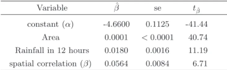
The results are shown in table 1. The auxiliary variables used in the analysis have been obtained by means of a selection procedure performed on a larger set of variables: in particular, the original dataset contained the average rainfall (measured as the average of the yearly maximum rainfall in a given time) for 1, 3, 6, 12, 24 hours, but the only significant one was the 12-hour average.

Table 1. Estimated coefficients, standard errors and t-statistics

Variable βˆ se tβˆ

constant (α) -4.6600 0.1125 -41.44 Area 0.0001 <0.0001 40.74 Rainfall in 12 hours 0.0180 0.0016 11.19 spatial correlation (β) 0.0564 0.0084 6.71

As pointed out by [15], we cannot apply standard distributional results, so that the t statistics should only be considered an informal basis for model selection. However, roughly speaking, we believe that in this case they are reliable for at least two reasons:

• the small value of ˆβ implies that the dependence of the Yi’s is weak, so

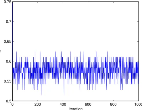
0 200 400 600 800 1000 0.5 0.55 0.6 0.65 0.7 0.75 Iteration π

Figure 2: A typical simulated chain. inappropriate;

• the p-values of the t-statistics are very small, therefore they provide us with a very clear-cut indication about the significance of the variables.

4.2 Simulating the joint distribution

The estimation of the univariate conditional distributions constitutes a nec-essary step for the implementation of the Gibbs Sampler, because the sim-ulation is based on the univariate conditional distributions with parameters

ˆ

α, ˆβ and ˆγ. The application of the Gibbs Sampler follows closely definition

3.

As for the issue of diagnosing convergence, monitoring the sequences {ˆπ_i(j)}j=1,2,... (i = 1, . . . , N ) we noticed that, for any starting value and for

any region, the chain immediately moves in a well defined interval (see figure 2).

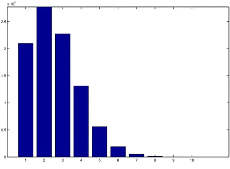
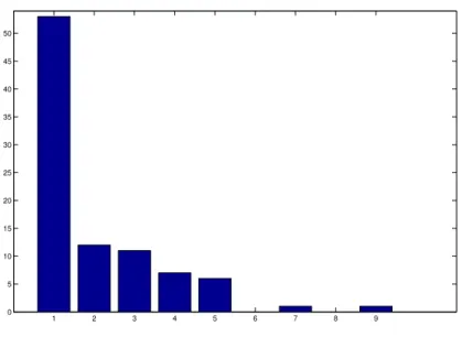
1 2 3 4 5 6 7 8 9 10 0 0.5 1 1.5 2 2.5 x 104

Figure 3: Simulated data: number of regions hit by a single event. Thus we decided to simulate, for each region, a single chain of length T =

1000 and take the average of the last 100 observations ˆπi = (1/100)P1000_t=901πˆ_i(t)

as an estimate of π_i(t). The fact that convergence is relatively fast is

proba-bly related to the small spatial correlation of the areas under investigation

as measured by the numerical value of ˆβ.

The final values of the chains obtained in a single replication of the algorithm form an observation from the joint (N -variate) distribution of the

Yi’s. Given the binary nature of the variables of interest, each simulated

observation is a vector y∗ ∈ {0, 1}N_{. Simulating B = 100, 000 observations}

and computing W∗

k =

PN

i=1yi∗(k = 1, . . . , N ), we get the distribution shown

in figure 3.

The graph gives the frequency distribution of the number of areas hit by a flood event, and can therefore be interpreted as a measure of its spatial extension; this information is clearly important both for civil protection purposes and for insurance companies, because, in absence of a ranking of the severity of floodings, it can be taken as the most basic measure of the gravity of an event.

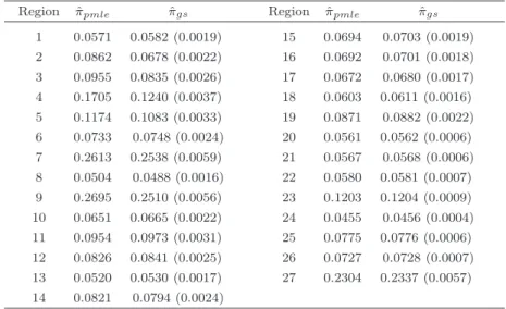
Estimated values ˆπGS of π are given in table 2 along with standard

errors. For comparison purposes, we also reported the probabilities ˆπP M LE

obtained by means of the univariate logistic regressions estimated in the preceding section.

Table 2. Parameter estimates and standard errors obtained by means

of univariate PMLE (ˆπP M LE) and Gibbs Sampler (ˆπGS)

Region ˆπpmle πˆgs Region πˆpmle ˆπgs

1 0.0571 0.0582 (0.0019) 15 0.0694 0.0703 (0.0019) 2 0.0862 0.0678 (0.0022) 16 0.0692 0.0701 (0.0018) 3 0.0955 0.0835 (0.0026) 17 0.0672 0.0680 (0.0017) 4 0.1705 0.1240 (0.0037) 18 0.0603 0.0611 (0.0016) 5 0.1174 0.1083 (0.0033) 19 0.0871 0.0882 (0.0022) 6 0.0733 0.0748 (0.0024) 20 0.0561 0.0562 (0.0006) 7 0.2613 0.2538 (0.0059) 21 0.0567 0.0568 (0.0006) 8 0.0504 0.0488 (0.0016) 22 0.0580 0.0581 (0.0007) 9 0.2695 0.2510 (0.0056) 23 0.1203 0.1204 (0.0009) 10 0.0651 0.0665 (0.0022) 24 0.0455 0.0456 (0.0004) 11 0.0954 0.0973 (0.0031) 25 0.0775 0.0776 (0.0006) 12 0.0826 0.0841 (0.0025) 26 0.0727 0.0728 (0.0007) 13 0.0520 0.0530 (0.0017) 27 0.2304 0.2337 (0.0057) 14 0.0821 0.0794 (0.0024)

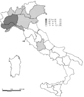
The differences between the flooding probabilities computed with the two methods are displayed graphically in figure 4.

The map shows that the difference between the univariate and the joint estimates are mostly small; the most relevant exception is given by region 4,

for which ˆπP M LEis significantly larger than ˆπGS. It is difficult to identify the

causes of this outcome: we checked the values of the auxiliary variables, and they are similar to the values observed in other regions. Thus, the difference must be related to the spatial autocorrelation between the regions, and this difference underlines the importance of estimating the probability of flood events on the basis of the joint distribution.

Figure 4: Differences between univariate and joint estimates.

5

Risk Assessment

It is intuitively clear that not all floodings cause the same damages, and this is obviously important. Thus, in order to give a more precise description of the associated risk, we need to introduce some measure of the severity of the events.

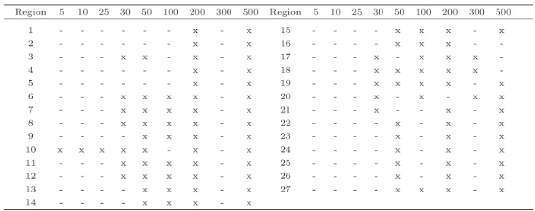
In the application at hand, times of return based on expert opinions are available; in Extreme Value Theory, times of return are a common way of describing the severity of events (see [4]), because there is a monotonically increasing function relating the severity of an event to its time of return.

Table 3. Times of return in years Region 5 10 25 30 50 100 200 300 500 Region 5 10 25 30 50 100 200 300 500 1 - - - x - x 15 - - - - x x x - x 2 - - - x - x 16 - - - - x x x - -3 - - - x x - x - x 17 - - - x - x x x -4 - - - x - x 18 - - - x x x x x -5 - - - x - x 19 - - - x x x x - x 6 - - - x x x x - x 20 - - - x - x - x x 7 - - - x x x x - x 21 - - - x - - x - x 8 - - - x x x x - x 22 - - - - x - x - x 9 - - - - x x x - x 23 - - - - x - x - x 10 x x x x x - x - x 24 - - - - x - x - x 11 - - - x x x x - x 25 - - - - x - x - x 12 - - - x x x x - x 26 - - - - x - x - x 13 - - - - x x x - x 27 - - - - x x x - x 14 - - - - x x x - x

Unfortunately, we do not have any probabilistic measure about the times of return, whose interpretation is as follows: the symbol × in the table means that the flood event affecting that region has the time of return corresponding to the column. For example, floodings which impact region 1 have a time of return equal to either 200 or 500 years. The only way of associating a probability to the symbols in the table consists in introducing the following two assumptions:

(i) the severity of events is a linear function of the times of return and is labelled from 1 (lightest event, corresponding to a 5 years time of return) to 9 (strongest event, corresponding to a 500 years time of return).

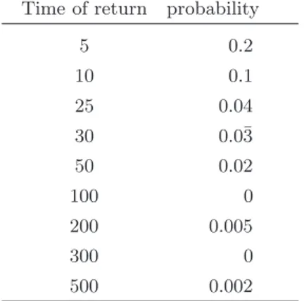
(ii) as a “light” event is supposed to occur more frequently than a “strong” event, the probability of a certain time of return is negatively related to its severity. In particular, we decided to compute the probability of the j-th time of return for the i-th region as follows:

qij =

 



1/tj if the j-th time of return occurs in the i-th area,

0 else,

where tj is the j-th time of return. Obviously, we then have to

ize these probabilities so that their sum is equal to one; after

normal-ization, we call these probabilities pij. As an example, probabilities of

Table 4. Probabilities of times of return for region 10

Time of return probability

5 0.2 10 0.1 25 0.04 30 0.0¯3 50 0.02 100 0 200 0.005 300 0 500 0.002

The simulation then proceeds according to the probabilities of the times

of return pij. Defining Si to be a discrete random variable taking values

in {1, . . . , 9} with probabilities pi1, . . . , pi9, for each region we perform the

following steps:

1. find the flood events (i.e., find the values y∗

ij = 1, j = 1, . . . , B) in the

simulated vectors y∗₁, . . . , y∗_B;

2. for each y∗_ij = 1, simulate a random number s∗_i from the discrete

distribution of Si and substitute s∗i to y∗ij.

The new vector y∗_j is such that the frequency of flood events is the same as in

the first part of the simulation, but now the events have different severities, according to the estimated times of return. As an example, figure 5 shows the distribution of the severities of the events simulated for area 10.

5.1 Introducing spatial autocorrelation

From section 4 (see table 1) we know that the estimated numerical value of the autocorrelation parameter β is rather small, so that the autocorrelation of the events simulated from the joint distribution is small as well. The value

of ˆβ is undoubtedly related to the specification of the contiguity matrix C: in

particular, such a result is likely to be determined by the fact that C contains “many” zeros or, in other words, each region has few neighbors. From the practitioners’ point of view, underestimating spatial dependence can be

1 2 3 4 5 6 7 8 9 0 5 10 15 20 25 30 35 40 45 50

Figure 5: Severity of the simulated events for area 10.

dangerous, as it would imply an underrate of the total risk as measured by means of the joint distribution.

A possible remedy consists in increasing spatial autocorrelation ex post; to this aim, we propose to use an algorithm which “switches” the simulated events in order to increase spatial autocorrelation as measured by the Moran index (see [16] for a thorough description):

I = P N i P jcij P i P jcij(yi∗− ¯y∗)(yj∗− ¯y∗) P i(yi∗− ¯y∗)2 .

More precisely, the k-th iteration of the algorithm, which resembles the spin-exchange algorithm ([23]; [24]; [9], pag. 572), is based on the following steps:

(i) two replications of the simulation (that is, two N -dimensional vectors

y∗_i and y∗_j) are chosen at random;

(ii) if at least one component y∗

ij and y∗sj is non-zero in both vectors and

has different severity, sum the values of the Moran index computed on

the two replications; call M1 the value obtained;

(iii) switch the events y_ij∗ and y_sj∗ and recompute the Moran index; call M2

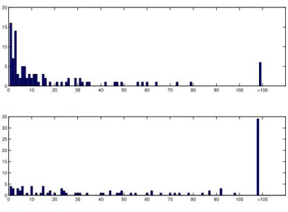
0 10 20 30 40 50 60 70 80 90 100 >100 0 5 10 15 20 0 10 20 30 40 50 60 70 80 90 100 >100 0 5 10 15 20 25 30 35

Figure 6: Iterations needed for a 10% (top) and 20% (bottom) increase.

(iv) if M2 > M1, start a new iteration; else, undo the switch and go back

to step (i).

When should we stop the algorithm? We have to decide a priori the amount of spatial autocorrelation we want to add, and then stop the

algo-rithm at the smallest t such that the quantity M(t)_{− M}(1) _{is larger than a}

predefined value ǫ.

To determine the effectiveness of the algorithm, we performed some nu-merical experiments. We ran it 100 times and kept track of the number of iterations needed to increase the spatial autocorrelation of the simulated events by a percentage of ǫ%, with values of ǫ equal respectively to 10% and 20%. Figure 6 gives the results.

6

Conclusions

In this paper we have proposed a multivariate model for the estimation and simulation of flood events. The model allows to incorporate two essential requirements: the inclusion of additional information possibly contained in auxiliary variables and the explicit consideration of spatial autocorrelation.

The simulation procedure accounts for the severity of events, according to times of return estimated by means of expert opinions. Although spatial dependence is explicitly considered by the model, it may be appropriate to modify ex post the results in order to get a larger spatial autocorrelation without changing the marginal probability distributions of the events in each area; to this aim, we developed an algorithm, based on a methodology similar to the spin-exchange, for increasing the spatial dependence of the simulated events.

Although this model constitutes an improvement with respect to more standard approaches used in this field, many problems remain open. In par-ticular, we stress the necessity of introducing a more precise estimate of the severity of events, which is strictly related to the availability of more accu-rate data concerning either the times of return or other auxiliary variables carrying some information about the “magnitude” of observed floodings. Another issue that should be explored more thoroughly concerns the use of the algorithm which increases ex post the spatial autocorrelation of the simulated events: some criterion about the amount of the increase should indeed be established.

References

[1] Mikosch T. Non-Life Insurance Mathematics. Springer: New York, 2004.

[2] Jewson S, Brix A, Ziehmann C. Weather Derivative Valuation: The Meteorological, Statistical, Financial and Mathematical Foundations. Cambridge: Cambridge University Press, 2005.

[3] Natural Environment Research Council. Flood Studies Report, 5 Vol-umes. Whitefriars Press: London, 1975.

[4] Embrechts P, Kluppelberg C, Mikosch T. Modelling Extremal Events for Insurance and Finance. Springer: New York, 1997.

[5] Besag J. Nearest-neighbour systems and the auto-logistic model for binary data. Journal of the Royal Statistical Society B 1972; 34: 76-83.

[6] Besag J. Spatial interaction and the statistical analysis of lattice sys-tems (with discussion). Journal of the Royal Statistical Society B 1974; 36, 192-236.

[7] Arbia G, Espa G. Forecasting statistical models of archaeological site location. Archeologia e Calcolatori 1996; 7: 365-372.

[8] Arbia G. Spatial Econometrics: Statistical Foundations and Applica-tions to regional Convergence. Springer: New York, 2006.

[9] Cressie NAC. Statistics for Spatial Data, revised edition. Wiley: New York, 1993.

[10] Hammersley JM, Clifford P. Markov fields on finite graphs lattices. Unpublished manuscript, 1971.

[11] Preston CJ. Generalized Gibbs states and Markov random fields. Ad-vances in Applied Probability 1973; 5: 242-261.

[12] Grimmett GR. A theorem about random fields, Bulletin of the London Mathematical Society 1973; 79: 5.

[13] Casella G, Robert CP. Monte Carlo Statistical Methods. Springer: New York, 1999.

[14] Strauss D. The Many Faces of Logistic Regression. The American Statistician 1992; 46: 321-327.

[15] Strauss D, Ikeda M. Pseudolikelihood estimation for social networks. Journal of the American Statistical Association 1990; 85: 204-212. [16] Cliff AD, Ord JK. Spatial Processes. Models and Applications. Pion:

London, 1981.

[17] Besag J. Statistical analysis of non-lattice data, The Statistician 1975; 24, 179-195.

[18] Besag J. Efficiency of pseudo-likelihood estimators for simple Gaussian fields Biometrika 1977; 64, 616-618.

[19] Arnold BC, Strauss D. Pseudo likelihood estimation: some examples. Sankhya B 1991; 53, 233-243.

[20] Cox DR, Hinkley DV. Theoretical Statistics. Chapman and Hall: Lon-don, 1974.

[21] Geman S, Geman D. Stochastic relaxation, Gibbs distributions, and the Bayesian restoration of images, IEEE Transactions on Pattern Analysis and Machine Intelligence 1984; 6, 721-741.

[22] Gilks WR, Richardson S, Spiegelhalter DJ. (eds) Markov Chain Monte Carlo in Practice. Chapman and Hall: London, 1996.

[23] Flinn PA. Monte Carlo calculation of phase separation in a two-dimensional Ising system. Journal of Statistical Physics 1974; 10, 89-97. [24] Cross GR, Jain AK. Markov random field texture models. IEEE Trans-actions on Pattern Analysis and Machine Intelligence 1983; PAMI-5, 25-39.

Elenco dei papers del Dipartimento di Economia

2000.1 A two-sector model of the effects of wage compression on unemployment and industry distribution of employment, by Luigi Bonatti 2000.2 From Kuwait to Kosovo: What have we learned? Reflections on globalization and peace, by Roberto Tamborini

2000.3 Metodo e valutazione in economia. Dall’apriorismo a Friedman , by Matteo Motterlini

2000.4 Under tertiarisation and unemployment. by Maurizio Pugno 2001.1 Growth and Monetary Rules in a Model with Competitive Labor Markets, by Luigi Bonatti.

2001.2 Profit Versus Non-Profit Firms in the Service Sector: an Analysis of the Employment and Welfare Implications, by Luigi Bonatti, Carlo Borzaga and Luigi Mittone.

2001.3 Statistical Economic Approach to Mixed Stock-Flows Dynamic Models in Macroeconomics, by Bernardo Maggi and Giuseppe Espa. 2001.4 The monetary transmission mechanism in Italy: The credit channel and a missing ring, by Riccardo Fiorentini and Roberto Tamborini. 2001.5 Vat evasion: an experimental approach, by Luigi Mittone

2001.6 Decomposability and Modularity of Economic Interactions, by Luigi Marengo, Corrado Pasquali and Marco Valente.

2001.7 Unbalanced Growth and Women’s Homework, by Maurizio Pugno 2002.1 The Underground Economy and the Underdevelopment Trap, by Maria Rosaria Carillo and Maurizio Pugno.

2002.2 Interregional Income Redistribution and Convergence in a Model with Perfect Capital Mobility and Unionized Labor Markets, by Luigi Bonatti.

2002.3 Firms’ bankruptcy and turnover in a macroeconomy, by Marco Bee, Giuseppe Espa and Roberto Tamborini.

2002.4 One “monetary giant” with many “fiscal dwarfs”: the efficiency of macroeconomic stabilization policies in the European Monetary Union, by Roberto Tamborini.

2002.5 The Boom that never was? Latin American Loans in London 1822-1825, by Giorgio Fodor.

2002.6 L’economia senza banditore di Axel Leijonhufvud: le ‘forze oscure del tempo e dell’ignoranza’ e la complessità del coordinamento, by Elisabetta De Antoni.

2002.7 Why is Trade between the European Union and the Transition

Economies Vertical?, by Hubert Gabrisch and Maria Luigia Segnana. 2003.1 The service paradox and endogenous economic gorwth, by Maurizio Pugno.

2003.2 Mappe di probabilità di sito archeologico: un passo avanti, di Giuseppe Espa, Roberto Benedetti, Anna De Meo e Salvatore Espa. (Probability maps of archaeological site location: one step beyond, by Giuseppe Espa, Roberto Benedetti, Anna De Meo and Salvatore Espa). 2003.3 The Long Swings in Economic Understianding, by Axel Leijonhufvud.

2003.4 Dinamica strutturale e occupazione nei servizi, di Giulia Felice. 2003.5 The Desirable Organizational Structure for Evolutionary Firms in Static Landscapes, by Nicolás Garrido.

2003.6 The Financial Markets and Wealth Effects on Consumption An Experimental Analysis, by Matteo Ploner.

2003.7 Essays on Computable Economics, Methodology and the Philosophy of Science, by Kumaraswamy Velupillai.

2003.8 Economics and the Complexity Vision: Chimerical Partners or Elysian Adventurers?, by Kumaraswamy Velupillai.

2003.9 Contratto d’area cooperativo contro il rischio sistemico di produzione in agricoltura, di Luciano Pilati e Vasco Boatto.

2003.10 Il contratto della docenza universitaria. Un problema multi-tasking, di Roberto Tamborini.

2004.1 Razionalità e motivazioni affettive: nuove idee dalla neurobiologia e psichiatria per la teoria economica? di Maurizio Pugno.

(Rationality and affective motivations: new ideas from neurobiology and psychiatry for economic theory? by Maurizio Pugno.

2004.2 The economic consequences of Mr. G. W. Bush’s foreign policy. Can th US afford it? by Roberto Tamborini

2004.3 Fighting Poverty as a Worldwide Goal by Rubens Ricupero

2004.4 Commodity Prices and Debt Sustainability by Christopher L. Gilbert and Alexandra Tabova

2004.5 A Primer on the Tools and Concepts of Computable Economics by K. Vela Velupillai

2004.6 The Unreasonable Ineffectiveness of Mathematics in Economics by Vela K. Velupillai

2004.7 Hicksian Visions and Vignettes on (Non-Linear) Trade Cycle Theories by Vela K. Velupillai

2004.8 Trade, inequality and pro-poor growth: Two perspectives, one message? By Gabriella Berloffa and Maria Luigia Segnana

2004.9 Worker involvement in entrepreneurial nonprofit organizations. Toward a new assessment of workers? Perceived satisfaction and fairness by Carlo Borzaga and Ermanno Tortia.

2004.10 A Social Contract Account for CSR as Extended Model of Corporate Governance (Part I): Rational Bargaining and Justification by Lorenzo Sacconi

2004.11 A Social Contract Account for CSR as Extended Model of Corporate Governance (Part II): Compliance, Reputation and Reciprocity by Lorenzo Sacconi

2004.12 A Fuzzy Logic and Default Reasoning Model of Social Norm and Equilibrium Selection in Games under Unforeseen Contingencies by Lorenzo Sacconi and Stefano Moretti

2004.13 The Constitution of the Not-For-Profit Organisation: Reciprocal Conformity to Morality by Gianluca Grimalda and Lorenzo Sacconi 2005.1 The happiness paradox: a formal explanation from psycho-economics by Maurizio Pugno

2005.2 Euro Bonds: in Search of Financial Spillovers by Stefano Schiavo 2005.3 On Maximum Likelihood Estimation of Operational Loss Distributions by Marco Bee

2005.4 An enclave-led model growth: the structural problem of informality persistence in Latin America by Mario Cimoli, Annalisa Primi and Maurizio Pugno

2005.5 A tree-based approach to forming strata in multipurpose business surveys, Roberto Benedetti, Giuseppe Espa and Giovanni Lafratta. 2005.6 Price Discovery in the Aluminium Market by Isabel Figuerola-Ferretti and Christopher L. Gilbert.

2005.7 How is Futures Trading Affected by the Move to a Computerized Trading System? Lessons from the LIFFE FTSE 100 Contract by

2005.8 Can We Link Concessional Debt Service to Commodity Prices? By Christopher L. Gilbert and Alexandra Tabova

2005.9 On the feasibility and desirability of GDP-indexed concessional lending by Alexandra Tabova.

2005.10 Un modello finanziario di breve periodo per il settore statale italiano: l’analisi relativa al contesto pre-unione monetaria by Bernardo Maggi e Giuseppe Espa.

2005.11 Why does money matter? A structural analysis of monetary policy, credit and aggregate supply effects in Italy, Giuliana Passamani and Roberto Tamborini.

2005.12 Conformity and Reciprocity in the “Exclusion Game”: an Experimental Investigation by Lorenzo Sacconi and Marco Faillo. 2005.13 The Foundations of Computable General Equilibrium Theory, by K. Vela Velupillai.

2005.14 The Impossibility of an Effective Theory of Policy in a Complex Economy, by K. Vela Velupillai.

2005.15 Morishima’s Nonlinear Model of the Cycle: Simplifications and Generalizations, by K. Vela Velupillai.

2005.16 Using and Producing Ideas in Computable Endogenous Growth, by K. Vela Velupillai.

2005.17 From Planning to Mature: on the Determinants of Open Source Take Off by Stefano Comino, Fabio M. Manenti and Maria Laura Parisi.

2005.18 Capabilities, the self, and well-being: a research in psycho-economics, by Maurizio Pugno.

2005.19 Fiscal and monetary policy, unfortunate events, and the SGP arithmetics. Evidence from a growth-gap model, by Edoardo Gaffeo, Giuliana Passamani and Roberto Tamborini

2005.20 Semiparametric Evidence on the Long-Run Effects of Inflation on Growth, by Andrea Vaona and Stefano Schiavo.

2006.1 On the role of public policies supporting Free/Open Source Software. An European perspective, by Stefano Comino, Fabio M. Manenti and Alessandro Rossi.

2006.2 Back to Wicksell? In search of the foundations of practical monetary policy, by Roberto Tamborini

2006.4 Worker Satisfaction and Perceived Fairness: Result of a Survey in Public, and Non-profit Organizations, by Ermanno Tortia

2006.5 Value Chain Analysis and Market Power in Commodity Processing with Application to the Cocoa and Coffee Sectors, by Christopher L. Gilbert 2006.6 Macroeconomic Fluctuations and the Firms’ Rate of Growth Distribution: Evidence from UK and US Quoted Companies, by Emiliano Santoro

2006.7 Heterogeneity and Learning in Inflation Expectation Formation: An Empirical Assessment, by Damjan Pfajfar and Emiliano Santoro

2006.8 Good Law & Economics needs suitable microeconomic models: the case against the application of standard agency models: the case against the application of standard agency models to the professions, by Lorenzo Sacconi

2006.9 Monetary policy through the “credit-cost channel”. Italy and Germany, by Giuliana Passamani and Roberto Tamborini

2007.1 The Asymptotic Loss Distribution in a Fat-Tailed Factor Model of Portfolio Credit Risk, by Marco Bee

2007.2 Sraffa?s Mathematical Economics – A Constructive Interpretation, by Kumaraswamy Velupillai

2007.3 Variations on the Theme of Conning in Mathematical Economics, by Kumaraswamy Velupillai

2007.4 Norm Compliance: the Contribution of Behavioral Economics Models, by Marco Faillo and Lorenzo Sacconi

2007.5 A class of spatial econometric methods in the empirical analysis of clusters of firms in the space, by Giuseppe Arbia, Giuseppe Espa e Danny Quah.

2007.6 Rescuing the LM (and the money market) in a modern Macro course, by Roberto Tamborini.

2007.7 Family, Partnerships, and Network: Reflections on the Strategies of the Salvadori Firm of Trento, by Cinzia Lorandini.

2007.8 I Verleger serici trentino-tirolesi nei rapporti tra Nord e Sud: un approccio prosopografico, by Cinzia Lorandini.

2007.9 A Framework for Cut-off Sampling in Business Survey Design, by Marco Bee, Roberto Benedetti e Giuseppe Espa