Energy Methods for Fracture and Fatigue Assessment

(1)

D

EPARTMENT OF

E

NGINEERING

PHD.COURSE IN ENGINEERING AND CHEMISTRY OF MATERIALS AND CONSTRUCTIONS XXXIIICYCLE

E

NERGY

M

ETHODS FOR

F

RACTURE AND

F

ATIGUE ASSESSMENT

Dario Francesco Santonocito

Tutor: Prof. Giacomo Risitano

SSD: ING/IND-14 – Progettazione meccanica e costruzione di macchine

(2)

i

S

UMMARY

The present Ph.D. thesis is the collection of three years of research activity in the fatigue field. The aim of the thesis was to apply Energy based methods to the assessment of the fatigue properties of materials.

The Risitano Thermographic Method and the novel Static Thermographic Method were extensively applied to a wide set of materials in order to validate them as rapid test procedures able to derive, in short amount of time and with few specimens, the fatigue properties of materials monitoring the energetic release.

Finite element simulations were carried out to applying the Strain Energy Density method as a local approach to predict the fatigue failure of notched mechanical components.

The Thermographic Method-s were applied to structural steel from an in-service component, plain and notched medium carbon steel specimens, high strength concrete under compressive loads, high density polyethylene for pressure pipe applications, 3D printed polyamide-12 specimens and short glass fiber reinforced composite PA66GF35.

The Strain Energy Density approach was applied to welded components, in particular cruciform welded joints, to compare the fatigue information provided by this method with the ones provided by the international welding standards.

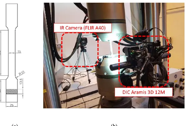
The experimental activities were performed at the Laboratory of Mechanics of the University of Messina. Part of the research period was spent by the author at the University of Padova, under the supervision of Prof. Giovanni Meneghetti, and at the Norwegian University of Science and Technology (NTNU), under the supervision of Prof. Filippo Berto, to study local approaches techniques.

Several research perspectives have been opened by this thesis, that the author would to pursue in the future.

(3)

(4)

iii

T

ABLE OF

C

ONTENTS

Introduction ... x

PART I Theoretical Background 1. Energy dissipation in fatigue test ... 1

1.1. Fatigue in materials ... 2

1.1.1. Fatigue regimes ... 2

1.1.2. Mean stress effect ... 4

1.1.3. Load history ... 5

1.1.4. Stress state ... 6

1.1.5. Some consideration about the test time ... 6

1.2. From microstructure to macroscopic dissipative effect in fatigue ... 7

1.2.1. Temperature trend during a fatigue test ... 8

1.3. Risitano Thermographic Method ... 10

1.4. Energy based approach ... 14

2. Energetic release in static tensile test ... 18

2.1. Stress-Strain-temperature constitutive relationship ... 19

2.1.1. First stress invariant and first strain invariant ... 20

(5)

iv

2.2.1. Isotropic material ... 27

2.2.2. Orthotropic material ... 30

2.3. Thermal behavior under static tensile test ... 32

2.3.1. Early study of the change in the temperature trend during tensile test... 32

2.3.2. Correlation between the energetic release and the material microstructure . 33 2.4. The Static Thermographic Method ... 38

2.4.1. Simplified model of surface temperature of a static tensile test ... 41

2.4.2. Numerical model for predicting the temperature trend from FE analysis .... 44

3. Local Approaches ... 47

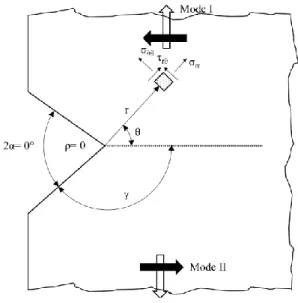
3.1. Linear Elastic Fracture Mechanics for sharp V-Notches ... 48

3.2. Strain Energy Density approach ... 52

3.2.1. Blunt notches ... 59

3.2.2. Fatigue assessment by SED ... 60

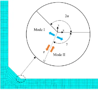
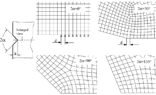
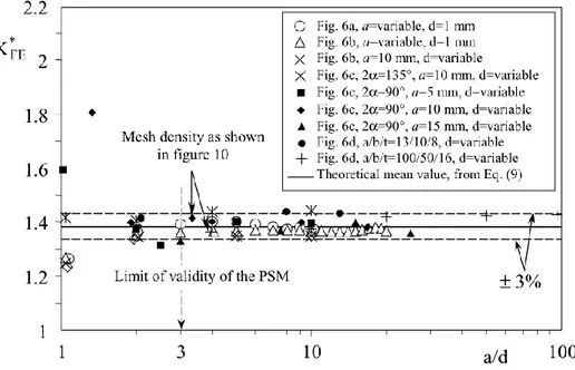
3.3. Peak Stress Method ... 62

3.3.1. PSM for welded joint ... 64

PART II Experimental activities 4. Structural Steel S355 ... 68

Highlights ... 68

Nomenclature ... 68

(6)

v

4.2. Materials and methods... 71

4.3. Results and Discussions ... 73

4.3.1. Material properties... 73

4.3.2. Fatigue tests and Thermographic Method ... 75

4.3.3. Static Thermographic Method... 81

4.4. Conclusion ... 83

5. Medium carbon steel C45 ... 84

Highlights ... 84

Nomenclature ... 84

5.1. Introduction... 85

5.2. Materials and Methods ... 86

5.2.1. Experimental tests ... 86

5.2.2. Numerical simulation ... 87

5.3. Results and Discussion ... 89

5.3.1. Static tensile tests ... 89

5.3.2. Numerical analysis ... 91

5.3.3. Stepwise fatigue test ... 93

5.3.4. Comparison with other test ... 95

6. V-notched medium carbon steel AISI 1035 ... 98

(7)

vi

6.3. Results and discussion ... 104

6.3.1. Fatigue tests ... 104

6.3.2. Energetic release during tensile tests ... 107

6.3.3. Prediction of the temperature trend ... 110

7. High Strength Concrete ... 114

Highlights ... 114

Nomenclature ... 114

7.3. Results and analysis ... 122

8. High-Density Polyethylene ... 131

Highlights ... 131

(8)

vii

8.3.1. Static tensile tests ... 135

8.3.2. Fatigue tests ... 137 8.4. Conclusion ... 141 9. 3D-Printed Polyamide-12 ... 142 Highlights ... 142 Nomenclature ... 142 9.1. Introduction... 143

9.3. Results and discussions ... 146

9.3.1. Mechanical properties ... 146

9.3.2. Static Thermographic Method and Fatigue Limit ... 147

9.3.3. Fracture surfaces... 149

10. Composite material PA66GF35 ... 152

Highlights ... 152

10.1. Introduction ... 153

10.2. Materials and Methods... 154

10.3.1. Experimental test ... 158

(9)

viii

11. Local approaches for welded structures ... 163

Highlights ... 163

11.2. Materials and Methods... 164

12. Fatigue assessment of welded joint by means of SED approach and comparison with standards ... 174

Highlights ... 174

12.2. Fatigue assessment of Cruciform and T-joint by Standards ... 179

12.2.1. Fatigue assessment by Eurocode 3 ... 180

12.2.2. Fatigue assessment by British Standard and International Institute of Welding 182 12.2.3. Fatigue assessment by DNV-GL ... 184

12.3. Finite elements modelling ... 186

(10)

ix

12.4.2. Scale effect ... 192

12.4.3. Full, partial and incomplete penetration ... 194

12.4.4. Welding Bead Height ... 197

12.4.5. Comparison between the Standards and the SED Method ... 197

Concluding remarks ... 200

List of pubblications ... 202

Acknowledgments ... 204

(11)

x

I

NTRODUCTION

Fatigue properties are of fundamental importance in mechanical design, but they require a huge amount of time and material to be assessed.

A deep understating of the micro and macro failure mechanisms of the material show how the fatigue degradation is a process accompanied by energetic release. Several studies have shown how a large part of the input energy, provided to the material as mechanical work, is dissipated into heat, while a very small portion is stored within the material, leading to microstructural modifications, hence to fatigue failure [1].

Moving from this assumption, several energy based method have been developed to overcame the limitations of traditional fatigue tests. In particular, the Risitano Thermographic Method [2] has been proposed to derive the fatigue limit and the whole S-N curve of the material monitoring the superficial temperature of a specimen tested under fatigue loads.

A recent development has been introduced by Risitano and Risitano [3] with the Static Thermographic Method. By evaluating the specimen surface temperature during a monoaxial static tensile test, it is possible to obtain the fatigue limit as the macroscopic applied stress at which the temperature trend deviates from the linearity of the thermoelastic effect [4].

Dealing with notched components, it is difficult to take into account all the different parameters that may affect the fatigue behavior of the material. Under the assumption that fatigue failure is a local problem, Livieri and Lazzarin [5] proposed the Strain Energy Density approach to evaluate the averaged strain energy over a control volume and compare it to a critical value. This approach allows to compare the fatigue failures from different notch configurations.

The aim of this Ph.D. thesis is the adoption of the energy based methods to assess the fatigue properties of several materials in order to validate them. In particular, the Static Thermographic Method is extensively applied given its ability to assess the fatigue limit of several materials in a very short amount of time and with a simple static traction test.

(12)

xi

The thesis is dived into two parts. In the first part, a theoretical background on the Risitano Thermographic Method, the Static Thermographic Method and the Strain Energy Density approach is proposed. In the second part, a series of experimental and numerical investigations is presented, carried out during the 3 years Ph.D. period. Each chapter of the second part presents a brief highlights of the experimental activity and the relative journal publication, as paper or procedia. At the end of the thesis a list of publication by the author is presented.

The chapter structure is as follow:

Part One – Theoretical background

In Chapter 1 “Energy dissipation in fatigue test”, it is presented the engineering aspect of fatigue and the energy based approaches developed to assess it. Several aspects that may influence the fatigue behavior of the material are exposed. Moving from the micro and macro dissipative aspect of the fatigue degradation, the early study on the energetic release are presented. A deep insight on the Risitano Thermographic Method is presented, as well as a view on other energetic approaches.

In Chapter 2 “Energetic release in static tensile test”, the fundamental relations of the coupling between the thermal and stress-strain field of a material is presented, as well as the thermoelasticity phenomenon. An insight on the early studies regarding the energetic release during a static tensile test is presented. Suddenly, the Static Thermographic Method approach is presented with the numerical temperature model, developed by the author, to predict the temperature trend during a static tensile test.

In Chapter 3 “Local Approaches”, the basis of the local approaches are exposed. The Notch Stress Intensity Factor (NSIF) is presented in order to describe the asymptotic stress field near a notch tip. Suddenly, the Strain Energy Density approach is presented within its advantages over the NSIF approach. Lastly, the Peak Stress Method is exposed as a rapid numerical procedure to estimate the NSIF.

Part Two – Experimental activities

In Chapter 4 “Structural Steel S355”, the Thermographic Method-s are applied to specimens retrieved from an in-service port crane. Traditional fatigue tests have been carried out to assess the fatigue limit and the S-N curve of the steel. The S-N curve predicted by means of the

(13)

xii

and Static Thermographic Method are in good agreement with the traditional fatigue tests. In Chapter 5 “Medium carbon steel C45”, both the Thermographic Method-s are applied to a medium carbon steel to investigate its fatigue behavior. The fatigue limit assessed by them is in good agreement with the literature data and with the other fatigue limits assessed by several Italian Universities within the Energy Method group (MEAS) of the Italian society of Machine Design (AIAS). Numerical simulations have been carried out in order to estimate the energetic release and the beginning of irreversible plasticity during a static tensile test.

In Chapter 6 “V-notched medium carbon steel AISI 1035”, the Static Thermographic Method is applied to notched specimens in order to estimate the deviation from the linearity of the thermoelastic effect. The corresponding applied stress has been compared with the one assessed by Thermographic Method showing good agreement. Numerical simulations have been carried out to assess the beginning of plastic effects near the notched region and the corresponding temperature trend. This activity is part of the collaboration between the University of Messina and the Norwegian University of Science and Technology (NTNU).

In Chapter 7 “High Strength Concrete”, the Static Thermographic Method has been applied to cubic concrete specimens subjected to compressive loads, in order to monitor the evolution of the internal damage. Thermal image analysis and numerical finite elements simulations showed how it is possible to predict, by means of the infrared thermography, the beginning of micro failures that evolves in macroscopic failures of the material.

In Chapter 8 “High-Density Polyehtilene”, for the first time Thermographic techniques have been applied to specimen of high density polyethylene (PE100). The temperature trend was monitored during static tensile and stepwise fatigue tests in order to predict the fatigue limit of the material. Traditional fatigue curve has been obtained showing good agreement between the traditional fatigue limit and the one by means of the Thermographic approaches.

In Chapter 9 “3D-Printed Polyamide-12”, for the first time the Static Thermographic Method has been applied to 3D printed plastic material. The temperature trend was monitored by an infrared camera and the fatigue limit has been compared to the one from traditional constant amplitude fatigue test.

(14)

xiii

In Chapter 10 “Composite material PA66GF35”, the Static Thermographic Method has been applied to composite material. The aim of the activity was to link the internal material microstructure and its microfailure mechanisms with the macroscopic energetic release. A micromechanical finite element system of the fiber-matrix system was modelled and the damage information retrieved from this model have been adopted to carried out finite element simulation on the specimen subjected to static tensile loading in order to predict the temperature trend.

In Chapter 11 “Local approaches for welded structures”, the Notch Stress Intensity Factor, the Strain Energy Density Method and the Peak Stress Method have been applied to synthetize the fatigue data of welded joints, treated as notched mechanical component. This activity is part of the training period performed by the author at the University of Padova under the supervision of Prof. Giovanni Meneghetti.

In Chapter 12 “Fatigue assessment of welded joint by means of SED approach and comparison with standards”, numerical finite element simulations have been carried out on cruciform welded joint applying the Strain Energy Density approach. The fatigue information retrieved from the SED method have been compared with the current international standards that prescribe the fatigue design of such components. This activity is part of the collaboration between the University of Messina and the Norwegian University of Science and Technology (NTNU), where the author spent a period of three months under the supervision of Prof. Filippo Berto.

(15)

xiv

PART

I

(16)

1

1. E

NERGY DISSIPATION IN FATIGUE TEST

Fatigue assessment of material is of fundamental importance for a proper, reliable and safety design of mechanical components.

Historically, such tests have been performed on specimens under constant amplitude stress or strain, requiring a very large amount of time and of tested specimens, i.e. adopted material. Nowadays, this testing approach is not competitive in the industry field where it is necessary to obtain useful information on materials and components to develop new devices or improve it in a rapid way.

Studies have shown that the fatigue degradation is a dissipative phenomenon where only a portion of the external energy, provided as work on the mechanical component, is stored within the material to activate microstructural change. A very large amount of energy is dissipated into the surrounding environment as heat. Moving from this consideration, many researchers have developed experimental methods to assess the fatigue behavior of the material evaluating the dissipative aspect during a fatigue test.

Despite some researchers measured the energy dissipation of a specimen subjected to fatigue loading, the first, who adopts the Infrared Thermography to monitor the specimen surface temperature and link it to the fatigue behavior of the material, was Risitano in 1983. In this chapter, it is presented a broad view on fatigue of materials and the energy based method to assess it.

In section 1.1 are exposed briefly several aspects that may influence the fatigue behavior of the materials, in particular the fatigue regime, the mean stress effect, the load history and the stress state.

In section 1.2, some preliminary studies on the fatigue behavior of the material are presented, moving from the microscale to the macroscale effects, that take into account energetic aspect of the fatigue process.

(17)

2

estimate the fatigue limit and the S-N curve of the material evaluating the temperature trend during a fatigue test.

In section 1.4 are presented some energetic approach defined to overcome the problems that may arise from the direct evaluation of the fatigue properties from the temperature evolution of the material. Starting from the first thermodynamic law applied to an elementary volume of material, some parameters, independent from the test boundary condition, are adopted to evaluate the fatigue properties of the material.

1.1. Fatigue in materials

Fatigue assessment of engineering materials is still an open challenge for researchers all around the world, due to the difficulties encountered in modelling such a complex phenomenon. The material behavior, the environmental condition and the load type may severally influence the resistance of mechanical components to stress, or strain, that change during time. Nevertheless, the material response at micro scale can be severally different from that at macroscale.

Defects in material are the main reason of fatigue failure. They develop at atomic scale, due to microslip of dislocation, and grow up to microscopic fatigue damage that may evolve in macrocracks. The application of a cyclic load leads to the formation and accumulation of microcracks and their growth onto macrocracks [6]. The macrocracks can propagate and became irreversible plastic deformation till the mechanical component failure. Usually, fatigue failure results in a catastrophic failure due to the rapid propagation of the cracks, hence it is necessary, mainly for safety reason, to predict such phenomenon.

Fatigue failure can be influenced by several parameters. For example, the fatigue regime (Low Cycle Fatigue LCF, High Cycle Fatigue HCF) leads to different failure mechanism of the component, as wells as the stress state (uniaxial or multiaxial) and the load history (amplitude and sequence).

1.1.1. Fatigue regimes

The fatigue life of mechanical component can be described by the S-N curve (Stress vs. Number of cycle) or Wohler curve [7] (Figure 1.1), which report the number of cycles to failure

(18)

3

versus the applied maximum stress under different stress ratio R, defined as the ratio between the minimum applied stress and the maximum one, considering a sinusoidal stress function (Figure 1.2). As the applied stress increases, the resistance of the component, i.e. the number of cycles, decreases; on the other hand, as the applied stress is reduced, the number of cycles increases. The S-N curve are usually reported in a bi-log diagram and, depending on the number of cycles range, it is possible to define several fatigue regimes. The Low Cycle Fatigue regime is defined for a number of cycles from 103_{to 10}4_{. In this regime, the main fatigue failure} mechanism is due to the stress that arises at the surface of the specimen and large plastic strain of the material is observed. In the High Cycle Fatigue regime, (N>106_{) the stress and strain are} within the elastic region. Other regions of interest in the S-N curve are the Intermediate Cycle Fatigue (ICF, 105_-106_{); the very low cycle fatigue (VLCF, <10}3_{) and the very high cycle fatigue} (VHCF, >108_).

Some materials (steel or titanium alloys), for an applied stress level lower than a certain value, do not show fatigue failure. This stress level is defined as the “endurance limit” or “fatigue limit” of the material σ0. Other materials, such as nonferrous metals and plastic, do not show a fatigue limit, so the S-N curve continue to decrease.

Usually, for a number of cycle of 1x106_{or 2x10}6_{for metals, it is conventionally assumed that} the material has an infinite life. Some studies show how, despite lower stresses than the fatigue limit are applied, for a very high number of cycle fatigue failure can occur [8–12].

(19)

4

Basquin’s model, where a linear correlation in bi-log terms between the stress amplitude σ and the number of cycle to failure Nf is assumed. The terms a and b are constant evaluated from experimental results.

𝜎 = 𝑎 ⋅ (𝑁_𝑓)𝑏 (1.1)

1.1.2. Mean stress effect

Another parameter to take into account for fatigue assessment is the effect of the mean stress. A sinusoidal load (Figure 1.2), hence the corresponding stress, may defined by the following parameters: 𝜎_𝑚 = 𝜎𝑚𝑎𝑥+ 𝜎min 2 (1.2) Δ𝜎 =𝜎𝑚𝑎𝑥 − 𝜎min 2 (1.3) R = 𝜎min 𝜎_𝑚𝑎𝑥 (1.4)

Several authors developed fatigue models that take into account the effect of the mean stress. Each of them present some limitations in its application compared to other models. Three of the most adopted models are the ones proposed by Goodman, Gerber and Sodemberg [13–15].

(20)

5

Figure 1.2: Parameters of a cyclic fatigue load.

1.1.3. Load history

The S-N curve are defined for a constant stress amplitude sinusoidal condition. However, in real applications mechanical components experience a wide range of stresses, with variable amplitude, frequencies and sequence in a randomly way. Hence, the stress amplitude and also the mean stress can vary during the fatigue life of a component. Palmgren [16], for the first time, evaluating the fatigue life of ball bearing, proposed a linear rule for the damage assessment. Its work was later extended by Miner [17] and Manson [18]. The Palmgreen-Miner cumulative damage criterion defines the damage fraction Di for a stress level Si, equal to the cycle ratio performed by the specimen ni and the theorical number of cycle to failure for that stress level Nfi. The sum of each partial damage must be equal to 1:

∑ 𝑛𝑖

𝑁_𝑓𝑖 = 1 (1.5)

This linear damage rule does not consider the loading sequence effect and it is independent from the stress level and its amplitude. Several study have shown its limitations [19,20]; however it is still an adopted criterion due to its simplicity.

(21)

6

1.1.4. Stress state

In real application, mechanical components are subjected to complex stress state where the principal strain are non-proportional and may change their direction during a load sequence. Generally, mechanical components can be subjected to multiaxial stress state. Several class of model have been developed and they can be categorized as: stress based, strain based and energy-based [21]. One of the most popular multiaxial criterion is the “critical plane approach” proposed by Stenfield [22]and later by Socie [23]. It is based on the concept that cracks initiate and propagate in the critical plane across the material. This critical planes are the ones where the combination of the shear and normal stress reaches the maximum value. On the hand, one of the most adopted criterion, that reduces a multiaxial stress state into an equivalent monoaxial equivalent stress, is the von Mises criterion [24]. This criterion can be adopted in mutiaxial conditions where the maximum shear and normal stresses are in phase (proportional multiaxial loading). In case where the maximum of both loading is not in phase (non-proportional loading), other multiaxial model, such as the critical plane one, have to be adopted.

1.1.5. Some consideration about the test time

Generally, fatigue tests are really expensive, both in terms of time and specimens required to obtain the full fatigue curve of the material. For metallic materials they are usually conducted at frequencies in the range of 10-20 Hz and, for example, considering a run-out number of cycle of 2x106_{, a single test may require about 27 hours. This number of hour must be multiplied for a} minimum number of 6 specimens (2 specimens per 3 stress level) to obtain the fatigue curve of the material.

For plastic or composite materials, the test frequency may play an important role. In fact it is not possible to perform fatigue tests with high frequencies in order to prevent the self-heating phenomena that may arise in such kind of materials [25]. The material properties may be severally influenced by high temperature during the fatigue test. This limitation leads to an increase in terms of test time.

To overcome such problems, researchers have been developed (and they are still developing), rapid test methods to assess the fatigue properties of materials and mechanical components.

(22)

7

1.2. From microstructure to macroscopic dissipative effect in fatigue

As previously stated, fatigue is a high dissipative phenomenon that involves several energetic transformations. In particular, the plastic energy dissipation is a manifestation of the failure mechanisms that happens within the material, firstly at microscale, secondly at macroscale, when subjected to fatigue loading.

The dislocations are assumed as the responsible to dissipation at atomic scale. In a pioneristic work, Eshelby [26] apply the notion of dislocation to assess the energy dissipation in metals. He describes the mechanism of mechanical damping in vibrating metals considering also the movement of dislocations. Eshelby observed that in addition to the thermoelastic damping, adopted by Zener [27], there was an additional energy loss due to the oscillation of the dislocations. The movement of the dislocation lead to a redistribution of the stress field within the material and hence to a change in the temperature distribution which, governing the heat flow, causes the mechanical damping. Such a phenomenon is strictly dependent on the applied stress and on the dislocation density.

From a macroscopic point of view, the strain energy dissipated in a cyclic loop may be a useful aid to predict the fatigue failure of materials. In a work of 1965, Morrow [28] developed a model to evaluate the plastic strain energy from the hysteresis loop in terms of stress and strain. He noticed how the plastic strain energy released per cycle is almost constant during the fatigue test and varies with the strain level and the cyclic properties of the material (i.e. cyclic strain hardening, cyclic ductility and fatigue strength coefficient).

The consideration of the dynamic hysteresis loop method have been adopted by Kaleta [29] and coworkers to measure the energy stored in specimens of carbon steel under alternating fatigue loading at a stress equal to the fatigue limit of the material. The stored energy was estimated as difference of the mechanical energy spent in the specimen and the external released energy into the surrounding environment.

Several studies [30,31] have shown that under different strain rates, about the 90% of the generated plastic strain energy is converted into heat. Under this consideration it is possible to say that fatigue is a dissipative phenomenon; hence, measuring the energy dissipation can provide useful information regarding the fatigue life of the material.

(23)

8

1.2.1. Temperature trend during a fatigue test

During a fatigue test, the temperature variation of the specimen may be decomposed into two contributes (Figure 1.3): one given by the elastic strain energy and the other to the plastic strain energy. The first effect is associated with a cyclic recoverable change in temperature (thermoelastic effect), while the latter is associated with an increase in the average value of the temperature.

The variation of the specimen temperature can be performed adopting thermocouples or by means of Infrared Thermography (IR), a full field technique. Thanks to its rapid growth, IR thermography allows to capture very small variations in the temperature of a body due to elastic deformations, compared to thermocouples that may also alter the measurement.

Figure 1.3: Temperature trend during a fatigue test with elastic and plastic contribution. La Rosa and Risitano [2], applying the IR thermography to monitor the superficial temperature of a plain specimen under constant amplitude fatigue loading conditions, observed three different phases (Figure 1.4). In the first phase (Phase I), the temperature increases and in the second phase (Phase II) it reaches a plateau region, where the temperature has an almost constant value defined as the stabilization temperature ΔTst. Finally, in the third phase (Phase III), the temperature experiences a very high further temperature increment till the specimen failure.

(24)

9

Figure 1.4: Temperature evolution during a fatigue test.

As already observed by Kaleta [29], if the applied stress is below the fatigue limit of the material, the increase in temperature ΔT, evaluated as the difference between the initial temperature and the instantaneous temperature, is very limited and it can be considered null or as noise. On the other hand, if the applied stress is above the fatigue limit of the material the three phases of the temperature trend, as previously described, are shown.

For stresses above the fatigue limit the temperature gradient in terms of number of cycles (ΔT/ΔN) of the Phase I was higher the higher the applied stress. The same consideration is valid also for the stabilization temperature: the greater the applied stress, the greater the stabilization temperature value.

The duration of Phase I and III, i.e. respectively the number of cycles required to reaches the stabilization temperature of Phase II and the phase prior to failure, respect the whole fatigue life of the specimen vary widely. For applied stresses near the fatigue limit of the specimen it is expected that fatigue life is almost covered by Phase II; conversely for applied stresses near the yielding strength of the material, Phase II is very short. Generally, for stresses not near the yielding strength of the material, the Phase I is in the order of the 10% of the whole fatigue life. Increasing the fatigue test frequency increases also the temperature gradient and considering that the test is very short, the influence of the ambient temperature is negligible.

(25)

10

1.3. Risitano Thermographic Method

Considering the observations on the temperature trend in section 1.2.1, La Rosa and Risitano [2] proposed the Thermographic Method (TM) or the Risitano Thermographic Method, after the researcher who first used thermography to explore the thermal distribution on a specimen, hence determining the fatigue limit.

Since 1983 [32], Risitano proposed the adoption of the IR thermography as a contactless technique to overcome the problem of detection systems, such as thermocouples, that may influence the measurements. An experimental program to validate the adoption of IR thermography was performed and the first results were presented in 1986 [33] at the national congress of the Italian society of machine design (AIAS). In this work, the traditional method for the construction of the S-N curve was paired with the analysis of the temperature over the specimen surface.

Several works of Risitano and coworkers and of other authors validated the TM over a large set of materials: steels [32–36], aluminum alloys [37], cast iron [38–41] and composites [42,43]. On the basis of this observations, Risitano proposed the thermographic analysis as a rapid procedure to estimate the fatigue limit of materials. The fatigue limit can be defined macroscopically as the stress value for which the temperature of the material increases.

Monitoring the specimen surface temperature during a constant amplitude fatigue test by means of an IR camera, it is possible to assess the stabilization temperature ΔTst (or the thermal gradient ΔT/ΔN) for each applied stress. Reporting in a graph the recorded stabilization temperature versus the applied stress or its square (Figure 1.5), by performing the linear regression it is possible to evaluate the fatigue limit as the intersection of the regression line with the abscissa axis. In a work of 2005, Curti and Curà [44] proposed an iterative method in order to assess the fatigue limit considering also the possible small temperature increments for stresses below the fatigue limit.

(26)

11

Figure 1.5: Determination of the fatigue limit by means of the TM.

The Thermographic Method can be considered an effective non-destructive method, valid in practical applications where the fatigue limit of a mechanical component is required [45].

The stabilization temperature is reached in a few number of cycles, hence it is possible to reuse the same specimen to apply other stress levels, particularly if loaded at stress level very far from the yielding strength of the material. In this case the specimen experiences very little damage due to the limited number of cycles needed to determine ΔTst or the thermal gradient ΔT/ΔN.

Moving from the previous consideration, Fargione et al. [46], proposed a rapid procedure to estimate the entire S-N curve from a very limited number of specimens (even one). It is assumed that the fatigue failure occurs when the energy of plastic deformations reaches a constant critical value Ec, characteristic of each material and equal to the energy to failure per unit volume. Considering Ep as the plastic energy per unit volume, the cumulative residual lifetime of the specimen after a number of cycle N0 can be evaluated as:

𝐸_𝑟 = 𝐸_𝑐− ∫ 𝐸_𝑝𝑑𝑁

𝑁0

0

(1.6)

The energy of plastic deformation per cycle Ep is proportional to the energy liberated as heat Q by the specimen and, considering that the stored energy in the specimen is very low compared to Q, it is possible states that Q is proportional to the limit energy of the material (Q∝Ec).

(27)

12

Energy Parameter, as the integral of the temperature trend versus the number of cycles (Figure 1.4 and Figure 1.6). The Energy Parameter, as well as the liberated energy Q, is proportional to the limit energy of the material (equation (1.7)).

Φ = ∫ Δ𝑇 ⋅ 𝑑𝑁

𝑁0

0

∝ 𝐸_𝑐 (1.7)

Figure 1.6: Temperature trend during a constant amplitude fatigue test as function of the applied stress level.

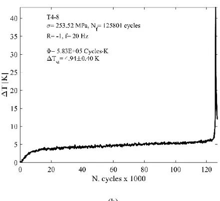
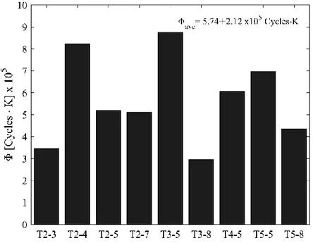
As the applied stress is higher compared to the fatigue limit of the material, the higher is the stabilization temperature, but, on the other hand, the subtended are of the temperature vs. number of cycle curve, equal to the Energy Parameter Φ, can be considered constant, given a fixed stress ratio R and test frequency. To estimate Φ, it is convenient to discard the stress levels for which it is difficult to identify the three phases (near the yielding strength of the material.

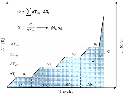
It is possible to evaluate the whole fatigue curve of the material adopting a very limited number of specimens. Given the fact that the stabilization temperature is reached in short number of cycle, it is possible to apply in a stepped way a stress level sequence, recording the stabilization temperature, till the failure of the specimen (Figure 1.7). The Energy Parameter can be estimated

(28)

13

as the integral of the temperature curve and, by the experience of the Authors, it can be evaluated, for a constant amplitude test, in a simple way as:

Φ ≈ Δ𝑇𝑠𝑡⋅ 𝑁𝑓 (1.8)

Where it is assumed that Phase I and Phase III are negligible compared to the Phase II (valid for stress levels near the fatigue limit). On the basis of equation (1.8), it is possible to evaluate the number of cycles at which the specimen would break if it were stressed only at stress level σi. The points represented by the abscissa and ordinate, respectively, equal to the number of cycles and the stress level, can be reported in a S-N diagram to obtain the whole fatigue curve of the specimen (Figure 1.8).

Figure 1.7: Stepwise fatigue test to obtain the stabilization temperature and the Energy Parameter Φ.

(29)

14

Figure 1.8: S-N curve as evaluated by mean of the stepwise fatigue test.

Several studies have been performed on different materials and applications by many researchers, validating the Thermographic Method [10,19,47–58].

The Thermographic Method, proposed by Risitano and coworkers, is a rapid test procedure able to derive, in a very short amount of time and with a limited number of specimens, the fatigue properties of the material evaluating its temperature evolution.

1.4. Energy based approach

The temperature measurement, if no precautions are taken into account, may be affected by the boundary conditions; for example, room temperature, reflecting sources and heat exchange with the grip section of the testing machine. Based on the classical continuum mechanics, some researchers [59,60], developed energy based approaches to overcome the previously mentioned problem.

The energy balance equation (first principle of thermodynamics) has been reported in terms of power per unit volume, introducing the Helmotz free energy as a thermodynamics potential [60,61]: ρc𝜕𝑇̅ 𝜕𝑡 − 𝜆∇ 2_{𝑇̅ =} 𝜕𝑊̅ 𝜕𝑡 − 𝜕𝐸̅̅̅_𝑠 𝜕𝑡 (1.9)

(30)

15

The power quantities of equation (1.9) are averaged over one cycle of fatigue loading, according to [62]. The term W represent the plastic energy, Es the stored energy, T is the material temperature, λ the thermal conductivity of the material and ρ the material density and c the specific heat.

As previously stated in section 1.2, only a part of the total energy spent in the material, introduced by fatigue loading, is stored into the material as internal energy and leading to fatigue failure. A very large amount is dissipated into the form of heat, leading to an increase of the specimen temperature.

In equation (1.9), the contribution of the thermoelastic effect has been neglected, due it reversibility that not lead to an energy dissipation. In addition, the dependence of the material from the temperature variation has been also neglected.

It is possible to define the internal energy rate as stated by Roussellier [63]:

𝜕𝑈 𝜕𝑡 = 𝜌𝑐 𝜕𝑇 𝜕𝑡 + 𝜕𝐸_𝑠 𝜕𝑡 (1.10)

If the average heat rate per cycle is defined as:

𝜕𝑄̅

𝜕𝑡 = 𝜆 ⋅ ∇

2_𝑇̅ (1.11)

It is possible to write equation (1.9) as:

𝜕𝑈̅ 𝜕𝑡 = 𝜕𝑊̅ 𝜕𝑡 + 𝜕𝑄̅ 𝜕𝑡 (1.12)

The previous equation represents an energy balance where the mechanical energy W and the dissipated heat energy Q, taken as average value over a cycle, are involved (Figure 1.9).

(31)

16

Figure 1.9: Energy balance for a material undergoing fatigue loading.

Equation (1.9), since all the quantities are averaged over a cycle, represent the average evolution of the temperature per cycle. According to this equation, the temperature can be related to the thermal energy dissipated in an elementary volume of material, but the temperature is severally affected by the experimental (thermal and mechanical) boundary conditions (specimen geometry, room temperature and test frequency). On the other hand, the energetic quantities W and Q are independent of the thermal and mechanical boundary conditions [59,64–66].

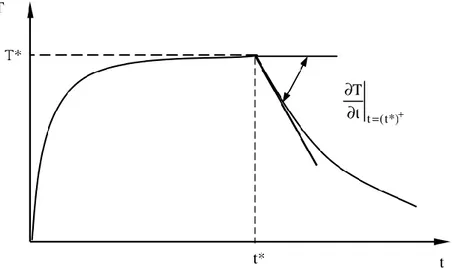
According to Meneghetti [67], during a fatigue test, when the temperature stabilizes, its thermal average derivate becomes null, hence equation (1.12), considering the relation between the internal energy rate and the stored energy (equation (1.10)), becomes:

𝜕𝐸̅̅̅𝑠 𝜕𝑡 = 𝜕𝑊̅ 𝜕𝑡 + 𝜕𝑄̅ 𝜕𝑡 (1.13)

If during a fatigue test the external work is removed suddenly (W= 0) at a time t*_{, then the} internal stored energy become zero, hence equation (1.13) can be rewritten as:

𝜕𝑄̅ 𝜕𝑡 = 𝜌𝑐

𝜕𝑇

(32)

17

Where the energy heat rate Q dissipated to the surrounding ambient is continuous in terms of time. It is possible to assess the thermal energy release in a unit of volume per cycle. It can be estimated in an easy way taking into account the test frequency f:

𝑄̅ = 𝜕𝑄̅ 𝜕𝑡 𝑓 = 𝜌𝑐𝜕𝑇_{𝜕𝑡 |} 𝑡>𝑡∗ 𝑓 (1.15)

By means of equation (1.15) it is possible to perform measurements of the specific heat loss at any point over the specimen surface (e.g. notched region [68]), during a fatigue test simply stopping the test after that the stabilization temperature has been reached (Figure 1.10).

Figure 1.10: Determination of Q by measuring the experimental thermal cooling gradient. From [67]

Compared to the Thermographic Method, where it is possible to perform temperature measurement at a coarse sample rate, even in the order of 1 image per minute for HCF regimes; the evaluation of the temperature cooling curve requires a very high frame rate to perform a good estimation of the cooling gradient.

A comparison of the experimental thermal methods on stainless steel specimen has been reported in the work of Ricotta et al. [69].

(33)

18

2. E

NERGETIC RELEASE IN STATIC TENSILE TEST

In the present chapter, the energetic release of a specimen under static tensile test condition is presented. From 1985, thanks to the development of thermocouples and infrared thermography, it has been possible to evaluate the temperature trend of specimen during monotonic tensile test. Nowadays the analysis of the energetic release in static test condition can provide useful information also on the fatigue behavior of the material.

In section 2.1 and 2.2, are presented the constitutive relation between the thermal field and the stress-strain field. Such relations are derived for isotropic and orthotropic material, considering that this two material models are the most adopted in practical application (isotropic model for metal and plastic material, orthotropic for many composite material). The fundamental relation that link the stress field to the thermal field under elastic condition, as observed by Lord Kelvin [70] in 1853, is presented. This relation describes the thermoelastic effect.

In section 2.3 are presented the early studies on the energetic release of metallic and composites specimens. Caglioti suggested to adopt the temperature analysis as a useful aid to assess some material properties difficult to evaluate only by means of the stress and strain fields. Melvin, for the first time, correlated the energetic release under static tensile test to the internal microstructure of the material. The presence of internal micro defect, hence the rise of micro plasticization phenomena, severally affect the temperature trend, showing a deviation from the linearity of the thermoelastic effect, as the applied stress increases.

In section 2.4, the Static Thermographic Method is presented. Moving to the previous studies, Risitano and Risitano defined the end of the thermoelastic effect as the limit stress of the material, where the first micro plasticization arises within the material. They linked this stress value to the conventional fatigue limit of the material. In the same section, two model to predict the temperature trend are presented. The first model requires an experimental calibration and it is able to predict with good agreement the experimental temperature trend of metallic material. The

(34)

19

second model is proposed by the author, and is suitable to be adopted with finite element simulation, as is done in further chapters of Part II of this thesis.

2.1. Stress-Strain-temperature constitutive relationship

Prior to describe the fundamental aspect of the Static Thermographic Method, it is necessary to provide an inside on the constitutive relationship between the stress-strain field and thermal field within the material. In the most general form of constitutive relations, proposed by Duhamel and Neuman [71,72], the effect of thermal and hygroscopic strains is taken into account:

{𝜎} = [𝐶]{𝜀} − [𝛽](𝑇 − 𝑇₀) − [ϕ](𝑀 − 𝑀₀) (2.1)

Where [C] represent the fourth-order elastic isothermal stiffness tensor with 21 independent components, [β] is the second-order thermal expansion tensor, T0 is the reference temperature and M0 is the reference humidity. The humidity effect in thermoelastic analysis could be neglected for sake of simplicity, hence the equation (2.1) could be formulated as [71]:

{𝜎} = [𝐶]({𝜀} − {𝛼}Δ𝑇) (2.2)

[𝛽] = [𝐶]{𝛼} (2.3)

The term {α} is the second-order coefficient of thermal expansion tensor. Under the hypothesis of homogeneous isotropic bodies, equation (2.2) can be reformulated adopting the Lamè constant [71], here reported in expanded form:

𝜎₁₁ = (2𝜇 + 𝜆)𝜀₁₁+ 𝜆𝜀₂₂+ 𝜆𝜀₃₃− 𝛾Δ𝑇 (2.4)

𝜎₂₂ = 𝜆𝜀₁₁ + (2𝜇 + 𝜆)𝜀₂₂+ 𝜆𝜀₃₃− 𝛾Δ𝑇

(35)

20 𝜎₁₂ = 2𝜇𝜀₁₂ 𝜎23 = 2𝜇𝜀23 𝜎₃₁ = 2𝜇𝜀₃₁ Or in a condensed form: 𝜎𝑖𝑗 = 2𝜇𝜀𝑖𝑗+ (𝜆𝜀𝑘𝑘− 𝛾Δ𝑇)𝛿𝑖𝑗 (2.5)

Where δij the Kronecker’s symbols (1 if i=j; 0 if i≠j). The following expressions are adopted for the Lamè constants, where α is the linear thermal expansion coefficient for isotropic material:

𝜇 = 𝐸 2(1 + 𝜈), 𝜆 = 𝜈𝐸 (1 + 𝜈)(1 − 2𝜈) (2.6) 𝐺 = 𝜇 , 𝐸 =𝜇(3𝜆 + 2𝜇) 𝜆 + 𝜇 , 𝜈 = 𝜆 2(𝜆 + 𝜇), 𝛾 = (3𝜆 + 2𝜇)𝛼 = 𝐸𝛼 1 − 2𝜈

2.1.1. First stress invariant and first strain invariant

Considering equations (2.4) or (2.5) it is possible to obtain a relation between the first stress invariant (sum of the hydrostatic pressure or sum of the principal stress) and the first strain invariant. By summing the first three terms of equation (2.4), it is possible to obtain the following expression for the first stress invariant:

Δ𝐼_1,𝜎 = (2𝜇 + 3𝜆)(𝜀₁₁+ 𝜀₂₂+ 𝜀₃₃) − 3𝛾Δ𝑇 = (2𝜇 + 3𝜆)Δ𝐼_1,𝜀− 3𝛾Δ𝑇 (2.7)

(36)

21 Δ𝐼_1,𝜀 = 1

(2𝜇 + 3𝜆)Δ𝐼1,𝜎+ 3𝛾Δ𝑇 = 𝛼

𝛾Δ𝐼1,𝜎+ 3𝛾Δ𝑇 (2.8)

Where the relation between the Lamè constant γ and α of equation (2.6) has been considered. The same expression can be formulated considering the elastic modulus and the Poisson ratio of the material:

Δ𝐼_1,𝜀 = 1 − 2𝜈

𝐸 Δ𝐼1,𝜎 + 3𝛼Δ𝑇 (2.9)

2.1.2. Plane stress condition

Under the hypothesis of a plane stress field, equations (2.5) can be written in an easier form, given the fact that σ33= σ23= σ31= 0. By substituting equation (2.6) into σ11 stress of equation (2.4) the following expression is obtained:

𝜎₁₁ = 𝐸

(1 + 𝜈)(1 − 2𝜈)[(1 − 𝜈)𝜀11+ 𝜈(𝜀22+ 𝜀33) − (1 + 𝜈)𝛼Δ𝑇]

(2.10)

From the expression of σ33 of equation (2.9), imposing the equality to 0, the expression of ε33 as a function of ε11 and ε22 could be obtained and then it can be substituted to equation (2.10).

𝜀33 = 1 + 𝜈 1 − 𝜈𝛼Δ𝑇 − 𝜈 1 − 𝜈(𝜀11+ 𝜀22) (2.11) 𝜎₁₁ = 𝐸 1 − 𝜈2(𝜀11 + 𝜈𝜀22) − 𝐸 1 − 𝜈𝛼Δ𝑇 (2.12)

Adopting the same procedure, an equivalent expression for σ33 and for the in-plane shear stress can be obtained. The stress-strain-temperature relation in the case of a plane stress field can be expressed as follows:

(37)

22 𝜎₁₁ = 𝐸 1 − 𝜈2(𝜀11 + 𝜈𝜀22) − 𝐸 1 − 𝜈𝛼Δ𝑇 (2.13) 𝜎₂₂ = 𝐸 1 − 𝜈2(𝜀22 + 𝜈𝜀11) − 𝐸 1 − 𝜈𝛼Δ𝑇 𝜎₁₂ = 𝐸 1 + 𝜈𝜀12

2.2. Thermodynamics of the elastic continuum

The general expression of the thermoelastic law in the more general case of an anisotropic material was developed by Potter and Graves [73]. They developed a formulation were the temperature variation of a solid material were bind to its deformation field under adiabatic conditions. The first principle of thermodynamics can be expressed in the following form, linking the internal energy of the system u with the work applied w and the heat provided to it q.

𝑑𝑢 = 𝛿𝑤 + 𝛿𝑞 (2.14)

The internal energy differential is expressed as an exact differential, with letter d, because it is a state variable (i.e. independent on the transformation path followed by the system), while the applied work and heat differential are expressed with inexact differential symbol δ, because they are dependent on the transformation path followed by the system to move from one state to another. The elementary work needed to deform a material volume unit, considering the stress and strain tensors is:

𝛿𝑤 = {𝜎}𝑇_{𝑑𝜀} _(2.15)

Substituting equation (2.15) into (2.14), the first principle of thermodynamics could be expressed as:

(38)

23

𝑑𝑢 = {𝜎}𝑇_{{𝑑𝜀} + 𝛿𝑞} _(2.16)

Under the hypothesis of reversible transformation, the second principle of thermodynamics states that:

𝑑𝑆 =𝛿𝑞

′

𝑇

(2.17)

Where T is the absolute temperature, S the mass entropy of the system and q’ the provided heat per mass unit. Combining equations (2.16) and (2.17), and introducing the density of the material ρ in order to refer equation (2.17) to the volume unit, equation (2.18) is obtained:

𝑑𝑢 = {𝜎}𝑇_{{𝑑𝜀} + 𝜌𝑇𝑑𝑆} _(2.18)

The Helmotz’s free energy is another state variable expressed as:

𝐻 = 𝑢 − 𝜌𝑇𝑆 (2.19)

The total differential expression of this state variable can be developed taking into account the conservation of the mass and imposing a constant density:

𝑑𝐻 = 𝑑𝑢 − 𝜌𝑇𝑑𝑆 − 𝜌𝑆𝑑𝑇 (2.20)

Substituting (2.18) into (2.20) the following expression is obtained:

𝑑𝐻 = {𝜎}𝑇_{{𝑑𝜀} − 𝜌𝑆𝑑𝑇} _(2.21)

Considering the constitutive law of the material, in this case a perfectly solid linear elastic material, the link between the stress tensor, strain tensor and temperature can be expressed as:

(39)

24

{𝜎} = [𝐶]({𝜀} − {𝛼}Δ𝑇) (2.22)

In this expression, only two within the variables {σ}, {ε} and T are independent, hence the state of the material could be identified adopting, for example {ε} and T. Given the fact that the Helmotz’s free energy is a state variable, it depends only by the strain tensor and temperature; hence it can be derived respect this two independent variables:

𝑑𝐻 = {𝜕𝐻 𝜕{𝜀}} 𝑇 𝑑{𝜀} +𝜕𝐻 𝜕𝑇𝑑𝑇 (2.23)

Comparing equations (2.21) and (2.23), the following expression for the partial derivate of the Helmotz’s free energy can be obtained:

{𝜕𝐻 𝜕{𝜀}} 𝑇 = {𝜎}𝑇 ; 𝜕𝐻 𝜕𝑇 = −𝜌𝑆 (2.24)

Entropy is also a state variable, hence it depends from the strain tensor and temperature. Its differential can be expressed as:

𝑑𝑆 = { 𝜕𝑆 𝜕{𝜀}} 𝑇 𝑑{𝜀} +𝜕𝑆 𝜕𝑇𝑑𝑇 (2.25)

Taking into account the previous equation,

𝜌𝑑𝑆 = { 𝜕 2_𝐻 𝜕{𝜀}𝜕𝑇} 𝑇 𝑑{𝜀} +𝜕 2_𝐻 𝜕𝑇2𝑑𝑇 (2.26)

The next step is to delete di entropy and Helmotz’s free energy from the previous equation; hence it is useful to derive to respect the temperature the first expression of equation (2.24).

(40)

25 { 𝜕 2_𝐻 𝜕{𝜀}𝜕𝑇} 𝑇 = 𝜕{𝜎} 𝑇 𝜕𝑇 (2.27)

This expression, together with equation (2.17), can be substitute into (2.27):

𝜌𝛿𝑞 ′ 𝑇 = − 𝜕{𝜎}𝑇 𝜕𝑇 𝑑{𝜀} − 𝜕2𝐻 𝜕𝑇2𝑑𝑇 (2.28)

It is possible to obtain a useful expression of the second derivative of the Helmotz’s free energy in equation (2.28), by substituting in the same equation the differential operator d with the partial derivative operator: 𝜌 𝑇( 𝛿𝑞′ 𝜕𝑇) 𝜀 = −𝜕{𝜎} 𝑇 𝜕𝑇 ( 𝜕{𝜀} 𝜕𝑇 ) 𝜀 −𝜕 2_𝐻 𝜕𝑇2( 𝜕𝑇 𝜕𝑇)_𝜀 (2.29)

Bearing in mind that the partial derivate is performed under the constant deformation hypothesis, the previous equation became:

𝜌 𝑇( 𝛿𝑞′ 𝜕𝑇) 𝜀 = −𝜕 2_𝐻 𝜕𝑇2 (2.30)

Introducing the heat mass capacity related to constant deformation:

𝜕2_𝐻

𝜕𝑇2 = −

𝜌𝐶_𝜀 𝑇

(2.31)

Considering the equation (2.29) and substituting the previous equation:

𝜌 𝑇( 𝛿𝑞′ 𝜕𝑇) 𝜀 = −𝜕{𝜎} 𝑇 𝜕𝑇 𝑑{𝜀} − 𝜌𝐶_𝜀 𝑇 𝑑𝑇 (2.32)

(41)

26

equation (2.22), derived respect the temperature under constant deformation:

(𝜕{𝜎} 𝜕𝑇 ) 𝜀 = (𝜕[𝐶] 𝜕𝑇 ) 𝜀 ({𝜀} − {𝛼}Δ𝑇) − [𝐶] ({𝛼} + Δ𝑇 (𝜕{𝛼} 𝜕𝑇 ) 𝜀 ) (2.33)

If the constant deformation index is omitted:

𝜕{𝜎}𝑇 𝜕𝑇 = ({𝜀} 𝑇_{− {𝛼}}T_Δ𝑇)𝜕[𝐶] 𝜕𝑇 − [𝐶] ({𝛼} 𝑇_{+ Δ𝑇}𝜕{𝛼} 𝑇 𝜕𝑇 ) (2.34)

The previous equation could be introduced in equation (2.32), hence writing:

𝜌 𝑇 𝛿𝑞′ 𝜕𝑇 = − [({𝜀} 𝑇_{− {𝛼}}T_Δ𝑇)𝜕[𝐶] 𝜕𝑇 − [𝐶] ({𝛼} 𝑇_{+ Δ𝑇}𝜕{𝛼} 𝑇 𝜕𝑇 )] 𝑑{𝜀} + 𝜌𝐶𝜀 𝑇 𝑑𝑇 (2.35)

That, under adiabatic condition, given that δq’ is null:

𝜌𝐶_𝜀 𝑇 𝑑𝑇 = [({𝜀} 𝑇_{− {𝛼}}T_Δ𝑇)𝜕[𝐶] 𝜕𝑇 − [𝐶] ({𝛼} 𝑇_{+ Δ𝑇}𝜕{𝛼}𝑇 𝜕𝑇 )] 𝑑{𝜀} (2.36)

Assuming that the reference temperature respects which the constitutive equation has been written is the average temperature of the sinusoidal stressed material, hence ΔT is the temperature excursion caused by the cyclic deformation Δ{ε}. The previous equation can be rewritten as: 𝜌𝐶_𝜀Δ𝑇 𝑇 = [({𝜀} 𝑇_{− {𝛼}}T_Δ𝑇)𝜕[𝐶] 𝜕𝑇 − [𝐶] ({𝛼} 𝑇_{+ Δ𝑇}𝜕{𝛼} 𝑇 𝜕𝑇 )] Δ{𝜀} (2.37)

This expression is at the base of the stress thermoelastic analysis. It is written in a general form, taking into account the material characteristics variation with the temperature and directions, i.e. anisotropic materials.

(42)

27

2.2.1. Isotropic material

Under the hypothesis of an isotropic material, some simplifying assumptions can be made in order to excise some terms and to obtain a simplified formulation that link directly the thermoelastic signal with the first stress invariant. For an isotropic material the stiffness matrix [C] has only two independent parameters (E and ν) and the thermal expansion vector has only one coefficient α, for normal deformation contribute; zero for the shear contribute. Another simplifying hypothesis is that is possible to neglect the variation of the elastic characteristic and of the expansion coefficient with the temperature.

{𝛼}𝑇 _{= {𝛼, 𝛼, 𝛼, 0,0,0}} _(2.38) 𝜕[𝐶] 𝜕𝑇 = 0 𝜕{𝛼}𝑇 𝜕𝑇 = 0 (2.39)

Under these assumption, equation (2.37), became:

𝜌𝐶_𝜀Δ𝑇

𝑇 = −{𝛼}

T_{[𝐶]Δ{𝜀}} (2.40)

Developing the second member of the previous equation:

𝜌𝐶_𝜀Δ𝑇 𝑇 = −𝛼 𝐸 (1 + 𝜈)(1 − 2𝜈){(1 + 𝜈), (1 + 𝜈), (1 + 𝜈)}𝑇Δ{𝜀} (2.41) 𝜌𝐶_𝜀Δ𝑇 𝑇 = −𝛼 𝐸 (1 − 2𝜈)(Δ𝜀𝑥𝑥 + Δ𝜀𝑦𝑦+ Δ𝜀𝑧𝑧) = −𝛼 𝐸 (1 − 2𝜈)Δ𝐼1,𝜀 (2.42)

Instead of the first deformation invariant, it is convenient to rewrite the equation (2.42) adopting the first stress invariant (equation (2.9)):

𝜌𝐶_𝜀Δ𝑇

𝑇 = −αΔI1,σ− 3𝛼

2 𝐸

1 − 2𝜈Δ𝑇

(43)

28 𝜌 (𝐶𝜀 + 3𝛼2_𝑇 𝜌 𝐸 1 − 2𝜈 ) Δ𝑇 𝑇 = −αΔI1,σ (2.44)

This equation is formally similar to the previous one and more useful from a practical point of view, given that a link between the specific heat at constant deformation and constant stress exist. It is well known that in solid materials, as well as in liquid ones, it is difficult to estimate the specific heat at constant deformation due to the high stress field that rise when the deformations are locked [74]. Despite this, a relation between the two specific heat exist, evaluated on the basis of the heat amount provided to the solid and the temperature variation at zero stress. Under these hypotheses it is possible to write [75]:

𝛿𝑞 = 𝜌𝐶_𝜎𝑑𝑇 𝛿𝑞′ _{= 𝐶}

𝜎𝑑𝑇 (2.45)

Inserting equation (2.45) in equation (2.35), taking into account all the simplifying hypotheses adopted here, the following equation can be write:

𝜌𝐶_𝜎d𝑇 𝑇 = 𝛼 𝐸 (1 − 2𝜈)Δ𝐼1,𝜀+ 𝜌𝐶_𝜀 𝑇 𝑑𝑇 (2.46)

Under the hypothesis of constant stress, it is possible to insert the first strain invariant. The following expression that link the specific heat at constant deformation with constant stress:

𝐶_𝜎 = 3𝛼 2_𝑇 𝜌 ⋅ 𝐸 1 − 2𝜈+ 𝐶𝜀 (2.47)

This relation allow to rewrite equation (2.44) as:

𝜌𝐶_𝜎Δ𝑇

(44)

29

The previous equation states that the local temperature variation is directly proportional to the first stress invariant variation of the local stress state, i.e. the variation of the hydrostatic stress component or the sum of the principal stresses. For an elastic homogeneous isotropic solid, neglecting the variation of the mechanical and thermal material properties with the temperature, it is possible to write:

Δ𝑇 = − 𝛼

𝜌𝐶_𝜎⋅ 𝑇Δ𝐼1,𝜎 = −𝐾𝑚𝑇 ⋅ Δ𝐼1,𝜎 (2.49)

The Km constant in equation (2.49) is the thermoelastic constant of the material. Some materials present negative values of the thermoelastic constant (rubber, carbon fiber, some plastic material), but in general it is positive. The typical value for this constant for steel alloys is about 3.3x10-12_Pa-1_{, while for aluminum alloys 9.5x10}-12_Pa-1_{. This constant can be assumed constant} only if the variation with temperature of the thermal expansion coefficient, the density and the specific heat can be neglected.

The thermoelastic effect is due to the interconnection between the mechanical work made on the material in the elastic field and the variation of its thermodynamics characteristics, i.e. stress-strain vs. entropy and temperature. Under an isentropic (reversible) process, the variation of the internal energy of the deformed body is due only to the mechanical work done, as stated by the first and second thermodynamics principles. For an elastic homogeneous isotropic material under uniaxial stress, equation (2.49) simplify in:

(∂T

∂σ₁)_𝑆 = −𝐾𝑚⋅ 𝑇 (2.50)

According to this equation, a traction stress in elastic regime lead to a temperature decrement, while a compression increases it. As a general rule, a crystalline material tends to cool itself when undergoes to traction condition; however, if the load velocity is extremely slow, the material absorb heat from the surrounding environment and its temperature remain constant, i.e. the process is isotherm.

(45)

30

2.2.2. Orthotropic material

For an anisotropic material with orthotropic properties, the thermal expansion coefficient vector and the stiffness matrix of the material assume the form of equation (2.51).

{ 𝜎_𝑖𝑖 𝜎_𝑗𝑗 𝜎𝑘𝑘 𝜎_𝑖𝑗 𝜎𝑖𝑘 𝜎𝑗𝑘} = [ 𝐶_{𝑖𝑖𝑖𝑖} 𝐶_{𝑖𝑖𝑗𝑗} 𝐶_{𝑖𝑖𝑘𝑘} 0 0 0 𝐶_{𝑖𝑖𝑗𝑗} 𝐶_{𝑗𝑗𝑗𝑗} 𝐶_{𝑖𝑖𝑘𝑘} 0 0 0 𝐶_{𝑘𝑘𝑖𝑖} 𝐶_{𝑘𝑘𝑗𝑗} 𝐶_{𝑘𝑘𝑘𝑘} 0 0 0 0 0 0 𝐶_{𝑖𝑗𝑖𝑗} 0 0 0 0 0 0 𝐶_{𝑖𝑘𝑖𝑘} 0 0 0 0 0 0 𝐶_{𝑗𝑘𝑗𝑘}] ⋅ ({ 𝜀_𝑖𝑖 𝜀_𝑗𝑗 𝜀𝑘𝑘 𝜀_𝑖𝑗 𝜀𝑖𝑘 𝜀_𝑗𝑘} − { 𝛼_𝑖𝑖 𝛼_𝑗𝑗 𝛼𝑘𝑘 𝛼_𝑖𝑗 𝛼𝑖𝑘 𝛼_𝑗𝑘} Δ𝑇 ) (2.51)

In order to define the stiffness matrix, nine independent parameters are required: the three normal elastic modulus, the three tangential elastic modulus and the three Poisson coefficient. If the reference system is not the same of the orthotropic axes, all the terms of the stiffness matrix and of the thermal expansion coefficient are different from zero.

For a thin lamina of material, the stress state can be assumed as planar, where three of the six independent are equal to zero (e.g. σii, σjj, σij). As regards the deformations, εik and εjk are null, while εkk is equal to:

𝜀_𝑘𝑘 = −𝐶𝑘𝑘𝑖𝑖𝜀𝑖𝑖+ 𝐶𝑘𝑘𝑗𝑗𝜀𝑗𝑗

𝐶_{𝑘𝑘𝑘𝑘} (2.52)

In an arbitrary reference system, the thermoelastic equation (2.37) for an anisotropic material, hence also for orthotropic material, under plane stress state is:

𝜌𝐶_𝜎Δ𝑇

𝑇 = −(αxxΔσxx+ 𝛼𝑦𝑦Δ𝜎𝑦𝑦+ 𝛼𝑥𝑦Δ𝜎𝑥𝑦) (2.53)

And, if the principal stress reference system is taken into account, which directions in general do not coincide with the principal directions of the deformations and material orthotropic principal directions, the thermoelastic equation (2.48) simplifies in:

(46)

31 𝜌𝐶_𝜎Δ𝑇

𝑇 = −(α11Δσ1+ 𝛼22Δ𝜎2) (2.54)

Where in the principal reference system the following expression are valid:

{𝜎} = { 𝜎₁ 𝜎2 0 } {𝛼} = { 𝛼₁₁ 𝛼₂₂ 𝛼₁₂} (2.55)

Equation (2.54) does not allow an easy assessment of the temperature value due to the fact that the principal stress direction varies locally and are unknown a priori; in addition, it is not possible to assign the thermal expansion coefficient values in these directions. On the other hand, if the reference orthotropic reference system is taken into account, the stress and thermal expansion coefficient became: {𝜎} = { 𝜎_𝑖𝑖 𝜎_𝑗𝑗 𝜎_𝑖𝑗} {𝛼} = { 𝛼𝑖𝑖 𝛼𝑗𝑗 0 } (2.56)

That are known, given that the thermal expansion coefficient are defined along the orthotropic directions. The thermoelastic equation (2.48) became:

Δ𝑇 = − 𝑇

𝜌𝐶_𝜎(αiiΔσii+ 𝛼𝑗𝑗Δ𝜎𝑗𝑗) (2.57)

Considering the temperature variation, it is possible to write in analogy to the isotropic solid equation (2.57) as:

Δ𝑇 = −𝐾_𝑚𝑇(Δσ_ii+ 𝛼_𝑚Δ𝜎_𝑗𝑗) 𝐾_𝑚 = − 𝛼𝑖𝑖

𝜌𝐶_𝜎 𝛼𝑚 = 𝛼_𝑗𝑗

𝛼_𝑖𝑖 (2.58)

Compared to the coefficient α11 and α22 in equation (2.54), the coefficient ii and jj or the Km constant and αm ratio, can be univocally determined knowing the principal directions respect to which estimate the thermal expansion coefficient.

(47)

32

2.3. Thermal behavior under static tensile test

2.3.1. Early study of the change in the temperature trend during tensile

test

In a work of 1982, Caglioti [76] studied the behavior of a material that undergoes to elastic deformation towards the “thermoelastic instability”. According to Caglioti, any mechanical transformation can be considered as an irreversible thermodynamics transformation, hence all the state variables (e.g. strain, stress and temperature) and the coupling between them must be taken into account for a clear understanding of the mechanical transformation. The consideration of the thermal behavior during mechanical tests, in particular during fatigue tests, has been taken into account recently. Assuming that entropy change measures the quality of a system transformation, when a deformation is applied to a material, it promotes two different entropy changes: a thermal entropy change and a configurational entropy change. They are of the same importance and must compensate each other during an ideally adiabatic and isentropic transformation. For example, the reason for thermoelastic cooling of metallic specimen under adiabatic tension [70]. As the applied deformation increases, the adiabatic cooling of the specimen proceeds up to a state where the deformation field promotes a positive change in the temperature field.

Caglioti proposed to adopt the whole thermoelastic region, thanks to the coupling between the thermal and mechanical transformation, as a very fine probe of the state of the material. The thermoelastic behavior can be adopted for an accurate determination of several thermal and mechanical properties of the materials itself and to predict eventually change in its mechanical behavior.

One of the main reason why the thermoelastic behavior has been neglected is due to the small temperature variation during an adiabatic elastic transformation. For example, the order of magnitude of the temperature decrement for a metal under adiabatic conditions is of the order of 0.2K, a value that in practical application has been always neglected due to the difficult to assess it. Nowadays, thanks to the development of infrared sensors, it is possible to apply the infrared thermography in an easy way on a large set of materials, even under working conditions.

Caglioti observed that when the metallic material is elastically strained, the temperature tend change in a remarkable way as the yielding stress is approaching Figure 2.1. This temperature behavior might help to identify the thermoelastic limit between the elastic and the incipient

(48)

33

plastic regime. In the work of Caglioti, the temperature versus stress diagram (ΔT-σ) for a steel sample during a monoaxial tensile test in order to determine the yielding stress of the material.

Figure 2.1: Temperature dependence on the stress reacting to the deformation imposed to a steel sample [76].

The yielding stress has been defined as the corresponding stress for which the temperature tangent is horizontal and then the temperature trend experience an increment.

2.3.2. Correlation between the energetic release and the material

microstructure

Melvin et al. studied in detail the heat generated during mono axial tensile test of several types of steel [77] and composite materials [78]. Melvin developed a model taking into account microscopic considerations on the macroscopic thermal behavior of the material. The microscopic approach involves the analysis of the atomic source of plastic strain, i.e. dislocations. On the other hand, the macroscopic approach models the material as a continuum, considering only its average properties.

Focusing on the microscopic scale, when a tensile stress is applied on a crystalline structure, such as metals, a corresponding elastic dilation is observable. The applied external work, at atomic level, is adopted to raise the interatomic potential of the vibrating body in thermal equilibrium and hence increase the mean interatomic separation. In order to oppose to the