Contributions
Fabrizio Coricelli, Aikaterini E. Karadimitropoulou*
and Miguel A. Leon-Ledesma
Reallocation effects of recessions and
financial crises: an industry-level analysis
DOI 10.1515/bejm-2015-0082Previously published online March 8, 2016
Abstract: We characterize the behavior of disaggregate manufacturing sectors for a large set of developed and emerging markets around recession dates. We uncover some relevant stylized facts. The dispersion in value added (VA) growth rates in devel-oped economies is counter-cyclical, whereas for emerging countries it is pro-cycli-cal. Recoveries are more productivity-driven in developed countries as opposed to employment-driven for emerging markets. Around recession episodes sectoral-level misallocation of resources does not significantly change in developed economies, whereas it increases in emerging economies during financial crises. Therefore, there is no evidence that recessions improve the allocation of resources across industries. Keywords: permanent productivity effects; recessions; sectoral restructuring. JEL: E32; O14; O47.
1 Introduction
There is increasing interest in analyzing the behavior of the economy during recession episodes, and how these temporary events can have long-lasting effects by shaping the productive structure of the economy. This interest has gained importance with the 2008/2009 financial crisis and global recession. Most of the existing literature focuses on recessions at the aggregate level.1 We
*Corresponding author: Aikaterini E. Karadimitropoulou, Department of Economics, University of East Anglia, Norwich, Norfolk NR4 7TJ, UK, e-mail: [email protected]
Fabrizio Coricelli: Department of Economics, Paris School of Economics, 75013, Paris, France and CEPR
Miguel A. Leon-Ledesma: School of Economics and Macroeconomics, Growth and History Centre (MaGHiC), University of Kent, CT27NP, Canterbury, UK
1 See Cerra and Saxena 2008, Reinhart and Rogoff 2009b. One recent exception is Claessens, Tong, and Wei (2012) who examined, firstly, how the performance of firms was affected by the
take a step towards understanding the behavior of economies around recession periods at a more disaggregate level by looking at industrial data for a set of 37 developed (hereafter, DV) and emerging (hereafter, EM) economies. Our study addresses several questions. First, are recessions more industry-specific events or do they affect most industrial sectors? Second, depending on the productiv-ity level and on the level of external financial dependence (EFD), how do key macroeconomic variables and sectoral shares evolve during a recession in DV as compared to EM markets? Third, is this behavior different in the case of financial recessions? Fourth, do recession episodes lead to concentration/specialization of value added (VA) and employment shares? Fifth, are country-level productivity changes around recessions driven by changes in labor productivity growth within industries or by changes in the allocation of labor across industries? Finally, do recessions change the level of resource misallocation across industrial sectors?
To address these questions, we take a purely descriptive yet information-rich approach. We analyze a total of 120 recessions, among which 29 are identified as financial crises, for 28 industries for a set of 37 DV and EM economies. For each country, recessions are identified as observations where GDP displays negative growth. This enables us to detect which industries are facing a drop in VA growth in recession years and to analyze whether recession episodes tend to be more con-centrated on a few industries or they are sector-wide events. We then focus on the evolution of VA, employment, productivity, industrial concentration and sec-toral shares, distinguishing between EM and DV economies and between sectors depending on either their productivity level or their level of EFD. We also make use of industry concentration indexes to examine whether recessions are associated with any significant changes in the degree of concentration of VA and employment. We can interpret concentration as “specialization,” that is, whether a significant proportion of output (inputs) in the economy is being produced (used) by a few industries. Finally, we make use of a decomposition analysis to identify whether changes in productivity growth are linked to differential growth of labor productiv-ity or to the reallocation of labor between industries. Although it is not possible to extract meaningful causal or structural interpretations from our results, they provide a set of stylized facts that are useful for both policy and model building.
Our research can be placed within several strands of related literature. As Lien (2006) argues, however, most of the existing evidence is a “byproduct” arising from research focusing on aspects other than the disaggregate behavior in recessions. There is, nonetheless, a wide body of theoretical literature on the
2007–2009 crises and secondly, the channels (i.e. a business cycle channel, a trade channel and a financial channel) through which the crisis is propagated. Their results show that the decline in profits and sales of firms increases the more sensitive the firm is to a demand or trade shock. Finally, trade linkages are far more important in explaining the spillover of crises.
reallocation effects of recessions (i.e. Hall 1991; Caballero and Hammour 1994)2
and a body of empirical literature analyzing the long-lasting effects of reces-sions and financial crises (i.e. Cerra and Saxena 2008; Reinhart and Rogoff 2008, 2009a).3 The latter focuses on aggregate time-series evidence, and aims at
unveil-ing whether recovery after a recession is complete or partial, and whether finan-cial crises are associated to deeper and more persistent recessions. This evidence, although very relevant, cannot dissect what lies behind these potential perma-nent effects: reallocation of factors of production, within sector productivity effects, permanent changes in the level of sectoral investment and employment, etc. Our study is a first step to fill this gap. Our descriptive analysis enables us to characterize business cycles across industries in recession years. This examina-tion is important for understanding the sources of business cycles. Research on business cycle transmission at the sectoral level has attracted increasing interest since Long and Plosser (1987). They used factor analysis to estimate the impor-tance of disaggregate shocks in the US. Their results show that, although dis-aggregate shocks are important, dis-aggregate shocks remain the most important source of industrial output fluctuations. Similar results were shown by Norrbin and Schlagenhauf (1988, 1990) and Pesaran, Pierse, and Lee (1993). Recently, Chang and Hwang (2015) analyze business cycle co-movement for a set of 74 industrial sectors in the US economy. They show that there is a high degree of comovement during phases of the business cycle and that troughs tend to be more concentrated than peaks. Karadimitropoulou and León-Ledesma (2013) highlight the importance of understanding international output fluctuations from a multi-sector perspective and show that sectors play a non-negligible role in the transmission of international output fluctuations. Imbs (2004) argues that, given that individual industries are subject to common shocks, two countries with similar production structure will be subject to greater co-movement. Clearly, understanding how economies respond to recessions at a disaggregate level is crucial for both policies and model- building (Cerra and Saxena 2008). Although we also report concordance indicators for traditional business cycles, our focus is on recession episodes. The motivation for this focus is not only that recessions tend to lead to long-lasting effects, but also because business cycles character-istics tend to differ across DV and EM economies. Aguiar and Gopinath (2007) show that in contrast to DV countries, EM markets are characterized by recurrent
2 See also, amongst others, Stadler (1990) and the R&D models of Aghion et al. (2005) and Barlevy (2007) and the empirical evidence at the micro level in Davis, Haltiwanger, and Schuh (1996). 3 Further evidence can be found in Arbache and Page (2010), Ceccheti, Kohler, and Upper (2009), Christopoulos and León-Ledesma (2014), Claessens, Kose, and Terrones (2008), Eichengreen and Rose (1998), and Kaminsky and Reinhart (1999) amongst many others.
shocks to growth rates rather than output levels. Therefore, in an international comparison, the NBER approach focusing on recessions and recoveries (peak-trough-recovery phase) seems more appropriate than the standard business cycle approach, which focuses on deviations of output from trend. Finally, the comparison between EM and DV countries is particularly relevant as goods and factor market institutions significantly differ across advanced and EM economies, especially with respect to the functioning of labor and financial markets. This is crucial both for the transmission of shocks and the ability to support an efficient reallocation of resources across sectors.
Our main results are as follows. While EM markets display more dispersion in VA growth rates and hence more industry-specific recessions, this dispersion behaves counter-cyclically for DV countries and pro-cyclically for EM markets. On the other hand, by analyzing the concordance of industries during business cycle phases we conclude that expansions tend to be more coordinated across industries for EM markets. Moreover, whether industries are grouped in terms of their productivity level or their level of EFD, the amplitude of the cycle for VA and productivity growth is larger for EM markets. The opposite is generally true for employment growth. Regarding VA and employment shares, in DV countries there seems to be a mild redistribution from the lowest productivity group to the other groups. This only holds for employment shares in EM. Overall, around recession episodes sectoral-level misallocation of resources does not significantly change in developed economies, whereas it increases in emerging economies during financial crises. Therefore, there is no evidence that recessions improve the allocation of resources across industries. Furthermore, when looking at the level of EFD, industries with high dependence on external finance generally face higher contractions in VA growth during the recession year(s) and, especially during financial crises. Also, this same group of industries generally displays faster output growth after a recession than industries with low financial depend-ence, consistent with Kroszner, Laeven, and Klingebiel (2007).
During financial recessions, VA growth tends to follow a W-shape pattern (Kannan 2009). That is, although 1 year after the recession growth has recovered to pre-recession levels, most of the industries face a larger contraction 2 years fol-lowing the episode. We also find that changes in industrial concentration around recessions are small for both groups of countries. Finally, country-level produc-tivity changes are mainly driven by changes in labor producproduc-tivity growth within industries rather than changes in the industrial structure.
The rest of the paper is organized as follows. Section 2 discusses the data. Section 3 describes recession episodes at the aggregate and sectoral level. Section 4 discusses the methodology used for the descriptive analysis. Section 5 presents the results and, finally, Section 6 concludes.
4 It may have been possible to overcome this problem by making use of the EU KLEMS data-base, which provides measures of output, value added, employment by skills, capital, energy and material inputs, and multi-factor productivity at the sectoral level for the European Union, the US, South Korea and Japan. However, the main disadvantage of this database is that it limits the sample coverage only to OECD countries.
5 Imbs and Wacziarg (2003) report that measures such as industrial concentration and speciali-zation for UNIDO tend to display less variation than databases containing other sectors such as agriculture, mining and services. However, this pattern is exclusive to rich countries.
2 Data description
We make use of the UNIDO Industrial statistics database (INDSTAT). The INDSTAT, in accordance with Revision 2 of the International Standard Industrial Classifica-tion of All Economic Activities (ISIC), presents the dataset arranged at the 3-digit level of the ISIC code, which provides 28 industrial branches of the manufactur-ing sector (plus the total manufacturmanufactur-ing aggregate). Appendix A lists the manu-facturing industries with their associated ISIC codes. The fact that the dataset only covers the manufacturing sector is also its main disadvantage.4 Especially in
DV economies, the border between manufacturing and service is increasingly ill defined, as manufacturing firms outsource several activities and they make use of temporary agency works (Estevao and Lach 1999 for the US). Employing workers from temporary agency services induces an underestimation of employment in manufacturing and, as a result, it induces an overestimation of labor productiv-ity growth in manufacturing. Nevertheless, in order to carry out a comparison between DV and EM economies over a relatively long time interval the UNIDO dataset is more suitable for this study.5 It is also likely that input and output data
in services sectors is also subject to greater measurement error. Finally, the man-ufacturing sectors typically undergo sharper fluctuations in recession-recovery episodes, while services tend to behave more smoothly. Therefore, manufactur-ing remains central for studymanufactur-ing adjustments durmanufactur-ing recession episodes.
A key element of our analysis is the possible heterogeneity of behavior in emerging (EM) and advanced economies (DV). To classify countries in the two groups we used the FTSE Global Equity Index Series Country Classification in 2008. Thus, our classification is based on an-end period reference date. This classification combines gross national income (GNI) per capita with indicators of integration of countries in international financial markets. Admittedly, the degree of international financial integration becomes much more relevant after the 1990s. As the classification is not available for the 1970s and 1980s, we cannot directly verify whether there is migration over time from one category to the other. Nevertheless, if we had used other common classifications, such as OECD vs non-OECD countries, we would have obtained a stable grouping with the exception of
Israel, which joined the OECD in 2010, and Singapore, which is not a member of the OECD.
We also collected data for annual GDP growth from the World Bank WDI data-base in order to identify the recession years. The business cycle dating literature normally uses quarterly indicators as in the NBER definition of recessions, but quarterly data are not available for the majority of countries selected. Recessions are then identified as observations where GDP displays negative growth. We con-sider not only a definition of “deep recession” when the GDP percentage drop is larger than the mean drop of output in all the recessions faced by the other countries in the sample, but also a definition of deep recessions where the mean output drop for comparison is split depending on the country group (DV and EM). This is because GDP growth tends to be more volatile in EM economies. By com-paring them to all countries, we would be considering too many deep recessions, especially because DV countries are over-represented due to data availability.6
We also used a cycle concordance analysis following Harding and Pagan (2002) where, instead of focusing only on recessions, we analyze the different phases of the business cycle (i.e. peaks and troughs).
The UNIDO dataset spans the 1963–2003 period. However, data availability for the 1963–1969 period and for 2003 is very limited, so we effectively limited the study to the 1970–2002 period. The sample selection of countries and periods from the UNIDO dataset was based on data availability. We used three criteria for the inclusion of countries. Firstly, we require at least 18 years of observations (half of the available sample) to ensure data was not available only for certain periods, especially when the country reaches a certain level of development. Secondly, we require data availability for at least 13 industrial branches of the manufactur-ing sector (roughly half the number of branches). Finally, every country in the sample must have experienced at least one recession according to the definition above. Based on those criteria, a total of 37 countries were selected for the analy-sis, including 22 DV and 15 EM economies. Because of discontinuities and gaps in the data, missing values of up to 3 years in the observations were recovered by data interpolation.7 The number of sectors remains constant in each country over
time; however, it does vary across countries.
VA data are given in nominal terms and UNIDO does not provide sectoral VA deflators. It does, however, contain industrial production data, which are in “volume” index number, as well as nominal output data for all countries. Using
6 Deep recessions are only used for the analysis of the incidence, duration and amplitude of recessions at the aggregate level.
these data we then obtained production deflators for each branch and country.8
West Germany was the only country for which the “volume” index was not avail-able and, therefore, we made use of the EU KLEMS dataset that provides the VA Manufacturing deflator at a disaggregated level from 1970 to 1991. VA was then deflated to obtain real VA (RVA) in the standard way: RVAijt = VAijt/PYijt, where PY is the output deflator, j is a country index, i is an industry branch index, and t is the time index. This also enables us to construct the real labor productivity level as the level of RVA in local currency per worker (L): LPijt = RVAijt/Lijt. Data on capital stock were not available and, because investment data are very sparse and available only for a few countries, we cannot build measures of capital stock using standard inventory methods. Hence, although arguably a less satisfactory measure of productivity than TFP, labor productivity ensures less measurement error. Also, LP will reflect productivity effects coming from both supply and demand shocks.
3 Recessions: characteristics, co-movement,
and concordance
We fist analyze the characteristics of aggregate recessions and their incidence by industry to unveil the degree of coordination between industries during recession events. We then describe the degree of business cycle concordance looking at both troughs and peaks of the cycle.
3.1 Incidence, duration and amplitude of recessions
From 1970 to 2002, we observe 120 recessions for the 37 country sample as reported in Table 1. The Table reports the sample period for each country (column 2), the cumulative sum of the drop in GDP (column 3) and the mean GDP drop (column 4) during all recessions faced by each country, and column 5, 6, and 7 display the
8 Our choice of price deflator is induced by data availability. Using producer prices rather than VA deflators may introduce bias in our measures of real VA. We derive producer price index (PPI) by deflating nominal output by output in volumes. It can be shown (IMF 2004) that the PPI is either the lower bound (when the price index is computed at initial period technology and input structure) or the upper bound (when the price index is computed at end-period technology and input structure) of the VA deflator. In our case, PPI is the lower bound and thus it reduces the variability of sectoral prices and thus it may overstate the variability of real sectoral value added.
Table 1: List of countries and descriptive analysis of recessions.
Country Sample
period Sum drop of output Mean drop of output Nb. of REC duration Aver. of REC Nb. of deep recessions Australia 1970–2001 –3.012 –1.506 2 1.000 0 Austria 1970–2002 –0.669 –0.167 4 1.000 0 Belgium 1970–2001 –2.568 –0.856 3 1.000 0 Canada 1970–2002 –4.953 –2.477 2 1.000 1 Chile 1970–1998 –31.233 –6.247 5 1.667 4 Colombia 1970–1999 –4.204 –4.204 1 1.000 1 Denmark 1970–1991 –3.432 –0.686 5 1.667 0 Ecuador 1970–2002 –11.546 –2.887 4 1.500 1 Finland 1970–2002 –10.899 –3.633 3 3.000 2 France 1970–2002 –1.886 –0.943 2 1.000 0 Germany 1970–1991 –1.834 –0.917 2 1.000 0 Greece 1970–1998 –14.062 –2.344 6 1.500 1 Honk Kong 1973–2002 –6.026 –6.026 1 1.000 1 Hungary 1970–2002 –19.347 –3.225 6 2.000 3 India 1970–2002 –5.787 –2.894 2 1.000 1 Indonesia 1970–2002 –13.127 –13.127 1 1.000 1 Iran 1970–2002 –54.708 –4.973 11 2.500 6 Ireland 1970–2001 –0.672 –0.336 2 1.000 0 Israel 1970–2002 –1.574 –0.525 3 1.000 0 Italy 1970–2002 –2.979 –1.490 2 1.000 0 Japan 1970–2002 –3.416 –1.139 3 1.500 0 Jordan 1979–2002 –15.304 –7.652 2 2.000 1 Korea 1970–2001 –8.342 –4.171 2 1.000 1 Malaysia 1970–2002 –8.481 –4.241 2 1.000 1 Malta 1975–2000 –0.612 –0.612 1 1.000 0 Netherlands 1970–1993 –1.797 –0.899 2 2.000 0 New Zealand 1970–1987 –7.775 –1.555 5 2.000 1 Norway 1970–2001 –0.173 –0.173 1 1.000 0 Panama 1970–2000 –19.680 –6.560 3 1.500 2 Portugal 1970–2002 –8.443 –2.111 4 1.333 1 Singapore 1970–2002 –5.219 –1.740 3 1.000 0 Spain 1970–2002 –1.165 –0.583 2 1.000 0 Sweden 1970–2000 –6.046 –1.209 5 1.667 0 Turkey 1970–1997 –7.739 –2.580 3 1.500 1 UK 1970–2002 –6.910 –1.382 5 1.667 0 US 1970–2002 –3.058 –0.612 5 1.250 0 Zimbabwe 1970–1995 –22.422 –4.484 5 1.250 2 ALL –8.590 –2.734 120 1.365 32 Developed –4.207 –1.240 71 1.345 6 (All)/29 (DV) Emerging –15.237 –4.925 49 1.394 26 (All)/20 (EM) DV stands for developed countries and EM stands for emerging countries.
number of recessions, their average duration, and the number of deep recessions, respectively. Seventy-one of those recessions took place within the DV group of countries and the remaining 49 were faced by the EM markets, implying a similar number of recessions per country for both groups. However, sample periods are generally shorter for EM markets, which implies a slightly higher incidence of recessions for that group. Iran underwent the largest number of recessions, 11, between 1970 and 2002 and this clearly places it first in the sum drop of output list. Indonesia experienced the largest average fall in GDP during recessions, but it only experienced one recession in 1997. Other countries like the UK and the US faced five recessions each during the time period considered, with the impact on GDP growth being larger for the UK than for the US. Overall, we can see that the severity of recessions in EM markets exceeds that of DV countries, which is a common feature analyzed in, for instance, Aguiar and Gopinath (2007). This happens not because of a higher incidence of recessions, but because, primar-ily, recessions in the EM world are deeper. We can also see this by looking into the incidence of deep recessions. 32 out of the 120 recessions were classed as “deep” when considering all countries; six of them took place in DV countries and the remaining 26 in the EM markets. In other words, those 32 episodes pro-duced a higher drop in output than the mean drop of output faced by all countries (2.73%). When using DV and EM country averages as reference groups, we see that for DV countries 29 out of 71 recessions were considered deep, whereas 20 out of 49 recessions are deep for EM economies.
The average duration of recessions is very close for both groups of countries, only slightly shorter for the DV group. On average recessions last about 1 year and 4 months. However, it is likely that this figure is inflated because we only have annual data, setting a floor of 1 year to the minimum recession duration. Finland is the country facing the largest average duration due to the deep and long-lasting depression during the early 1990s. On average, also, recessions tend to happen every 9 years, although this number is slightly shorter for EM countries.
3.2 Industry-specific versus sector-wide recessions
A relevant feature to analyze in the data is whether recession episodes tend to be more concentrated on a few sectors or they are sector-wide events. Note that, given that we identify recessions using GDP and our UNIDO data only contains manufacturing, this may tend to underestimate the incidence of recessions with a sector-specific bias. Nevertheless, comparisons between countries are still pos-sible. Using our definition of recessions, we identify which industries are facing a drop in VA growth in recession years. This enables us to show the average
percentage of industries in recession during the episode. That is, whether reces-sions are coordinated phenomena across industries.9
Another important metric is the standard deviation of the growth rate of VA across industries within a country, which measures the dispersion of VA growth across industries during recession episodes, hence the degree of heterogeneity of performance across industries.
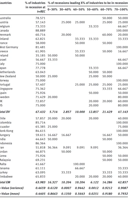
Table 2 shows the average percentage of industries facing negative VA growth during recession years (t = REC) for each country and group. It also shows the per-centage of recessions for each country where different perper-centages of industry branches showed negative VA growth. This enables us to identify whether coun-tries face predominantly industry-specific or industry-wide recessions. We can see that the average percentage of contracting industries at the time of recession episodes is slightly higher for DV than EM countries, 67.43% and 63.98% respec-tively. This difference however is found to be statistically insignificant. More pre-cisely, from the DV countries considered in this study, Canada and West Germany display the highest percentage of contracting industries at the time of the episode (85.89% and 81.48%, respectively), whereas Ireland displays the lowest percent-age out of all the countries (35.19%). From the EM countries group, we can see that in Colombia, Honk Kong, and Indonesia, 88.71%, 84.62% and 86.36% of industries, respectively, are contracting at t = REC. Malta, India and Jordan repre-sent the other extreme in this group.
Perhaps more informative is the second part of the table from which we can see that, in DV countries, 47.14% of the recessions were associated with VA con-traction for 70% or more industries, 21.43% with between 60 and 70%, 12.86% with between 50 and 60% of the industries and, finally, only 18.571% with less than 50% contracting industries. In contrast, the numbers for EM markets are consistently lower for high percentages of industries. In fact, almost 37% of reces-sions were accompanied by less than 50% of industrial branches contracting. Importantly, there is some evidence that the ratio of the variances between DV and EM countries is different to one for 2 out of the 6 grouping classifications, namely, for those groups where 30–40% and 50–60% of industries are in reces-sion at the same time that the aggregate economy is in recesreces-sion. For the second group the differences in mean between DV and EM countries were found to be strongly significant while for the first one this conclusion only applies if we use a very lax criterion such as a 15% significance level. Therefore, there seems to be some evidence, albeit limited, that recessions tend to be more coordinated across manufacturing industries in DV countries.
Table 2: Industry-specific and industry-wide recessions. Countries % of industries
in recession at
t = REC
% of recessions leading X% of industries to be in recession 0–30% 30–40% 40–50% 50–60% 60–70% 70–100% Australia 78.571 50.000 50.000 Austria 57.143 25.000 25.000 25.000 25.000 Belgium 73.333 33.333 66.667 Canada 88.889 100.000 Denmark 60.714 20.000 60.000 20.000 Finland 62.821 33.333 33.333 33.333 France 58.000 50.000 50.000 West Germany 81.481 100.000 Greece 61.905 33.333 50.000 16.667 Ireland 35.185 50.000 50.000 Israel 56.667 33.333 66.667 Italy 75.000 100.000 Japan 77.778 33.333 66.667 Netherlands 63.043 50.000 50.000 New Zealand 50.000 25.000 25.000 50.000 Norway 75.000 100.000 Portugal 57.407 25.000 25.000 25.000 25.000 Singapore 75.362 33.333 66.667 Spain 75.926 50.000 50.000 Sweden 71.429 20.000 80.000 UK 72.857 20.000 20.000 60.000 US 75.000 20.000 80.000 Total DV 67.432 5.714 2.857 10.000 12.857 21.429 47.143 Chile 57.857 20.000 20.000 20.000 40.000 Colombia 85.714 100.000 Ecuador 65.385 25.000 75.000 Honk Kong 84.615 100.000 Hungary 59.615 16.667 16.667 16.667 50.000 India 44.643 50.000 50.000 Indonesia 86.364 100.000 Iran 51.818 36.364 9.091 9.091 9.091 36.364 Jordan 46.875 50.000 50.000 Korea 75.926 50.000 50.000 Malaysia 69.231 50.000 50.000 Malta 41.667 100.000 Panama 61.111 66.667 33.333 Turkey 63.095 33.333 33.333 33.333 Zimbabwe 65.833 20.000 20.000 20.000 40.000 Total EM 63.983 16.327 10.204 10.204 6.122 14.286 42.857 p-Value (variance) 0.4659 0.6120 0.0007 0.9442 0.0012 0.9212 0.9087 p-Value (mean) 0.4405 0.8663 0.1350 0.5643 0.0251 0.9180 0.7932
Figure 1 shows the average standard deviation of the VA growth rates together with the upper and lower quartile for each group of countries. These graphs are consistent with the results in Table 2, that is, the dispersion of industrial growth rates for EM markets is always higher than for DV economies and of an order of magnitude of almost twice. These results are strongly significant throughout the whole sample (REC–3 to REC+3) and on a year-to-year comparison. Those two sets of results (Figure 1 and Table 2) show the behavior of this metric around recession points. We can see that, while the standard deviation for DV countries increases during recessions (and the year before),10 for EM markets the dispersion
of growth rates actually increases during the recovery period. 25 A B 20 15 10 5 0 REC–3 Standard de viation 10 20 30 40 50 60 70 0 Standard de viation
REC–2 REC–1 REC REC+1 REC+2 REC+3
REC–3 REC–2 REC–1 REC REC+1 REC+2 REC+3
Highest 25% percentile Lowest 25% percentile Average St. deviation Highest 25% percentile Lowest 25% percentile Average St. deviation
Developed countries: sectoral growth dispersion
Emerging countries: sectoral growth dispersion
Figure 1: Standard deviation of VA growth across industries.
10 Eisfeldt and Rampini (2006) report a similar result that the dispersion of capital productivity among firms and of sectoral TFP are both countercyclical.
These results point to a marked difference between the behavior of sectors across the two groups of countries: while EM markets display more dispersion in VA growth rates, this dispersion behaves counter-cyclically for DV countries and pro-cyclically for EM markets.
3.3 Peaks, troughs, and concordance
We now characterize recessions using a turning points methodology that allows us to unveil the degree of comovement of industries not only for recession epi-sodes, but for all the different stages of the business cycle. We identify turning points in industry cycles following Harding (2002), which is an annual variant of the quarterly Harding and Pagan (2002) algorithm. We apply the algorithm on the log levels of industrial VA. For a given series yt, a peak (trough) is identified at time t if yt is higher (lower) than the observations in the preceding and the fol-lowing year. In particular, a peak is identified in a time series { }T1
t t
y = at time t if
yt = max{yt−1, yt, yt+1} and a trough is identified at time t if yt = min{yt−1, yt, yt+1}. We ensure that the peaks and troughs follow pre-specified “censoring rules,” which require: (a) peaks and troughs to alternate; and, (b) the minimum duration of the phase to be 1 year and the minimum duration of the cycle to be 2 years.
Following Harding and Pagan (2002), we then obtain a measure of comove-ment, known as the concordance index. This index measures the fraction of time two series are in the same phase of the cycle. We make use of this index in three different ways. First, we measure the concordance of phases between an industry and the aggregate business cycle of a given country. This is measured by:
= =
= ∗1 1
∑ ∑
I1 T1[ ,+ −( 1 )( 1− )]x i t i,x,t x t i,x,t x,t
C S S S S
I T (1)
Where Si,x,t and Sx,t are binary variables capturing expansion and contraction phases of industry i of country x and the aggregate of country x, respectively. Sec-ondly, we measure the concordance of phases between two industries of the same country by: − = = = ∗ + − − −
∑ ∑
2 , , , , 2 , 1 1 1 1 [ ( 1 )( 1 )] n n n T x i j t i x t j x t i,x,t j,x,t CC S S S S T n (2)where i, j are combinations of industries where i≠j and n is the total number of pairwise combinations of industries i and j. Therefore, Si,x,t and Sj,x,t are binary var-iables capturing expansion and contraction phases of industries i and j of country
Finally, we measure the concordance of phases between the same industry, i, across two DV countries or two EM, respectively. The index is estimated across all possible country pairs, n:
− = = = ∗ + − − −
∑ ∑
2 , , , , 2 , 1 1 1 1 n n T [ ( 1 )( 1 )] i x y t i x t i y t i,x,t i,y,t C T S S S S n n (3)where x, y are combinations of industries where x≠y. Therefore, Si,x,t and Si,y,t are binary variables capturing expansion and contraction phases of industry i of country x and y, respectively.
Table 3 summarizes the key characteristics of business cycles for DV and EM countries in terms of duration and amplitude using aggregate GDP data. In terms of duration, differences between the two groups are small. EM countries tend to have slightly longer contractions and expansions, whereas cycles are mildly more asymmetric for DV countries (i.e. differences in the duration of contractions and expansions are larger). The main difference arise in the amplitude of the cycles. As commented above, both contractions and expansions tend to be much larger for EM countries, leading to much higher business cycle volatility.
Table 4 presents the concordance index for industries within countries. The results capture the percentage of time an industry is in the same phase of the cycle as the aggregate or another industry. The first set of columns estimates the index between industries and the aggregate as in equation (1), and the second set estimates the pairwise index as in equation (2). Both sets of results are then aggre-gated for presentation. In DV countries, on average, a randomly selected indus-try will be in the same phase as the aggregate economy 61.4% of the time. This number is very similar for EM economies (63.2%). The same conclusion can be obtained when looking at the average pairwise concordance indexes. There are no substantial differences between the two groups of countries. Interestingly, the countries showing the highest degree of concordance are South Korea and the US.
Table 3: Duration and amplitude of aggregate cycles.
Duration Amplitude
Contraction Expansion Asymmetry Contraction Expansion
DV EM DV EM DV EM DV EM DV EM Mean 1.3 1.5 7.7 8.1 6.6 6.2 –1.6 –6.2 27.8 45.7 Median 1.0 1.5 7.1 8.0 6.4 5.3 –1.5 –4.4 27.3 42.3 Min 1.0 1.0 4.0 4.0 2.4 1.5 –3.6 –14.3 11.9 20.6 Max 2.0 2.8 10.0 14.5 10.0 10.0 –0.2 –0.8 58.9 75.0 Std. dev. 0.3 0.5 2.1 3.1 2.7 3.2 1.0 4.0 12.8 19.7
Table 4: Concordance indexes within countries. Country Concordance indexes between
aggregate and individual industry cycles
Concordance indexes between individual industry cycles
Mean Median Min Max Std.
dev. Mean Median Min Max Std. dev. Australia 0.682 0.688 0.406 0.955 0.103 0.610 0.625 0.281 0.938 0.117 Austria 0.638 0.680 0.419 0.788 0.105 0.586 0.593 0.280 0.840 0.108 Belgium 0.587 0.594 0.438 0.750 0.101 0.578 0.594 0.375 0.781 0.094 Canada 0.684 0.667 0.485 0.848 0.100 0.625 0.606 0.364 0.909 0.102 Denmark 0.675 0.682 0.455 0.955 0.116 0.586 0.591 0.227 0.909 0.131 Finland 0.615 0.606 0.485 0.818 0.110 0.573 0.576 0.303 0.848 0.103 France 0.555 0.576 0.212 0.758 0.146 0.582 0.576 0.303 0.879 0.102 West Germany 0.631 0.682 0.227 0.955 0.187 0.599 0.591 0.227 0.909 0.136 Greece 0.610 0.621 0.345 0.826 0.116 0.559 0.552 0.310 0.828 0.103 Ireland 0.609 0.594 0.400 0.813 0.117 0.557 0.563 0.200 0.920 0.126 Israel 0.601 0.606 0.455 0.758 0.082 0.651 0.655 0.444 0.909 0.088 Italy 0.538 0.530 0.424 0.727 0.093 0.556 0.545 0.273 0.879 0.103 Japan 0.615 0.606 0.303 0.848 0.139 0.644 0.636 0.303 0.939 0.116 Netherlands 0.585 0.625 0.250 0.875 0.139 0.566 0.542 0.250 0.958 0.123 New Zealand 0.562 0.611 0.333 0.765 0.109 0.574 0.556 0.222 0.889 0.135 Norway 0.504 0.516 0.188 0.656 0.112 0.514 0.522 0.217 0.826 0.110 Portugal 0.598 0.576 0.333 0.788 0.098 0.549 0.545 0.273 0.788 0.093 Singapore 0.631 0.636 0.394 0.909 0.154 0.579 0.576 0.303 0.879 0.098 Spain 0.612 0.636 0.424 0.848 0.100 0.588 0.576 0.273 0.879 0.101 Sweden 0.611 0.613 0.290 0.774 0.129 0.581 0.581 0.258 0.871 0.109 UK 0.617 0.606 0.346 0.848 0.106 0.612 0.615 0.269 0.879 0.107 US 0.745 0.758 0.333 0.909 0.136 0.671 0.697 0.212 0.939 0.138 Total DV 0.614 0.611 0.505 0.745 0.052 0.588 0.582 0.514 0.671 0.036 Chile 0.595 0.586 0.379 0.828 0.108 0.582 0.586 0.310 0.793 0.090 Colombia 0.587 0.600 0.233 0.867 0.116 Ecuador 0.645 0.652 0.455 0.818 0.088 0.592 0.576 0.333 0.879 0.091 Honk Kong 0.573 0.533 0.464 0.833 0.116 0.568 0.567 0.333 0.867 0.121 Hungary 0.633 0.636 0.455 0.848 0.109 0.621 0.613 0.387 0.909 0.105 India 0.548 0.545 0.364 0.697 0.080 0.575 0.576 0.333 0.848 0.086 Indonesia 0.653 0.667 0.515 0.759 0.070 0.567 0.576 0.364 0.848 0.096 Iran 0.655 0.652 0.333 0.818 0.100 0.647 0.636 0.364 0.909 0.106 Jordan 0.529 0.542 0.375 0.792 0.097 0.537 0.542 0.292 0.875 0.119 Korea 0.750 0.781 0.531 0.938 0.109 0.680 0.688 0.406 0.906 0.094 Malaysia 0.704 0.727 0.515 0.909 0.110 0.601 0.606 0.364 0.848 0.095 Malta 0.657 0.654 0.455 0.864 0.109 0.555 0.545 0.273 0.818 0.107 Panama 0.572 0.586 0.355 0.773 0.092 0.571 0.581 0.273 0.818 0.098 Turkey 0.656 0.643 0.464 0.786 0.096 0.563 0.571 0.286 0.786 0.099 Zimbabwe 0.678 0.692 0.538 0.808 0.081 0.666 0.654 0.423 0.885 0.092 Total EM 0.632 0.649 0.529 0.750 0.062 0.594 0.582 0.537 0.680 0.042 p-Value (variance) 0.4850 0.5415 p-Value (mean) 0.3518 0.6474
Table 5 presents the results of concordance index as in equation (3) looking at comovement across the same industry between countries. These are concord-ance indexes for all the pairwise combinations of the same industry across DV and EM countries. They capture the percentage of time two same industries in two
Table 5: Concordance indexes between industries across countries.
ISIC Developed countries Emerging countries Mean Median Min Max Std.
dev. Mean Median Min Max Std. dev. 311 0.605 0.611 0.278 0.903 0.105 0.541 0.548 0.250 0.769 0.098 313 0.552 0.556 0.167 0.862 0.106 0.540 0.560 0.333 0.700 0.086 314 0.523 0.542 0.227 0.758 0.103 0.532 0.537 0.321 0.731 0.101 321 0.574 0.586 0.222 0.818 0.116 0.543 0.538 0.300 0.808 0.090 322 0.545 0.548 0.292 0.871 0.098 0.526 0.538 0.267 0.750 0.095 323 0.549 0.552 0.222 0.788 0.097 0.510 0.500 0.273 0.818 0.106 324 0.516 0.516 0.227 0.818 0.094 0.507 0.522 0.250 0.692 0.099 331 0.573 0.576 0.333 0.939 0.100 0.515 0.515 0.208 0.731 0.108 332 0.544 0.545 0.333 0.778 0.096 0.516 0.531 0.261 0.773 0.098 341 0.606 0.594 0.222 0.909 0.112 0.554 0.552 0.355 0.793 0.101 342 0.610 0.611 0.273 0.875 0.117 0.572 0.577 0.321 0.828 0.098 351 0.650 0.654 0.391 0.909 0.095 0.535 0.538 0.292 0.844 0.106 352 0.651 0.667 0.344 0.909 0.114 0.581 0.571 0.333 0.864 0.116 353 0.533 0.533 0.273 0.867 0.099 0.534 0.563 0.250 0.750 0.115 354 0.543 0.545 0.222 0.889 0.117 0.471 0.466 0.429 0.536 0.042 355 0.577 0.576 0.313 0.889 0.106 0.526 0.524 0.276 0.750 0.109 356 0.609 0.613 0.278 0.909 0.121 0.557 0.567 0.321 0.742 0.095 361 0.572 0.563 0.310 0.864 0.097 0.531 0.538 0.300 0.821 0.100 362 0.592 0.594 0.278 0.864 0.104 0.543 0.547 0.292 0.800 0.097 369 0.595 0.591 0.333 0.909 0.100 0.536 0.538 0.235 0.758 0.097 371 0.571 0.576 0.222 0.818 0.112 0.537 0.540 0.333 0.786 0.093 372 0.569 0.581 0.227 0.813 0.098 0.512 0.508 0.300 0.731 0.092 381 0.587 0.591 0.227 0.864 0.116 0.543 0.538 0.217 0.781 0.106 382 0.551 0.545 0.318 0.848 0.095 0.533 0.538 0.231 0.750 0.101 383 0.599 0.594 0.355 0.935 0.097 0.596 0.600 0.400 0.813 0.079 384 0.536 0.545 0.278 0.778 0.105 0.553 0.545 0.333 0.727 0.093 385 0.553 0.545 0.273 0.818 0.105 0.528 0.538 0.333 0.760 0.090 390 0.529 0.545 0.227 0.758 0.094 0.528 0.536 0.300 0.762 0.099 Average 0.574 0.576 0.167 0.939 0.110 0.539 0.542 0.208 0.864 0.100 p-Value (variance) 0.0519 p-Value (mean) 0.0000
different DV or EM countries are in the same cyclical phase. The results are then grouped by industry. They suggest that same industries across DV countries are more often in the same phase than industries across EM countries. This is espe-cially the case for industries that are heavily used for intermediate inputs such as chemical products. While differences are of a small order of magnitude, they are highly statistically significant, and they point out that stronger inter-industry trade linkages may be driving these results.11
4 Industry behavior around recessions: methods
and results
For 7-years intervals centered at the first year of recession, our analysis focuses on three approaches. First, we look at economic activity of various sectors and their shares in total industry. Second, we analyze sectoral concentration, and third, we implement a shift-share analysis, as well as the Olley-Pakes(OP) decomposition.
4.1 Sectoral activity and shares
Our descriptive analysis will now focus on how economic activity at a sectoral level behaves around recession episodes. We are particularly interested on the evolution of VA, employment, productivity, and VA and employment shares as indicators of sectoral reallocation. Given the definition of a recession discussed above, we plot the evolution of these variables for the 7 years that span the 3 pre-recession and the 3 post-recession years (REC–3 to REC+3). The plots contain the average behavior of the variable across all recessions for each country. We analyzed the results for each country and industry. However, to facilitate presen-tation, we only report averages for the two groups of DV and EM countries.
Furthermore, because presentation and interpretation is obscured by the large number of industries and variables available, we also collapse industries in four groups depending on their (labor) productivity level. This is because a question of interest, rather than the specific branches themselves, is whether activity reallocates between branches with different productivity characteristics. We classify industries into the following four categories: High, Medium-High, Medium-Low, and Low productivity. We used two different methodologies for this classification. The first simply ranks industries for each country (within) in terms of their productivity levels and assigns them into their corresponding groups by
quartiles. The second methodology, rather than using a within country criterion, ranks industries by their level of productivity relative to the same industry in the US. That is, this classification normalizes by the standard dispersion in produc-tivity that exists across different industries because of technical characteristics using the US as the reference country. Although there are some non-negligible differences between these two classification methods regarding the composition of branches, both gave similar results in terms of their behavior around recession points. For this reason, we report here only the results using the first method. Also, this classification is perhaps more interesting as it ranks industries accord-ing to their within country productivity level and is hence compatible with a defi-nition of comparative advantage.12 All variables were then averaged out for the
industries in each group for both groups of DV and EM countries.
Moreover, Rajan and Zingales (1998) identify the level of an industry’s depend-ence on external finance (the differdepend-ence between investments and cash generated by operations) from data on US firms.13 We make use of this index and collapse
industries in four groups depending on the level of EFD: Low to No EFD, Medium-Low, Medium-High, and High EFD. Given that their index provides a measure of an industry’s EFD in the 1980s, we assume that the same ordering will hold for the specific time period under examination in this study, 1970–2002. Importantly, we want to observe whether the depth of the recession and the speed of recovery change for different levels of financial dependency, and whether this result is different between DV and developing countries. All variables were then averaged out for the industries in each group for both groups of DV and EM countries.
Finally, we distinguish between normal and financial recessions by exter-nally identifying banking crises using Reinhart and Rogoff (2008), and compare those episodes between DV and EM economies. From the 120 recessions analyzed in this study, 29 were identified as financial recessions, among which 19 took place in the DV economies and the remaining 10 occurred in EM markets. Appen-dix B shows the countries and years for which financial recessions took place.
We now present the results grouping industries firstly by levels of produc-tivity and, secondly, by levels of EFD. We then distinguish, on the one hand,
12 The classification is based on the average productivity level across the whole period, and industries cannot change productivity groups. The classification of the industries included in each group of productivity for all countries as well as the results from the second classification method are available upon request.
13 In particular, assuming that capital markets in the US are relatively frictionless, this method allows them to identify an industry’s technological demand for external financing. Then, by also assuming that such technological demands are carried over to other countries, they can use an industry’s dependence on external finance, as identified for the US, as a measure for other coun-tries. The index provided measures an industry’s external financial dependence in the 1980s.
between DV and EM economies, and on the other hand, between normal and financial recessions.14
4.1.1 Developed versus emerging economies
4.1.1.1 By levels of productivity for each group of countries
Figure 2 shows the evolution of averaged VA growth from REC–3 to REC+3 for DV and EM countries. Both groups of countries display a V shaped pattern at the
REC point. The amplitude of the cycle is larger for EM markets for all groups of
productivity levels. Note that, at t = REC, the lower the productivity level of an industry in DV countries the higher the contraction it will face. When comparing
REC–3 to REC+3 values, we can see that neither EM nor DV economies recover
to pre-recession rates within the 3 years following the recession. Despite that fact, some notable differences exist. EM markets generally face larger contrac-tions than the DV countries, except for the medium-high productivity level group. Moreover, when comparing pre- to post-recession growth rates, while the two highly productive groups of industries face the largest drops in VA growth in DV
REC–3 –5 0 5 10 15
High productivity Developed Medium-high productivity
Medium-low productivity Low productivity
–10 –5 0 5 10 –10 –5 0 0 2 4 6 8 –2 –4 –6 5 10 15
REC–2 REC–1 REC REC+1REC+2 REC+3 REC–3 REC–2 REC–1 REC REC+1REC+2 REC+3
REC–3 REC–2 REC–1 REC REC+1REC+2 REC+3 REC–3 REC–2 REC–1 REC REC+1REC+2 REC+3 Emerging
Figure 2: Average VA growth per level of productivity for developed and emerging countries.
countries, in the EM economies it is the two lowest productive groups that seem to be affected the most by recession episodes in terms of recovery. The differences observed between DV and EM are strongly significant at the 1% significance level, except for the high productivity group which suggests that the average VA growth in EM countries will be higher than the one in DV with a significance level of 10%.
Similarly, Figure 3 displays the evolution of averaged employment growth from REC–3 to REC+3 for DV and EM countries and results point to strongly signif-icant differences between DV and EM markets at the 5% significance level for all groups of productivity levels. Both groups of countries display a V shaped pattern around the recession time period, although the amplitude of the cycle is larger for DV countries. Moreover, the recovery in employment is much stronger for EM than for DV economies, suggesting a higher degree of real wage flexibility in EM econo-mies.15 For the majority of the groups, the deepest contraction is observed the year
of the recession. However, notable exceptions exist. On the one hand, the high productivity group of the EM markets does not face negative growth throughout
High productivity Medium-high productivity
Medium-low productivity Low productivity
0 2 4 6 8 –2 –4 0 2 4 6 –2 –4 0 2 4 6 –2 –4 0 2 4 6 –2 –6 –4
REC–3 REC–2 REC–1 REC REC+1 REC+2 REC+3 REC–3 REC–2 REC–1 REC REC+1 REC+2 REC+3
REC–3 REC–2 REC–1 REC REC+1 REC+2 REC+3 REC–3 REC–2 REC–1 REC REC+1 REC+2 REC+3 Developed
Emerging
Figure 3: Average employment growth per level of productivity for developed and emerging countries.
15 Emerging markets tend to have higher inflation rates. Calvo, Coricelli, and Ottonello (2012) suggest that this is a source of real wage flexibility for emerging markets that allows them to experience more “wageless” rather than “jobless” recoveries.
the 7 years of analysis and on the other hand, the low productivity group of the DV countries displays negative growth from REC–3 to REC+3. Importantly, when comparing pre- to post-recession values, this figure shows that on average, the majority of manufacturing sectors in DV countries face very persistent employ-ment losses after a recession. The opposite is true for the EM markets, as for any given productivity level, industries do on average recover to higher growth rates after the recession episode. Interestingly, while the two lowest productivity groups of the EM markets face the largest contractions in VA growth, they face the largest expansions in employment growth, although the latter are bigger than the former. This means that post-recession productivity growth has fallen, which is in line with the results from Figure 4.
Overall, in DV countries by REC+3 productivity growth has returned to its pre-recession rates. In contrast, for EM markets by REC+3 productivity growth remains below its pre-recession growth rates for all productivity groups except for medium-high, which is also the only group for which results are found to be statistically significant at the 10% significance level.
We also look at the relative dispersion between the high and low produc-tivity groups and the two middle productive groups for VA, Employment and
High productivity Medium-low productivity Medium-high productivity Low productivity 0 2 4 6 15 10 5 0 –5 10 10 8 6 4 2 0 –2 5 0 –5 –10 8 –2
REC–3 REC–2 REC–1 REC REC+1 REC+2 REC+3 REC–3 REC–2 REC–1 REC REC+1 REC+2 REC+3
REC–3 REC–2 REC–1 REC REC+1 REC+2 REC+3 REC–3 REC–2 REC–1 REC REC+1 REC+2 REC+3 Developed
Emerging
Figure 4: Average productivity growth per level of productivity for developed and emerging countries.
Productivity growth.16 Several results stand out. The relative dispersion is higher
between high and low productivity groups especially for DV countries. For the EM countries, the relative dispersion is high at REC–3 and REC+3 and falls substan-tially during the 2 years window around the recession period. For the medium groups, fluctuations are overall around zero. For employment growth, the relative dispersion of the high and low productive groups increases during REC periods for DV countries and falls substantially during the recovery years. For EM this difference shows a constant trend from REC–3 to REC+1, when it then faces a sub-stantial drop in REC+2 before increasing back to its previous levels. Similarly to VA growth dispersion, the medium groups for both DV and EM markets fluctuate around zero. Finally, for the relative dispersion in productivity growth for the high and low productive groups the dispersion decreases before and during recession episodes for DV countries and increases substantially the three following years. The dispersion in EM countries reaches similar levels to the ones observed for DV 3 years after the recession. Importantly however, the relative dispersion cannot highlight different types of dynamics. For instance, the difference can be nega-tive because one group shrinks and the other grows, or because one shrinks more than the other. Qualitatively, both cases are different, although they may display the same type of dispersion.
Figure 5 shows the evolution of averaged VA shares per level of productivity. Shares in general do not display any marked variation around the recession date. Some underlying trends appear to be dominating, especially for the DV countries. But, overall, in DV countries there seems to be a very slight redistribution of VA shares from the lowest productivity group to the three remaining groups, albeit very small. The EM economies are not characterized by any restructuring in VA shares after a recession episode. A very similar picture arises from the evolution of employment shares (Figure 6). While for the average VA share the differences are strongly significant between DV and EM countries for all groups of productiv-ity, this is not the case for the high and medium-low productivity groups when comparing the average employment shares from REC–3 to REC+3.
Finally, there is clear relationship between industrial productivity level and the distribution of VA and employment shares for EM countries. In particular, the higher the productivity level of an industry the higher the average level of VA shares and the lower the average level of employment shares. As shown later, this could be a consequence of higher sectoral concentration, or specialization, in EM than in DV markets.
16 Those figures are presented in the Online Appendix in Figures 23–25 where a comparison between DV and EM countries is presented.
High productivity Medium-low productivity Medium-high productivity Low productivity 0.06 0.04 0.02 0 0.06 0.04 0.02 0 0.06 0.04 0.02 0 0.06 0.04 0.02 0 REC–3 REC–2 REC–1 REC REC+1 REC+2 REC+3
REC–3 REC–2 REC–1 REC REC+1 REC+2 REC+3 REC–3 REC–2 REC–1 REC REC+1 REC+2 REC+3 REC–3 REC–2 REC–1 REC REC+1 REC+2 REC+3 Developed
Emerging
Figure 5: Average VA share per level of productivity for developed and emerging countries.
REC–3 REC–2 REC–1 REC REC+1 REC+2 REC+3 REC–3 REC–2 REC–1 REC REC+1 REC+2 REC+3
REC–3 REC–2 REC–1 REC REC+1 REC+2 REC+3 REC–3 REC–2 REC–1 REC REC+1 REC+2 REC+3
0 0 0.01 0.02 0.03 0.04 0.05 0.06 0 0.01 0.02 0.03 0.04 0.05 0.06 0 0.02 0.04 0.06 0.02 0.04 0.06 High productivity Medium-low productivity Medium-high productivity Low productivity Developed Emerging
Figure 6: Average employment share per level of productivity for developed and emerging countries.
4.1.1.2 By level of EFD
The amplitude of the cycle is larger for EM markets, independently of the level of EFD of the industries (Figure 7). When comparing pre- to post-recession values, overall, EM countries face large and persistent output losses, except for the group of industries that have medium-high EFD. For the DV countries, the only group facing gains in VA growth rates is the Low to No EFD, for which recovery occurs within the 3 years following the recession. The two groups with the highest EFD also face the largest contractions from REC–3 to REC+3 (≈2.4%). Moreover, industries with high dependence on external finance face a larger contraction in VA growth in both DV and EM countries. This result is in line with the ones found in Braun and Larrain (2005). All differences observed in the average evolution of VA growth between DV and EM countries are strongly significant for all groups of EFD.17
REC–3 REC–2 REC–1 REC REC+1 REC+2 REC+3 REC–3 REC–2 REC–1 REC REC+1 REC+2 REC+3
REC–3 –10 –5 0 5 10 15 –10 –5 0 5 10 15 –10 –5 0 5 10 –5 0 5 10
REC–2 REC–1 REC REC+1 REC+2 REC+3 REC–3 REC–2 REC–1 REC REC+1 REC+2 REC+3 Low to no external financial
dependence
Medium-low external financial dependence
Medium to no external financial dependence
High external financial dependence Developed
Emerging
Figure 7: Average VA growth per level of external financial dependence (EFD) for developed and emerging countries.
17 For the results presented in the Online Appendix, the average evolution of employment growth in DV and EM countries is not found to be statistically different for those industries that are highly dependent in external finance. Similarly, the difference in the average evolution of productivity growth between DV and EM countries is statistically insignificant for the groups of industries that display the lowest dependence on external finance. Finally, the low external financial dependence industries show strongly statistically significant differences between DV and EM countries in both VA and employment share differences, while for the medium-high de-pendent group, the average evolution of employment shares differs at the 10% significance level.
4.1.2 Normal versus financial recessions
In this part we compare normal and financial recessions. Note that to compare results between the previous and the current analysis, one will have to look at the average evolution for all countries and all recessions. However, results are likely to present slight differences as averages are taken by country and not by the number of recessions or industries within a country. In other words, because we assume that countries in our sample are equally important we do not estimate weighted averages to account for the number of recessions in each industry and each category (productivity level or EFD). For instance, because of missing data one country might have only four industries in each grouping instead of seven, which would be the case for a country that has no missing industries. If we were to perform a weighted average to account for the number of industries in each grouping, we would be assuming that industries in the former country are more “important” than industries in the latter. The same would hold for the number of recessions.
Figure 8 shows the evolution of average VA growth per level of productivity from REC–3 to REC+3 for all countries, when normal or financial recessions occur. For any given group of productivity level, we can see that contractions are larger
–10 –5 0 0 2 4 6 8 –2 –4 –6 0 2 4 6 8 10 12 –2 –4 –6 –8 0 2 4 6 –2 –4 –6 v8 –10 5 10 15
REC–3 REC–2 REC–1 REC REC+1 REC+2 REC+3 REC–3 REC–2 REC–1 REC REC+1 REC+2 REC+3
REC–3 REC–2 REC–1 REC REC+1 REC+2 REC+3 REC–3 REC–2 REC–1 REC REC+1 REC+2 REC+3
Normal recession Financial recession High productivity Medium-low productivity Medium-high productivity Low productivity
for the case of financial recessions. Moreover, those types of episodes display a W shaped pattern, as growth at REC+1 is at higher levels than pre-recession, but during the following 2 years growth falls to lower levels. Therefore, when compar-ing REC–3 to REC+3 values, all industries seem to face losses in VA levels, except from those that have low productivity levels. This is the only group that recovers from financial recessions within 3 years. For normal recessions, the recovery is even slower as none of the four groups displays higher post-recession than pre-recession growth. Therefore, whatever the productivity level when normal reces-sions occur, industries face losses in VA. This result is also supported by Reinhart and Rogoff (2009b) who found that during crises, EM markets face a sharper fall in real GDP growth but a somewhat faster comeback to growth than advanced economies. Similar results are also presented by Calderón and Fuentes (2010). The observed differences are only weakly statistically significant. For the low productivity group, the significance tests suggests that the average VA growth is higher during normal than financial recessions with a p-value = 0.0706.
Figure 9 presents the results for industries ranked by level of financial dependence. Although results are not statistically significant, some interesting patterns arise. As seen before, the amplitude of the cycle is larger for financial
0 2 4 6 8 10 –2 –4 –6 0 0 5 –5 –10 –15 10 2 4 6 8 –2 –4 –8 –10 –6 0 2 4 6 8 10 –2 –4 –6
REC–3 REC–2 REC–1 REC REC+1 REC+2 REC+3 REC–3 REC–2 REC–1 REC REC+1 REC+2 REC3
REC–3 REC–2 REC–1 REC REC+1 REC+2 REC+3 REC–3 REC–2 REC–1 REC REC+1 REC+2 REC+3
Normal recession Financial recession Low to no external financial dependence Medium-low external financial dependence Medium-high external financial dependence High external financial dependence
Figure 9: Average VA growth per level of external financial dependence (EFD), normal versus financial recessions.
recessions. Overall, industries with high EFD face larger contractions in VA growth the year of the financial crises, with contractions being larger for the case of financial recessions. Interestingly, and somehow puzzling, in industries with high EFD the recovery is faster in the case of financial recessions. This result is perhaps consistent with the evidence presented in the work by Calvo, Izquierdo, and Talvi (2006) on “phoenix miracles,” defined as rapid output recovery from financial crises, accompanied by the absence of credit recovery.
4.2 Sectoral concentration/specialization: Gini and HHI
indexes
We also examined whether recessions are associated with any significant changes in the degree of concentration of VA and employment. We can interpret this con-centration as “specialization” as in Imbs and Wacziarg (2003), that is, whether a significant proportion of output (inputs) in the economy is being produced (used) by a few industries. By looking at VA and employment concentration, we can also infer the dispersion of productivity across industries. Whether recessions are associated with greater or lower specialization, of course, will depend on institu-tions, availability of credit, labor market fricinstitu-tions, changes in the composition of demand, openness, etc. We make use of two different measures: the Gini coef-ficient and the Herfindahl-Hirschman index (HHI).
The Gini coefficient uses information on how VA and Employment shares are distributed across the different industries. Employment shares have commonly been used in the empirical literature concerning sectoral specialization as a measure of sector size. However, making use of sectoral VA shares helps general-izing the evidence based on sectoral labor inputs.
A simple expression for the Gini index is based on the covariance between the ranked shares of VA or employment by industry, SR, and the rank that the industry occupies in the distribution of VA or Employment share, F. This rank takes a value between zero for the lowest VA or Employment share and one for the highest. The Gini index, varying between 0 for lowest and 1 for highest inequality, is then defined as:
2Cov( , ) Gini R , R S F S = (4)
where S̅R is the average VA or Employment share.
The HHI is another indicator of the level of concentration/specialization among industries in a sector used in the industrial organization literature. It is defined as the sum of the squared market shares of each industry branch in the
sector. Again, we made use of both VA shares and employment shares to obtain the HHI. A decrease in the HHI indicates a decrease in concentration (more diver-sification). The expression for HHI is then:
2 1 , N i i H=
∑
=S (5)where Si is the share (of VA or employment) of branch i in the manufacturing sector, and N is the number of branches. The HHI (H) ranges from 1/N to one. If all branches have an equal share, the reciprocal of the index shows the number of industries in the sector. The HHI takes into account the relative size and distribution of the indus-tries in a sector and approaches zero when a sector consists of a large number of industries of relatively equal size. The HHI increases both as the number of indus-tries in the market decreases and as the disparity in size between those indusindus-tries increases. Because of this dependence on N, and given that countries in our sample have unequal numbers of branches, we prefer to use the normalized HHI:
( 1/ ) 1 1/ H N H N ∗= − − (6)
While the H ranges from 1/N to 1, H* ranges from 0 to 1 regardless of the number
of branches considered.
Tables 6 and 7 present the Gini and HHI coefficients for sectoral VA and employment shares for DV and EM economies, respectively. Overall, it is obvious that changes in sectoral specialization/concentration are modest, as magnitude changes are in general relatively small. While the differences obtained in the Gini coefficient are statistically insignificant, the ones in the HHI between DV and EM are strongly statistically significant for both VA and employment shares.18
Some important patterns can be observed. When looking at the Gini coeffi-cient, two main conclusions can be drawn. Firstly, the manufacturing sector of DV countries is less specialized around recessions for both VA and employment, when compared to EM markets. Secondly, for both DV and EM countries, employment
Table 6: Average Gini and HHI coefficients for developed countries.
Index Variable REC-3 REC-2 REC-1 REC REC+1 REC+2 REC+3
Gini Employment 0.50395 0.50625 0.50712 0.50640 0.50729 0.50955 0.51191
VA 0.48026 0.48185 0.48565 0.48816 0.49204 0.49320 0.49269 HHI Employment 0.04022 0.04078 0.04107 0.04022 0.04027 0.04166 0.04264
VA 0.03673 0.03746 0.03847 0.03829 0.03941 0.03957 0.03922