VOL.4 2011,2 PP.1-24
ISSN1974-7985
A GIS-BASED ARCHAEOLOGICAL PREDICTIVE MODEL FOR THE STUDY
OF PROTOHISTORIC LOCATION-ALLOCATION STRATEGIES (EASTERN
LESSINIA, VR/VI)
Anita Casarotto*
, Armando De Guio*, Francesco Ferrarese**, Giovanni Leonardi*
1PAROLE CHIAVE
Modellazione Archeologica Predittiva, Analisi Multicriterio, logica Fuzzy, GIS, Amministrazione delle Risorse Culturali (CRM)
KEYWORDS
Archaeological Predictive Modelling, Multi Criteria Evaluation, Fuzzy logic, GIS, Cultural Resource Management (CRM)
RIASSUNTO
L’articolo propone un modello predittivo per la simulazione del paesaggio in Lessinia Orientale (Italia nord-orientale) nell’età del Bronzo e del Ferro. L’obbiettivo è quello di evidenziare, utilizzando operatori GIS, le aree a maggior vocazione insediativa considerando alcuni fattori ambientali che possono aver influenzato le scelte dell’attore antico. Tale metodologia è utile per l’amministrazione e il monitoraggio delle risorse culturali in quanto permette di calcolare la probabilità di presenza di siti non ancora scoperti.
ABSTRACT
The paper proposes a predictive model to simulate an ancient landscape in the Eastern Lessinia (Northeastern Italy) during the Bronze Age and the Iron Age. The aim is to calculate, using GIS tools, the optimal locations for settlements considering some environmental factors that could have affected human decisions. By exploiting GIS suitability maps, it has been possible to predict the presence of undiscovered archaeological sites: this methodology could provide a powerful tool for Cultural Resource Management.
INTRODUCTION
The predictive model presented in this case of study does not claim to explain the complexity of ancient settlement dynamics but just describes them in a new and potentially attractive way. It must be seen as a visualization system, a kind of enhanced reality environment, which reproduces a “simuland” composed by several parameters and facilitates the identification and the description of spatial patterns “in the same way that we used binoculars and microscopes to overcame the physical limitations of our eyesight” (WHEATLEY, GILLINGS 2002, p. 125-126). This model is presented as a form of data modelling and characterisation to emphasize the geographical, spatial and environmental dimensions of archaeological data. Therefore quantitative modelling should be taken as seriously as collecting data, developing logical arguments, and producing narratives (VERHAGEN,WHITLEY 2011).
By monitoring some geomorphologic and topographic features of the landscape in connection with the well-known archaeological sites, we have tried to understand how these constrains influenced
1*Department of Archaeology, University of Padua, e-mail: [email protected], [email protected],
[email protected]. **Department of Geography, University of Padua, e-mail: [email protected]. Anita Casarotto wrote the abstract and chapters from third to tenth; Armando De Guio and Anita Casarotto wrote the first and the eleventh chapter; Francesco Ferrarese and Anita Casarotto wrote paragraphs Morphology of the location (in the fifth chapter) and The second test: the second operator’s Settlement Plausibility map (in the eighth chapter); Giovanni Leonardi and Anita Casarotto wrote the second chapter. Figures were created by Anita Casarotto and Francesco Ferrarese.
allocation decisions of ancient actors and it is also possible to guess more stochastically suitable locations for ancient settlements. The objective is to obtain, using GIS tools, Settlement Plausibility Maps for each chronological phase which show the more attractive landscape locations for human behaviour and indicating where to expect archaeological remains (VAN LEUSEN,KAMERMANS 2005;VERHAGEN 2007). For this purpose a particular IDRISI GIS™ tool called MCE (Multi Criteria Evaluation) was used for decisional support: it can be particularly useful when a decisor has to choose the best solution among different options. The MCE method can consider at the same time different criteria or factors that must be taken into account when a decision is made. In this case, factors are the environmental variables, and the most important objective is the identification of optimal locations for human settlements. These locations are expected to be the best choice because, as the statistical analysis shows, their position seems the most suitable for the exploitation and the control of the territory. By following this methodology the predictive model tries to construct the original spatial pattern of ancient settlements and it is also a way to evaluate the archaeological potential of an area.
STUDY AREA
The investigated area is characterized by hilly and mountainous landscape that is typical in the eastern Lessinia (Verona and Vicenza, in Northeastern Italy): it comprises a system of straight and parallel valleys (from East to West the Chiampo valley, the Alpone valley, the Tramigna valley and the Illasi valley) that gently descend towards the Padana plain from North to South (minimum height 0.9 m a.s.l., maximum height 1966 m a.s.l., average 351.8 m a.s.l.). The Digital Terrain Model (DTM) of the study area is the basis for the next spatial elaborations: it was calculated in ArcGIS™ by interpolating the isohypses with the TIN (Triangular Irregular Network) operator. Then the TIN was converted from vector to raster file to obtain the DTM, a regular grid (5567 rows and 3396 columns) with a resolution of 10 per 10 meters.
This study monitors the archaeological evidences from the early Bronze Age to the late Iron Age. The chronological overview can be divided into several cycles of population (LEONARDI 2006;BAGOLAN,LEONARDI
2000):
• Early Bronze Age (2300/2200-1700 BC);
• Middle Bronze Age 1 (1700-1550/1500 BC) and Middle Bronze Age 2 (1550/1500-1400 BC); • Middle Bronze Age 3 (1400-1325/1300 BC) and Recent Bronze Age 1 (1300-1200 BC); • Recent Bronze Age 2 (first half of XII century BC);
• Final Bronze Age 1 (second half of XII century BC); • Final Bronze Age 2 (XI century BC);
• Final Bronze Age 3 (X century BC) and IX century BC; • First phase of Iron Age (VIII-VI century BC);
• Second phase of Iron Age (V- II century BC).
3 The study area is not particularly rich in archaeological evidences and for this reason it has been described by scholars (DE GUIO,EVANS,RUTA SERAFINI 1986;LEONARDI 1983) as a “marginal region” in the social, political, and economical dynamics of this period. However, it must be pointed that a marginal region is a fully integrated part of a more complex system: the presence of a marginal area requires a central place that, for its natural logic of territorial expansion, tends to project its structures in periphery with the consequent flow of goods, people and information.
Territorial marginality does not mean lack of information, on the contrary it very often develops a much clearer understanding of the ancient population dynamics. Unfortunately, very few systematic archaeological surveys and excavations have been conducted here, so the edited documentation is modest and biased: this is a limit for the research, however it is the dataset on which the research inevitably must start.
DATABASE
The data collection consists of a study of many written reports (in particular: ASPES 1984; ASPES 2002; BAGOLAN,LEONARDI 2000;BALISTA,LEONARDI 1985;BALISTA et al.1982;BIANCHIN CITTON 1984;BIANCHIN CITTON
1999;BIANCHIN CITTON 2003;CAPUIS, DE GUIO,LEONARDI 1984; CAPUIS et al.1990, pp.95-176; CAPUIS 2004;
CASAROTTO, DE GUIO, FERRARESE 2009; DE GUIO 1983 ; DE GUIO, EVANS, RUTA SERAFINI 1986 ; DE GUIO 1994;
LEONARDI 1973;LEONARDI 1979;LEONARDI 1983;LEONARDI 1992a;LEONARDI 1992b;LEONARDI 1992c;LEONARDI
2006;MIGLIAVACCA 1985; SALZANI 1976; SALZANI 1979;SALZANI 1980;SALZANI 1983;SALZANI 1984a;SALZANI
1984b; SOLINAS 1984), news from associations, amateurs and personal patrols. Data are stored in a
relational database, which includes 50 records (corresponding to the archaeological sites) described by a number of fields: • N°; • N° CAV; • Address; • Chronological phase; • Category; • IGM reference; • Gauss Boaga X; • Gauss Boaga Y;
• Altimetric zone ( I) band from 0 m to 150 m a.s.l., II) band from 150 m to 300 m a.s.l., III) band from 300 m to 600 m a.s.l., IV) band from 600 m to 900 m a.s.l., V) band from 900 m to 1200 m a.s.l., VI) band from 1200 m to 1600 m a.s.l., VII) band from 1600 m to 1966 m a.s.l.)
• Altitude;
• General physical location (“mountain”, “hill”, “plain”);
• Specific physical location (“cave”, “peak”, “slope”, “slope and peak”, “terrace” “peat bog”, “fluvial rise”, “valley”);
• Geological substratum (“basalt”, “limestone”, “tuff”,”dolomy”) • Slope average;
• Altitude average; • Intervisibility; • Land use;
• Solar radiation average; • Distance from water;
• Euclidean distance from the nearest neighbour archaeological site; • Cost distance from the nearest neighbour archaeological site; • Morphology of the location.
Some database fields have been left empty in this stage: the slope average, the altitude average, the intervisibily, the land use, the solar radiation average, the distance from the water, the Euclidean distance from the nearest neighbour archaeological site the Cost distance from the nearest neighbour archaeological site, and the morphology of the location will be calculated with spatial elaborations derived from the Digital Terrain Model (DTM).
Archaeological sites have been located in ArcGIS™ 9.3 with the assistance of a number of CTR at 10,000 scale (Carte Tecniche Regionali), CAV map at 25,000 scale (Carta Archeologica del Veneto), Google Earth evidence and personal tests of ground truth control. Each record of the database was joined with each
vectorial point (which represents each known archaeological site) in GIS and via SQL (Structure Query Language) commands distribution maps of each chronological phase were created. There are five different category of archaeological sites called “settlement”, “spread find”, “necropolis”, “cult place” and “boundary stone”. Considering the study of the role played by environmental factors in their location-allocation dynamics as the main goal of this research, only the category of archaeological sites called “settlement” is used for the next statistical analysis and to construct the model, while another category of archaeological sites called “spread find”, that could be just probable settlements of Bronze and Iron age, is not taken into account at first, however they will be used afterwards to test the reliability of this archaeological predictive model.
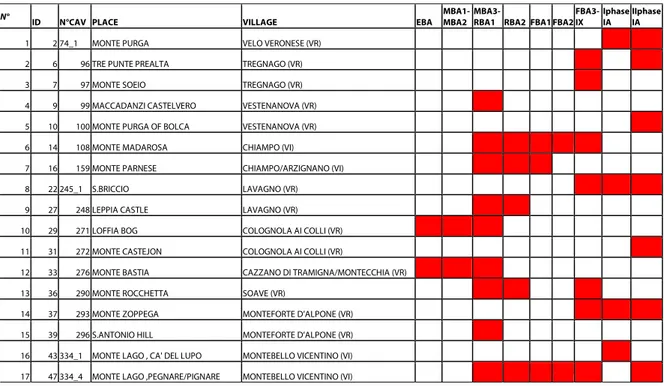
N°
ID N°CAV PLACE VILLAGE EBA
MBA1-MBA2
MBA3-RBA1 RBA2 FBA1 FBA2 FBA3- IX Iphase IA IIphase IA
1 2 74_1 MONTE PURGA VELO VERONESE (VR) 2 6 96 TRE PUNTE PREALTA TREGNAGO (VR) 3 7 97 MONTE SOEIO TREGNAGO (VR) 4 9 99 MACCADANZI CASTELVERO VESTENANOVA (VR) 5 10 100 MONTE PURGA OF BOLCA VESTENANOVA (VR) 6 14 108 MONTE MADAROSA CHIAMPO (VI) 7 16 159 MONTE PARNESE CHIAMPO/ARZIGNANO (VI) 8 22 245_1 S.BRICCIO LAVAGNO (VR) 9 27 248 LEPPIA CASTLE LAVAGNO (VR) 10 29 271 LOFFIA BOG COLOGNOLA AI COLLI (VR) 11 31 272 MONTE CASTEJON COLOGNOLA AI COLLI (VR)
12 33 276 MONTE BASTIA CAZZANO DI TRAMIGNA/MONTECCHIA (VR) 13 36 290 MONTE ROCCHETTA SOAVE (VR)
14 37 293 MONTE ZOPPEGA MONTEFORTE D’ALPONE (VR) 15 39 296 S.ANTONIO HILL MONTEFORTE D’ALPONE (VR) 16 43 334_1 MONTE LAGO , CA' DEL LUPO MONTEBELLO VICENTINO (VI) 17 47 334_4 MONTE LAGO ,PEGNARE/PIGNARE MONTEBELLO VICENTINO (VI)
Tab. I: List of settlements with their chronological phases (EBA: Early Bronze Age; MBA1-MBA2: Middle Bronze Age 1 – Middle Bronze Age 2; MBA3-RBA1: Middle Bronze Age 3 – Recent Bronze Age 1; RBA2: Recent Bronze Age 2; FBA1: Final Bronze Age 1; FBA2: Final Bronze Age 2; FBA3-IX century BC: Final Bronze Age 3 – IX century BC; I phase IA: First
phase of Iron Age; II phase of IA: Second phase of Iron Age).
Tab. II: Histogram representing both the presence and the persistence of settlements in each chronological phase.
Histogram of settlements 0 1 2 3 4 5 6 7 8 9 10 MBA1-MBA2 MBA3-RBA1
RBA2 FBA1 FBA2 FBA3-IX cent. I phase IA II phase IA chronological phase N ° abandonments total activations in continuation
5 Fig. 2: Distribution map of settlements of all chronological phases.
VARCOST ANALYSIS: THE BUFFER AREAS OF SETTLEMENTS
The vectorial points representing ancient settlements were imported in IDRISI GIS™ and converted from vectors to raster files. There is no information about the size of these protohistoric settlements, for this reason in order to consider the archaeological location not as a simple point (10 per 10 meters, DTM resolution) but as a more realistic buffer area that takes into account the morphology of the context, it was conventionally decided to deal the cost of moving as a decisive factor for the evaluation of the
settlement size. Indeed, the morphology of the context and the difficulty to face it could have really affected the possible extent of a site in the past.
First of all, the anisotropic and topographic variables of slope and aspect are calculated from the DTM. The Varcost operator permits to calculate an energetic cost surface in which each pixel expresses a cost value that increases together with both the distance from the start point and the slope values. For this operation it is necessary to have:
1- a Source image: a raster image in which the contemporaneous settlements are spread. They are identified by a number code different from zero on a raster surface in which the rest of pixels have a value of zero;
2- an Anisotropic friction surface: frictional elements that have different effects in different directions. In this case, the slope image (friction that affects the cost of human movement) accompanied by an aspect image (friction direction image which represents in azimuths the direction of movement that would incur the greatest cost);
This spatial analysis looks like the Site catchment analysis developed by Higgs and Vita-Finzi (1970) used to visualize the catchment of resources exploited by a settlement for its subsistence. The main principle of this theory is that an ancient settlement tends to select a suitable position to exploit the surrounding environment in the least wasteful way.
Fig. 3: Varcost image of all settlements. Each pixel receives a Cost value according to the indexes of the coloured
palette: each pixel has a cost value that depends on both the distance from the start point and the slope of the location. The catchment cost area of each settlement ends when it meets the same cost value belonging to the
7 The principle used here is the same but, on the other hand, the variables measured are different: the site catchment analysis considers the presence of resources which decreases as the distance from the site increases, instead the Varcost analysis measures the energetic cost which raises as the distance from the site increases because more and more distances and slopes must be faced when a person moves to get a particular target.
An important point that should be highlighted is that the Varcost analysis can also deal with the isotropic friction of land use (CASAROTTO, DE GUIO, FERRARESE 2009) but for the buffer areas of settlements it is
believed that morphological factors are sufficient to hypothesize the possible size of a settlement. Therefore it was assumed that the size of an ancient settlement is directly proportional to the topographic conditions of the context, thus to obtain the buffer areas we conveniently decide to fix the energetic cost due to move from each settlement to any direction at “30” cost units. This value, in optimal slope conditions, corresponds to about 300 meters in a straight line.
In this way it was possible to get irregular masks which account of topography of the location and represent the possible settlement extension. These buffer areas will be used to calculate some environmental characteristics of the location such as the slope average, the altitude average, the solar radiation average, the hypotetical land use, the intervisibility and the morphology of the location.
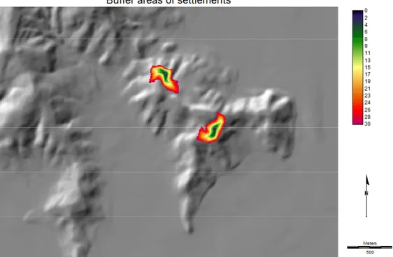
Fig. 4: Buffer areas of settlements representing the possible size of a settlement according to the energetic cost due to face the topographic conditions of the context when someone spends “30” cost units to move from each
settlement to any direction.
DECISIONRULE:THEVARIABLESOFTHEMULTICRITERIAANALYSIS
The predictive model presented below can be conceptualised as “a form of what planners call location – allocation analysis, in which the object is to allocate suitable locations to specific types of human activities, and in which the criteria of suitability are derived by location analysis - the generation of behavioural rules from a set of observations about how people actually behave or have behaved in the past” (VAN LEUSEN,KAMERMANS 2005,p.26).
Before planning a predictive model that visualizes the most siutable locations to be inhabited in the past, the decision rule must be formulated. It is used to order in a gerarchic scale the supposed decision-making options according to the knowledge base and the ancient decisor’s preferences. The decision rule describes the conditions by which a particular location is considered appropriate for the presence of unknown settlements. This rule is based on some environmental variables that could have affected the human behaviour and oriented the choice of a location. These criteria have been selected after the study of the bibliographic information, and above all after the empirical observations on a pattern of known settlements in a GIS setting: “if a precise and accurate description of the known sample can be made, so the implicit argument goes, then we will automatically have a precise and accurate prediction of the parent population of sites” (VAN LEUSEN,KAMERMANS 2005,p.31). The criteria used to predict the presence of
new archaeological sites are: longitude (“X”), latitude (“Y”), altitude average (“Z”), slope average, intervisibility, land use, solar radiation average, distance from water, euclidean distance from the nearest neighbour archaeological site, cost distance from the nearest neighbour archaeological site and morphology of the location.
GIS technology is able to translate the environmental variables in quantitative ones, so each variable can be converted in a raster image and subjected to statistical analysis for a better understanding of the logic of the settlements distribution. Then each variable is reclassified with new values of suitability, on a scale of 0 to 10 according to the previous statistical analysis, that represent the possible strategy followed by the ancient social actors to found a settlement. Following this process, Criterion maps (DI ZIO,BARNABEI
2009) are obtained and finally will be overlaid and standardized in an unique plausibility value. Even though the values of suitability used to reclassified each variable are suggested by statistics, they strongly depend on the operator’s personal judgement. In addition, the choice of the environmental variables is subjective and resulting from the availability of information and the actual research stage in the study area. Also the weight given to each variable is subjective: so we can understand that the potentially settled zones depend on the criteria the operator considers most important in location-allocation strategies.
The Criterion maps of each environmental variable are calculated for each chronological phase but for the Early Bronze Age, the Middle Bronze Age 1 and 2, and for the Final Bronze Age 2 the number of known settlements is insufficient (only two settlements for each phase) to return effective statistics. The Criterion maps and the next Settlement plausibility maps can be elaborated as long as the settlement density is high enough, because only in this way we can obtain reliable statistics. For this reason both the Criterion maps and the Settlement Plausibility maps of the chronologial phases listed upon, will not be calculated and it was decided to focus on the remaining ones.
Longitude and latitude
The study area is shared in three bands scanned every 10,000 meters in longitude and latitude. The spatial distribution of existing sites is controlled for each chronological phase both in longitude and in latitude to establish a set of presence percentages of known settlements within the X bands and Y bands. In the next step each band receives a suitability value, according to the previous statistics, which is used in IDRISI GIS™ to reclassify the study area and obtain Criterion maps of longitude and latitude variables.
We decided to consider these two variables because, in the same topographical conditions the majority of settlements tends to be located in the eastern part of the study area. If the logic of this spatial distribution was not a random one, but rather the result of a planning influenced by the presence of some kind of cultural elements (such as a political boundary), it would be important to take the longitude and the latitude into account.
Altitude average
The DTM is shared in a number of altimetric bands according to Leonardi G. (2006, p. 437) up to 1200 m a.s.l. (after this altitude, regular bands of 400-meter height are considered):
I) band from 0 m to 150 m a.s.l., II) band from 150 m to 300 m a.s.l., III) band from 300 m to 600 m a.s.l., IV) band from 600 m to 900 m a.s.l., V) band from 900 m to 1200 m a.s.l., VI) band from 1200 m to 1600 m a.s.l., VII) band from 1600 m to 1966 m a.s.l. (highest altitude of the DTM).
This particular scanning of the altimetric scene refers to a rational organization of the territory based on both productive capabilities and availability of resources of the different eco-zones.
For each chronological phase the spatial distribution of existing sites is controlled to establish a set of presence percentages of known settlements in each altimetric band. Then each altimetric band receives a suitability value, considering the previous statistics, that reflect the aptitude (regarding the altitude) to set up a coeval site. We must remark that for the computation of the Altitude average we consider the buffer areas of settlements. The majority of known settlements tends to be located from 0 m to 600 m a.s.l. during the Middle Bronze Age 3 and Recent Bronze Age 1, from 150 m to 600 m a.s.l in the Recent Bronze Age 2, in the Final Bronze Age 1 and in the Final Bronze Age 3 and IX century BC, from 150 m to 300 m a.s.l. in the First phase of Iron Age and from 150 m to 900 m a.s.l. in the Second phase of Iron Age. These altitude bands seem the most suitable to found a settlement, thus they receive a higher value of suitability than the others.
IDRISI GIS™ can reclassify the DTM and obtain Criterion maps of each phase according to the altitude averages which are more or less likely for the presence of a new archaeological site.
9 Fig. 5: DTM of the study area (10 per 10 meters resolution). Raster image of Altitude calculated in m a.s.l.
Slope average
For each chronological phase the anisotropic friction surface of slope made previously is divided into a number of degree bands. The spatial distribution of existing sites is therefore controlled in order to establish a set of presence percentages of known settlements in each degree band. Afterwards all the degree bands receive some suitability values, considering the previous statistics, in order to reflect the aptitude (regarding the slope) to set up a coeval site. The Slope average is calculated in the buffer areas of settlements. Independently of the chronological phase, the majority of known settlements tends to be located in zones with a slope angle from 0° to 20°. This degree band seems the most suitable to found a settlement, thus it receives a higher value of suitability than the others.
This way IDRISI GIS™ can reclassify the Anisotropic friction surface of slope and obtain Criterion maps of each phase according to the slope averages which are more or less likely for the presence of a new archaeological site.
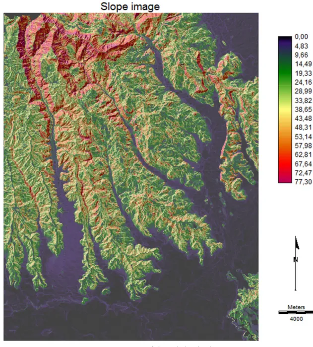
Fig. 6: Raster image of Slope calculated in degrees.
Solar radiation average
In ancient times the solar exposition of a site had an important role in the allocation choice: zones which were most sunny took advantages of more hours of daylight, such as the heating, the prolonged visibility and more productive agricultural and farming activities.
In ArcGIS 9.3™ there is a specific algorithm to calculate the power of solar radiation in any part of the study area. To each pixel of the DTM a solar power index is given, it indicates the number of Watt per square meter. These power indexes are measured for “special days”, i.e. for the solstices (solar extreme situations) and for the equinoxes (solar intermediate situations). For known settlements there is a strong similarity between the solar radiation average of solstices and equinoxes, therefore it was decided to consider the raster image of solar radiation in equinox days as an average situation of the daily power of the solar radiation. The raster image of the solar radiation is therefore divided into a number of solar power bands. For each chronological phase the spatial distribution of existing sites is controlled to establish a set of presence percentages of known settlements in each solar power band. Afterwards each of these receives a suitability value, considering the previous statistics. Solar radiation average is always calculated in the buffer areas of settlements. Independently of the chronological phase, the majority of known settlements tends to be located in zones with a solar radiation average from 2600 W/m2 to 2900 W/m2. This solar power band seems the most suitable to found a settlement, thus it receives a higher value of suitability than the others.
11 In IDRISI GIS™ the image of solar radiation is reclassified to obtain Criterion maps of each phase according to the solar radiation averages which are more or less likely for the presence of a new archaeological site.
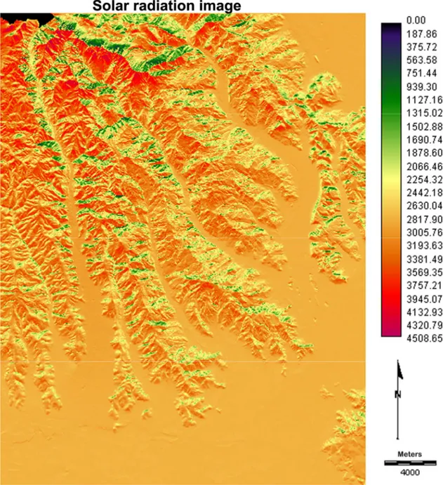
Fig. 7: Raster image of Solar Radiation calculated in Watt per square meter.
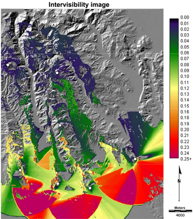
Intervisibility
The Viewshed Analysis tool produces a spatial simulation of what could be seen from an ancient settlement. It measures the extent of human range of vision from a particular source point to any direction in the space, considering both the altitude of the observation point and the altitude of each pixel of the DTM. This way it is possible to make a complex simulation of the relationship between the morphology of the landscape and the settlement systems (FORTE 2000, pp.100-101). This is a fundamental
analysis to study the ancient landscape and to re-enact its possible perception.
Viewshed analysis calculates the view catchment area of a site but it also highlights the view interactions between a set of coeval settlements: in this case of study, settlements of each chronological phase are considered as view sources in which there is an hypothetical 1.70 meter tall viewer who is looking at the landscape, using a 8000 meters view radius and a 360° view angle.
For the computation of the Intervisibility images the buffer areas of settlements are considered: the GIS assigns to each pixel of the DTM a value that is proportional to the number of points of the buffer areas
from which that pixel is visible. The cumulative amount of visibility can be valued for all the settlements of each chronological phase and it focuses on the possible strategy used to control the territory.
In this case of study it is supposed that settlements, many of which are also fortified (CAPUIS et al. 1990), held a strategic position in the control of the territory, and were mutually linked in a network of sites dependent on a single territorial and social organization which was wider and more complex (LEONARDI
2006), as well as constituted by other peripheral areas and central places in the plain. Indeed they probably had to defend a marginal area in which there was a wide potential exposition to conflicts among different territorial and political systems (LEONARDI 1992c). For these reasons it was assumed that
an unknown archaeological settlement should be easily visible from the coeval ones and so it should be positioned in portions of the landscape which are ideally viewed by all settlements of its chronological phase. Intervisibility images are reclassified with dichotomous values of “1” to those cells which are visible and “0” to the invisible ones.
Fig. 8: Raster image of Intervisibility of the Second phase of Iron Age settlements.
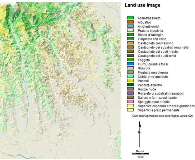
Land use
The land use data derive from the Land use map 2009 of Veneto Region: no information were available about the ancient situation of the land use, therefore it was necessary to refine this map and reclassify some land use classes such as actual residences, infrastructures, parks, orchards or roads which did not
13 exist in protohistiric times. These critical zones are joined with the nearest ones which are characterised by land use classes that could be reliable also for the Bronze and the Iron Ages. Through an overlay operation in IDRISI GIS™, it is possible to multiply the Land use image with the buffer areas of settlements and then a query of cross tabulation can establish on what land use classes the known settlements bear. The typical land use classes found in correspondence to settlements are bushes, prairie, wood, chestnut trees, beech trees, oak trees, pasture land and grass. For each buffer area of settlements, percentages of land use classes are calculated and then values of suitability, which reflect the aptitude (regarding the type of land use) to set up a coeval site, are given to them.
It was evaluated that a precise strategy seems to exist, in fact the majority of settlements is located on prairie. However this constant could depend on the facility for the modern researchers to find an archaeological site in a prairie land rather than others such as wood.
Such Land use map has to be used carefully because it gives information about the actual situation and so just an hypothetical ancient landscape can be imagined. Indeed it is a not much informative attribute because there is a missing link between the information available and the information necessary.
Fig. 9: Raster image of hypotetical Land use.
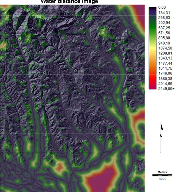
Distance from water
An important factor that could have influenced the settlement location choice is the distance from the nearest source of water. However it can sometimes happen that the demand to stay in proximity of water sources opposes the contemporary defensive criterion to stay on the peaks of hills.
In this predictive model was considered both the distance from flows and sources using the analysis tool of proximity called “Near” in ArcGIS™ and the distance operator called “Distance” in IDRISI GIS™.
The spatial distribution of existing sites is controlled in order to establish a set of presence percentages of known settlements in relation to the distance from water. Afterwards the raster image of the distance from water receives some suitability values, considering the previous statistics, in order to reflect the aptitude (regarding the distance from water) to set up a coeval site. The majority of known settlements tends to be located from 50 m to 400 m far from the nearest source of water during the Middle Bronze Age 3 and Recent Bronze Age 1, in the Recent Bronze Age 2 and in the Final Bronze Age 1, from 200 m to 900 m far in the Final Bronze Age 3 and IX century BC, from 600 m to 1000 m farduring the First phase of
Iron Age and from 200 m to 500 m far in the Second phase of Iron Age. These distances from water seem the most suitable to found a settlement, thus they receive a higher value of suitability.
The image of the distance from water was reclassified to obtain Criterion maps of each phase according to the distances which are more or less likely for the presence of a new archaeological site.
Fig. 10: Raster image of Distance from water calculated in meters.
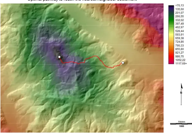
Euclidean distance and Cost distance from the nearest neighbour archaeological site
It was tried to think about the territorial management and competence of settlements in Bronze and Iron Ages by measuring the distance from the nearest neighbour. This distance probably played a leading role in the social interactions between coeval settlements, thus both the Euclidean distance and the Cost distance was considered. The former is obtained by using the analysis tool of proximity called “Near” in ArcGIS™ and the distance operator called “Distance” in IDRISI GIS™, the latter considers the topography of the context and indicates the optimal pathway to reach the nearest neighbour point (archaeological site). This path is the least expensive because follows the gentlest slopes and the shortest distance, it is obtained by using the Varcost image and the “Pathway” tool in IDRISI GIS™.
The spatial distribution of existing sites is therefore controlled in order to establish a set of presence percentages of known settlements in relation to the Euclidean distance and Cost distance from the nearest neighbour archaeological site. Afterwards the two raster images of distance from the nearest neighbour receive some suitability values, considering the previous statistics.
There are no significant constants regarding the variable of the Euclidean distance but when one considers the Cost distance, the majority of known settlements tends to be located from 200 cu (cost unit)
15 to 700 cu far from the nearest neighbour settlement during the Middle Bronze Age 3 and Recent Bronze Age 1, from 400 cu to 800 cu far in the Recent Bronze Age 2, from 500 cu to 700 cu far in the Final Bronze Age 1, from 200 cu to 300 cu far in the Final Bronze Age 3 and IX century BC, from 200 cu to 700 cu far in the First phase of Iron Age and from 400 cu to 700 cu farduring the Second phase of Iron Age. These Cost distances from the nearest neighbour archaeological site seem the most suitable to found a settlement, thus they receive a higher value of suitability.
Fig. 11: Optimal pathway which connects the settlement of “Monte Madarosa” with its nearest neighbour settlement of “Monte Parnese”.
Morphology of the location
This environmental variable seems the most significant in the spatial pattern of ancient settlements. The majority of them, independently of the chronological phase they belong to, rises on some kind of ridge that is the best morphological condition to control the territory.
Morphology image is an automatic and semi-automatic reclassification of the DTM depending on slope and curvature derivatives, which were calculated using a kernel of 3 per 3. Three operators were used, “Topographic modelling”, “K-means” and “Topographic feature” of ENVI™, to obtain a map with five morphological classes: ridge, hillside, channel, plain and ravine.
The spatial distribution of existing sites is controlled in order to establish a set of presence percentages of known settlements in relation to the morphological condition on which they lie. Afterwards, each morphology class receives a suitability value considering the previous statistics. The “ridge” seems the most suitable morphological class to found a settlement, thus it receives a higher value of suitability than the others.
THE WEIGHT OF VARIABLES: PAIRWISE COMPARISON TECHNIQUE
There are many techniques to assign weights to a linear combination of variables, the majority of which are based on judgments of experts who have an exhaustive anthropological, archaeological and historical knowledge about the social dynamics occurred in a study area. It was decided to use the Pairwise Comparison technique devised by the American mathematician Thomas Lorie Saaty (SAATY 1980), which
is an integral part of many GIS softwares (EASTMAN 2006). The Pairwise comparison in IDRISI GIS™ uses a
scale from 1/9 to 9 which expresses the relative importance of the first variable compared to the second one.
Fig. 12: Raster image of Morphology.
By comparing all the possible pairs of variables, the values of importance are organized in a matrix using the “Weight” operator of IDRISI GIS™ which can calculate absolute weights expressing the different grade of influence they play in a decision making-process. The fundamental condition is that the sum of weights must be “1”:
Longitude: 0,0135 Latitude: 0,0135
Altitude average: 0,2117 Slope average: 0,1632
Solar radiation average: 0,0771 Intervisibility: 0,0199
Land use: 0,1107
Distance from water: 0,0949
Euclidean distance from the nearest neighbour: 0,0461 Cost distance from the nearest neighbour: 0,0449 Morphology of the location: 0,2045
It is possible to note that greater importance is given to the topographic factors of altitude average, morphology of location and slope average and, in the second place, resources as water and land use. The weight of environmental factors depends on the personal interpretation of statistics, therefore it is quite subjective and related to the archaeological, anthropological and historical expertise of the researcher.
17
SETTLEMENT PLAUSIBILITY MAPS
Multicriteria decision making is a set of systematic procedures for analyzing complex decision problems, and can be applied to archaeological predictive modelling because it is concerned with complex decision problems faced both in the past (e.g., settlement choice) and today (e.g., spatial planning). In this predictive model the goal of the decision maker is to identify the optimal locations for ancient settlements according to a set of evaluation criteria (called objectives or attributes) (VAN LEUSEN,KAMERMANS
2005, p. 64 ; VERHAGEN 2007, p.72).
The MCE (Multi Criteria Evaluation) of IDRISI GIS™ can manage any GIS surface considering it an expression of information about a variable for every spatial location in the dataset. For raster data this information is expressed as a value for every point on a regular grid. MCE combines Criterion maps according to their weights and standardizes them in an unique scale of plausibility values by using the Weighted Linear Combination (EASTMAN 2006). The result is a raster image which continuously charts the settlement probability all over the study area and gives a suitability value to each pixel, according to this predictive formula:
∑
==
n jWjXij
Pi
1where “n=11” is the number of input criteria, “i” is the location of pixel, “X” indicates the value assumed by criterion “j” in pixel “i”, “W” is the weight of the criterion “j”, and “P” is the plausibility value in the pixel “i” (DI ZIO,BERNABEI 2009, p. 323). The resulting image is a map of decision alternatives, and the decision maker’s preferences will probably orient to those locations with a high settlement plausibility value.
Fig. 13: Settlement Plausibility map for the Middle Bronze Age 3 and for the Recent Bronze Age 1, calculated with the MCE in IDRISI GIS™. Each pixel has a value of suitability from 0 to 7 according to a palette from white to dark red.
TESTING MODEL
It must be critically said that some environmental factors could effectively have influenced the ancient human behaviour and so the distribution of existing sites; however it is possible that they also affect the behaviour of the modern researcher who decides to survey those locations which are now easier to reach, cross and see. If it was, the known settlements distribution would be a simple random one and not the effect of particular social dynamics and location-allocation strategies. One way to assess the quality of a model is to test it. Generally, any useful model must suggest at least one hypothesis that allows the model builder to design a test experiment. In this case of study two tests are carried out in order to evaluate the reliability of the predictive model and to reduce bias.
The first test: “spread finds” mapping
The category of archaeological sites called “spread finds” is an archaeological location attested by more or less scholarly educated operators but not systematically investigated by archaeological surveys or excavations (CAPUIS et al. 1990). Nevertheless, they could be probable settlements of some phases of Bronze and Iron Ages. By testing this hypothesis their positions are intersected with the Settlement Plausibility maps: if the locations of “spread finds” overlap high plausibility values, the fact would give reason to these remains (that could at this point be interpreted as possible settlements) and would somehow test the functionality of this predictive model.
The majority of “spread finds” effectively falls in high values of settlement plausibility.
Spread finds Tot. high P medium-high P medium P low P
Middle Bronze Age 3 - Recent Bronze Age 1 11 9 1 0 1
Recent Bronze Age 2 5 2 3 0 0
Final Bronze Age 1 3 2 1 0 0
Final Bronze Age 3 – IX century BC 1 1 0 0 0
Second phase of Iron Age 4 3 0 0 1
Tab. III: Spread finds attested in some phases of Bronze Age and Iron Age (i.e. Middle Bronze Age 3 - Recent
Bronze Age 1, Recent Bronze Age 2, Final Bronze Age 1, Final Bronze Age 3 – IX century BC and Second phase of Iron Age) and their Plausibility (P) values
The second test: the second operator’s Settlement Plausibility map
It was already underlined that the key problem of this model is the subjectivity of both the choice and the weight of criteria employed. In order to control and limit this subjectivity, reveal weaknesses and contribute to the advancement of theory the interpretations obtained so far are compared with a second operator’s ones. The researcher uses his own expertise and decides to consider seven criteria (altitude average, slope average, intervisibility, solar radiation average, land use, cost distance from the nearest neighbour archaeological site and morphology of the location). Then he reclassifies the variables with Fuzzy tool of IDRISI GIS™ in order to obtain Criterion maps and to weigh them personally. He autonomously produces another Settlement Plausibility map of the Middle Bronze Age 3 and Recent Bronze Age 1 with MCE of IDRISI GIS™.
Finally the plausibility values of the second operator’s map are compared with the plausibility values of the first operator’s one. The results are absolutely comparable and confer a higher degree of confidence on the method. The distribution of “spread finds” is controlled here too: 80% falls in high values, 10% in medium-high and just 10% in low values of plausibility.
19
Figure 14: Settlement Plausibility map for the Middle Bronze Age 3 and for the Recent Bronze Age 1 calculated by a
second operator (Francesco Ferrarese). This map derives from MCE in IDRISI GIS™ using seven variables reclassified with fuzzy tool. Each pixel has a value of suitability from 0 to 255 according to a palette from green to purple.
FUZZY ANALYSIS
Fuzzy logic is a departure from classical binary Boolean logic, in which a variable can assume only two value “1” or “0”, “true” or “false” and so on. It is easy to understand why the Boolean logic is quite imprecise when the reality must be represented: in the real life there are many intermediate and uncertain situations which can hardly be translated with strict Boolean values. The fuzzy logic would like to reproduce the way of thinking of human brain that usually expresses concepts such as “almost true” or “partially false” and so on. It uses a continuous range of true values (from 0.0 to 1.0 or from 0 to 255) rather than strict binary (1 or 0) decisions and assignments. The Fuzzy logic measures uncertainty by assigning a set of probabilities to a set of possibilities. In this way the Fuzzy logic can also deal vague or missing data, such as many archaeological information, because it can incorporate the uncertainty in the prediction. For this reason the Fuzzy analysis can build a bridge between expert’s judgement and quantification, uncertain data and representation.
The variables are reclassified again but now using the Fuzzy tool of IDRISI GIS™ in order to obtain Criterion maps. Then Settlement plausibility maps of the rest of chronological phases are calculated using the MCE technique. In spite of the fact that now variables are reclassified with a continuous range of values (from 0 to 255) instead of a discrete one (from 0 to 10), the new Settlement plausibility maps respect the general distribution of previous settlement plausibility.
CONCLUSIONS
This predictive model tries to better understand the complex interaction between natural and social system in the past. It represents an actor in a cognitive process and his or her ability to make a settlement decision is the consequence of their perception of the landscape. Beyond environmental variables, some perception factors could influence the settlement location choice, such as the viewshed and the proximity to both resources and coeval settlements, but it must be said that other qualitative landscape features could affect human perception and the political organization of the territory; at this moment, we cannot predict the effects of those ones on ancient behaviour.
However, the results obtained so far seem really comforting, even though there are some intrinsic limitations in this predictive model that must be taken into consideration: some of these are practical in nature (i.e. do we really have the information to predict the archaeological evidence?) and theoretical (i.e. did people choose their settlements based on environmental variables only?). Predictive modelling is still a controversial issue and it is often criticised for the use of incomplete archaeological data sets and also for the predominant use of environmental input variables as archaeological sites predictors rather than cultural factors (VERHAGEN 2007;WHEATLEY,GILLINGS 2002).
Figure 15: Reclassification of the Settlement Plausibility map for the Middle Bronze Age 3 and for the Recent Bronze
Age 1. This figure shows locations which must be surveyed: they are classified in three classes depending on the area/perimeter ratio of irregular polygons formed by adjoining pixels. The higher the ratio is, the more suitable the
21 For example in this predictive model is not considered the influence of qualitative landscape features that can be interpreted as having cultural significance. They can attract or push away the human behaviour, such as territorial boundaries, cult places, necropolises. Unfortunately at this moment in Eastern Lessinia, historical and anthropological information are insufficient to deal and weigh cultural variables, therefore we are unable to translate them in continuous and quantitative raster decision surfaces.
Nevertheless the two tests validate the quality of this predictive method that could be also reproduced in any other study area and used in archaeological heritage management: it gives a preliminary presence probability of archaeological sites and it can direct archaeological surveys in “terra incognita”, reducing cost and time of ground truth.
Predictive modelling also stimulates the eye thinking and the confidence with the examined territory grows up, in this way, the researcher develops unexpected hypotheses about ancient location-allocation strategies which are useful to better understand the human behaviour in the past.
FUTURE RESEARCH PERSPECTIVES
The archaeological research in Eastern Lessinia was inertial and anchored to results obtained by scholars about thirty years ago. By implementing this predictive model, it would be possible to start a systematic archaeological survey oriented to high plausibility locations. However, before the activation of an operational research, the predictive model must be improved. The distribution of known settlements in Bronze and Iron Ages suggest a precise strategy for the organization of the territory. In fact archaeological sites are usually located on ridge, in gentle slopes at altitudes from 150 m to 600 m a.s.l, , with a solar radiation included from 2600 to 2900 W/m2 (average values of solar radiation in the study area) and in prairies. Some fly through simulations were conducted in IDRISI GIS™ setting, and they permit to realize that the majority of settlements puts on high plausibility values but they are surrounded by medium and low plausibility values. It probably means that people preferred those locations which facility the control of the territory but, at the same time, they are also difficult to reach. This new cultural variable could be introduced in the predictive model and it would permit to reduce further more the high settlement plausibility locations that have to be surveyed.
Figure 16: This picture is extracted from a virtual Fly through simulation in IDRISI GIS™ setting. It represents the
Settlement Plausibility map of Eastern Lessinia (Verona and Vicenza, Northeastern Italy) for the Middle Bronze age 3 and the Recent Bronze age 1. The blue spots indicate the locations of known settlements.
Another cultural variable should be added: some known settlements persist for a very long period, on the other hand, some others last for just a chronological phase. They evidently had a different influence in political and social dynamics, for this reason it seems necessary to think about a way to build and manage a rank rule of settlements. The survival rate itself could be therefore assumed as a potential explanatory variable (DE GUIO 1985a).
Finally it will be obtained an absolute signature of plausibility that could be automatically recognized all over the study area and verified only throughout archaeological survey.
The real importance of this predictive model is its replicability anywhere, therefore in other contexts and for other chronological overviews. In addition, the possibility to have a wider set of informative data could make the model even more powerful.
REFERENCES
ASPES A.,a cura di,1984,Il Veneto nell’antichità: preistoria e protostoria, vol. I-II, Verona, Banca popolare di Verona.
ASPES A.,a cura di,2002, Preistoria veronese. Contributi e aggiornamenti, MemVerona, 2° Serie, n. 5.
BAGOLAN M.,LEONARDI G. 1999, Montebello vicentino e la facies culturale veneta nel tardo bronzo, Archeologia
delle Alpi, 5, pp. 213-258.
BAGOLAN M., LEONARDI G. 2000, Il Bronzo Finale nel Veneto, in HARARI M., PEARCE M., a cura di, Il
Protovillanoviano al di là e al di qua dell’Appennino, Atti della giornata di studio, Pavia, Collegio Ghislieri, 17 giugno 1995, Como, pp. 13-44.
BALISTA C.,LEONARDI G.1985, Hillslope evolution: pre and protohistoric occupation in the Veneto, in The Third
Conference of Italian Archaeology, BAR Internat. Series, 243, Cambridge, pp. 135-152;
BALISTA C., DE GUIO A., LEONARDI G., RUTA SERAFINI A. 1982, La frequentazione protostorica del territorio
vicentino: metodologia analitica ed elementi preliminari di lettura interpretativa, in DArch, 2, pp. 113-136. BIANCHIN CITTON E.1984, Il Bronzo finale, in ASPES A., a cura di, Il Veneto nell'antichità. Preistoria e protostoria, II, Verona, Banca popolare di Verona, pp. 617-630.
BIANCHIN CITTON E.1999, Il Veneto Orientale tra Età del Bronzo medio-recente e prima Età del Ferro, in ADRIANO
MAGGIANI,a cura di, Protostoria e Storia del “Venetorum angolus”, AttiSEI XX, Pisa, Roma, pp.31-46.
BIANCHIN CITTON E.2003, Le origini: la formazione della civiltà veneta nell'età del bronzo finale (XII-X secolo a.C.), in MALNATI L.,GAMBA M., a cura di, I Veneti dai bei cavalli, Treviso, Canova, pp. 23-31.
BISAZZA A.,FERRARESE F.,MOZZI P.,NINFO A.2009, La valutazione della vulnerabilità idraulica in un’area di pianura alluvionale della provincia di Padova, mediante “Multi criteria evaluation”, in AGNESI V.,a cura di, Ambiente geomorfologico e attività dell’uomo risorse, rischi, impatti, Atti del II Convegno Nazionale A.I.Geo, Torino, 28-30 marzo 2007, Società Geografica Italiana, Roma, pp. 99-111.
CAPUIS L.,DE GUIO A.,LEONARDI G.1984, Il popolamento in epoca protostorica, in BOSIO L.,a cura di,Misurare la terra: centuriazione e coloni nel mondo romano. Il caso veneto, Catalogo della Mostra, Modena, Panini Franco Cosimo editore, pp. 38-52.
CAPUIS L.,LEONARDI G.,PASAVENTO MATTIOLI S.,ROSADA G., a cura di, 1990, Carta archeologica del Veneto, Vol. II, Foglio 49, Modena, Panini Franco Cosimo editore, pp. 95-176.
CAPUIS L.2004, I Veneti, Milano, Longanesi &C..
CASAROTTO A.2008, ACTION GIS: modelli pre-dittivi e post-dittivi nell'analisi del movimento. Il caso di studio
archeologico della Val d'Alpone (VR), Bachelor’s dissertation, supervisor De Guio A., co-supervisor Ferrarese F., Università degli Studi di Padova.
CASAROTTO A.,DE GUIO A.,FERRARESE F.2009, ACTION GIS: un modello predittivo del movimento antropico in un
paesaggio antico. Il caso di studio archeologico della Val d’Alpone (VR), Archeologia e Calcolatori, 20, Firenze, pp. 291-307.
CASAROTTO A.2010, Archeologia Predittiva: un modello GIS multicriterio e multiobbiettivo per la localizzazione
di siti protostorici in Lessinia Orientale, Master’s dissertation, supervisor De Guio A., co-supervisors Leonardi G., Ferrarese F., Università degli Studi di Padova.
CHAPMAN H. 2006, LANDSCAPE ARCHAEOLOGY AND GIS,UNITED KINGDOM,THE HISTORY PRESS LTD
DE GUIO A.1983, Strategie locazionali e diacronia: linee di un approccio analitico, in AA.VV., Problemi storici ed archeologici dell’Italia nordorientale e delle regioni limitrofe dalla preistoria al medioevo, Atti del Convegno, Trieste, 28-30 ottobre 1982, Civici Musei di Storia ed Arte di Trieste, Quaderno XIII, 1, pp. 201-223.
DE GUIO A. 1985a, Archaeological applications of survival analysis,in VOORIPS A.,LOVING S.H. (eds.), To pattern the past, P.A.C.T, 11, Souvain, pp.361-381.
DE GUIO A. 1985b, Archeologia di superficie ed archeologia superficiale, QAV, I, pp.176-184.
DE GUIO A.,EVANS S.P.,RUTA SERAFINI A.1986, Marginalità territoriale ed evoluzione del “paesaggio di potere”: un caso di studio in Veneto, in QAV, II, pp. 160-172.
23 DE GUIO A. 1991, Alla ricerca del potere: alcune prospettive italiane, in HERRING E.,WHITEHOUSE R.,WILKINS J. (eds.), Paper of the fourth conference of Italian archaeology: the archaeology of power, Part 1, London, Accordia Research Centre, pp. 154-192.
DE GUIO A.1992 , “Archeologia della complessità” e calcolatori: un percorso di sopravvivenza fra teorie del caos, attrattori strani, frattali e...frattaglie del postmoderno, in BERNARDI M., a cura di, Archeologia del
paesaggio, I, Firenze, Ed. All’Insegna del Giglio, pp. 305-389.
DE GUIO A.1994, Dal bronzo medio all’inizio dell’età del ferro, in AA.VV., Storia dell’Altipiano dei Sette Comuni,
Vicenza, Banca Popolare Vicentina, pp.157-177.
DE GUIO A. 1995, Surface and subsurface: deep ploughing into complexity, in HENSEL W.,TABACZYNSKI S.,
URBANCZYK P., Theory and practice of archaeology research, II, Institute of Archaeology and Ethnology,
Committee of Pre and Protohistory Sciences, Polish Academy of Sciences, Warszawa, pp. 329-414.
DE GUIO A. 1996, Archeologia della complessità e pattern recognition di superficie, in MARAGNO E., a cura di, La
ricerca archeologica di superficie in area padana, Stanghella, Padova, Linea AGS Edizioni, pp. 275-313. DE GUIO A. 1997a, “Landscape Archaeology” e impatto archeologico: una rivoluzione annunciata, in QUAGLIOLO M., a cura di, La gestione del patrimonio culturale. Cultural Heritage management. Lo stato dell’arte, Roma, DRI - Ente Interregionale, pp.50-67.
DE GUIO A.,CATTANEO P.1997b, “Dirt roads to Brendola”: le strade preistoriche di Soastene-Brendola (Vicenza), in QAV, XIII, pp. 168-182.
DE GUIO A. 2000, Power to the people? “Paesaggi di potere” di fine millennio, in CAMASSA G.,DE GUIO A., VERONESE F.,a cura di, Paesaggi di potere: problemi e prospettive, Roma, Quasar, pp. 3-29.
DE GUIO A. 2001, “Superfici di rischio” e C.I.S.A.S. se lo conosci, non lo eviti, in GUERMANDI M.P., a cura di, Rischio archeologico: se lo conosci lo eviti, Firenze, Ed. All’Insegna del Giglio pp. 265-306.
DI ZIO S.,BERNABEI D.2009, Un modello GIS multicriterio per la costruzione di mappe di plausibilità per la localizzazione di siti archeologici: il caso della costa teramana, Archeologia e Calcolatori, 20, Firenze, pp. 309-329.
EASTMAN J.R.1995, Idrisi for Windows. User’s Guide version 1.0, Clark Labs for Cartographic Technology and
Geographic Analysis, Clark University, Worcester (MA USA).
EASTMAN J.R.2006, IDRISI Andes, guide to GIS and Image Processing, Clark Labs for Cartographic Technology
and Geographic Analysis, Clark University, Worcester (MA USA).
EPSTEIN J.M.,AXTELL R.1996, Growing artificial societies. Social science from bottom up, Cambridge, The MIT
press.
EPSTEIN J.M. 2006, Generative social science. Studies in agent-based computational modelling, Princeton and
Oxford, Princeton University Press.
FORTE M.2002, I sistemi Informativi Geografici in archeologia, Roma, Mondo GIS.
GILBERT N.2008, Agent-based models, Los Angeles, London, New Dehli, Singapore, Sage Publications. GILLINGS M.,MATTINGLY D.,DALEN J.1999, Geographical Information Systems and Landscape Archaeology, Oxford, The Alden Press.
HODDER I.1978, The Spatial organisation of culture, London, Duckworth.
HODDER I.1982, Symbolic and structural archaeology, Cambridge, Cambridge University Press.
ISARD W.1956, Location and space economy: a general theory relating to industrial location, market, land use, trade and urban structure, The Regional Science studies Series, Vol. 1., Cambridge, Massachusetts, The MIT Press.
JUDGE W.L.,SEBASTIAN L.1988, Quantifying the Present and Predicting the Past: Theory, Method and Application of Archaeology Predictive Modeling, Bureau of Land Management, US, Denver.
KAY S.J.,WITCHER R.E.2009, Predictive Modelling of Roman settlement in the middle Tiber valley, Archeologia e Calcolatori, 20, Firenze, pp. 277-290.
KVAMME K.L.1983, A manual for predictive site location models: examples from the Grand Junction District, Bureau of Land Management, Grand Junction district, Colorado.
LAKE M.W., CONOLLY J. 2006, Geographical Information Systems in Archaeology, Cambridge, Cambridge University Press.
LEONARDI G.1973, Materiali preistorici e protostorici del museo di Chiampo Vicenza, Venezia, Alfieri.
LEONARDI G.1979, Il Bronzo Finale nell’Italia nord-orientale. Proposte per una suddivisione in fasi, in AA.VV., Il Bronzo finale in Italia, AttiIIPP XXI, Firenze 21-23 ottobre 1977, Firenze, pp.155-188.
LEONARDI G.1983, Territorio e dinamica del popolamento: proposte metodologiche e spunti per un’analisi
dell’informazione archeologica, in AA.VV., Problemi storici ed archeologici dell’Italia nordorientale e delle regioni limitrofe dalla preistoria al medioevo, Atti del Convegno, Trieste 28-30 ottobre 1982, Civici Musei di Storia ed Arte di Trieste, Quaderno XIII, 1, pp. 163-200.
LEONARDI G. 1992a, Assunzione e analisi dei dati territoriali in funzione della valutazione della diacronia e delle modalità del popolamento, in BERNARDI M., a cura di, Archeologia del paesaggio, IV° Ciclo di Lezioni sulla Ricerca applicata in Archeologia, Certosa di Pontignano, Siena, 14-26 gennaio 1991, Firenze, pp. 163-200. LEONARDI G.1992b, Processi formativi della stratificazione archeologica, Padova, Imprimitur Editrice, pp.13-99.
LEONARDI G.1992C, Le prealpi venete tra Adige e Brenta tra XIII e VI secolo a.C., in METZGER I.R.,GLEIRSCHER P.,a
cura di, Die Rater – i Reti, Bolzano, Athesia, pp. 135-144.
LEONARDI G. 2004, Paletnologia: Archeologia preistorica e protostorica (modulo B), Padova, Imprimitur
Editrice.
LEONARDI G.2006, L’insediamento nell’ambito collinare e montano veneto nell’età del bronzo: il territorio
veronese e vicentino, in Studi di protostoria in onore di Renato Peroni, Firenze, Ed. All’Insegna del Giglio, pp. 435-442.
LLOBERA M.1996, Exploring the topography of mind: GIS, social space and archaeology, Antiquity, 70, pp. 612–622.
LLOBERA M.2000, Understanding movement: a pilot model towards the sociology of movement, in LOCK G. (eds.), Beyond the map. Archaeology and Spatial Technologies, Amsterdam, IOS Press, pp.65-84.
LLOBERA M. 2001, Building Past Landscape Perception With GIS: Understanding Topographic Prominence, Journal of Archaeological Science, 28, pp. 1005–1014.
LOCK G., STANCIC Z. 1995, Archaeology and geographical information systems: an European Perspective, London, Taylor e Francis Ltd.
MIGLIAVACCA M.1985, Pastorizia e uso del territorio nel vicentino e nel veronese nelle età del bronzo e del ferro, in ArchVen, VIII, pp. 27-61.
SAATY T.L.1980, The Analytic Hierarchy Process, New York, McGraw-Hill.
SALZANI L. 1976, L’insediamento protostorico di M. Zoppega (Monteforte d’Alpone – Verona), BVerona, III, pp. 587-590.
SALZANI L. 1979, L’età del Bronzo Finale nell’Italia nord orientale, in AA.VV., Il Bronzo finale in Italia, AttiIIPP XXI, Firenze 21-23 ottobre 1977, Firenze, pp. 147-155.
SALZANI L. 1980, L'età del Bronzo nel Veronese, in AA.VV., Este e la civiltà paleoveneta a cento anni dalle prime
scoperte, AttiSEI XI, Este, 27 giugno-1 luglio 1976, Padova, pp. 39-47.
SALZANI L. 1983, Colognola ai Colli. Indagini archeologiche, Vago di Lavagno, Verona.
SALZANI L. 1984a, La necropoli di Garda e altri ritrovamenti dell'età del Bronzo finale nel Veronese, in ASPES A., a
cura di, Il Veneto nell'antichità. Preistoria e protostoria, II, Verona, Banca popolare di Verona pp. 631-634. SALZANI L. 1984b, Età del Ferro, in ASPES A., a cura di, Il Veneto nell'antichità. Preistoria e protostoria, II, Verona,
Banca popolare di Verona.
SCHENEIDER K., ROBBINS P. (eds.), 2007, GIS and Mountain Environments, Explorations in Geographic
Information Systems Technology, Volume 5, Clark Universiry, Worcester, Unitar.
SOLINAS A. 1984, Primi insediamenti, in GECCHELE M., a cura di, San Giovanni Ilarione, I, Vago di Lavagno (VR), La Grafica, pp.25-33.
VAN LEUSEN M. 1993, Cartographic modelling in a cell-based GIS, in ANDRESEN,MADSEN T.,SCOLLAR I. (eds.), Computing the past: computer applications and quantitative methods in archaeology, CAA 92 Aarhus, Aarhus University Press, pp. 105 – 123.
VAN LEUSEN M.,KAMERMANS H. 2005, Predictive Modelling for Archaeological Heritage Management : a research agenda, Amersfoort, PlantijnCasparie Almere.
VERHAGEN P. 2007, Case studies in Archaeology Predictive Modelling, Netherlands, Leiden University Press. VERHAGEN P.,WHITLEY T.G. 2011, Integrating Archaeological Theory and Predictive Modeling: a Live Report from the Scene, J Archeol Method Theory, Springerlink.com.
VITA FINZI C.,HIGGS E.S.C. 1970 Prehistoric Economy in the Mount Carmel area of Palestine: site Catchment Analysis, Proceedings of the Prehistoric Society, 36, pp. 1-37.
WHEATLEY D.,GILLINGS M. 2002, Spatial technology and archaeology: the archaeological applications of GIS, London, Taylor & Francis.
WHITLEY T. 2004, Casuality and Cross-purposes in Archaeological Predictive Modeling, in FISCHER A. et al. (eds.) Enter the past: the E-way into the four dimensions of cultural heritage, CAA 2003 Vienna, Austria, BAR International Series 1227, Oxford, Archeopress, pp. 236-239.
ZADEH L.A. 1965, Fuzzy sets, Information and Control, 8, pp. 338-353.
ZIPF G.K. 1949, Human Behaviour and the Principle of Minimum Effort, Cambridge, Massachusetts,