A Threshold Multivariate Model to Explain
Fiscal Multipliers with Government Debt
Leonardo Augusto Tariffi
∗♣♣University of Barcelona, Department of Economics
Submitted: July 18, 2018 • Accepted: February 10, 2019
ABSTRACT: This paper shows fiscal multipliers, considering levels of public debt with multivariate threshold models. Non-linear behavior in sovereign debt-to-GDP ratio time series determine the relationship between output and government expenditure. The debt-to-GDP ratio has been selected optimally as an endogenous threshold variable to evaluate non-linearities; it has been useful for identifying estimators in a multivariate threshold autoregressive model; and it has been an important tool to observe how the multiplier changes during good times and bad. Expansionary fiscal policies seem to be counterproductive in this framework. This result highlights the link between real and financial variables.
JEL classification: C32
Keywords: threshold models, non-linearity, public debt, fiscal multiplier
Introduction
Is expansionary government expenditure always the right economic policy in times of re-cession? Does the level of government debt have an impact on the relationship between public spending and economic growth? These two questions have long been at the core of several debates about public and financial economics. When production decreases and the output gap increases, counter-cyclical measures (such as a higher government expenditure)
can boost the demand for goods and services. If the fiscal policy is efficient, the aggregate supply returns to initial levels in order to match the increased demand and the output gap decreases. In this case, an expansionary fiscal policy has a positive effect over production. However, a higher government expenditure is sustainable only if government revenues (or the government debt) is also higher. At a certain point, increasing revenues or levels of public debt may have an impact on production. For instance, governments could charge households with new taxes in order to pay the accumulated debt, thereby diminishing consumption or savings. In both cases, production will shrink and the spread between production capacity and actual production will be bigger. This research finds that the government debt actually has an impact on the relationship between government expenditure and economic growth.
The impact of government expenditure on other macroeconomic variables has been long debated in the literature. According to Keynesians, government expenditure increases output because it boosts private consumption. Several authors with different models have presented evidence about a positive fiscal multiplier, a fiscal multiplier equal to 1 or higher than 1, or an underestimated expansionary fiscal effect. For instance, Blanchard and Perotti (2002), in a novel paper, show a positive effect of government spending on output with structural vector autoregressive regressions. Running a linear regression model, Blanchard and Leigh (2012) find that multipliers have been systematically too low since the start of the Great Recession. After studying the data from 28 economies they suggest that actual multipliers may be higher in environments of substantial economic slack and monetary policy constrained by the zero lower bound. Auerbach and Gorodnichenko (2012) estimate different measures of government spending multipliers during the business cycle. They develop a smooth transition autoregressive model to explain fiscal policy effects in both good times and bad. In their results, fiscal policies are considerably more effective in recessions than in expansions. Denes et al. (2012) analyze increases in demand via government spending when the nominal interest rate is bounded at the zero lower bound. In a standard New Keynesian dynamic stochastic general equilibrium (DSGE) model, they show that government spending increases output not only because of the current spending, but also through expectations about higher future government spending.
At the same time, other authors affirm that a fiscal stimulus could be diminished by high levels of government debt. If the debt-to-GDP ratio is “too high”, expansionary fiscal policies cannot have any impact over other macroeconomic variables. This phenomenon is usually called the Ricardian equivalence or the spending reversal. For instance, Favero and Giavazzi (2007) show that, at some point, an increase in government spending might respond to the level of the public debt since the government intertemporal budget constraint will eventually have to be met. They include the debt-to-GDP ratio as a non-linear variable to augment a vector autoregressive model. Vansteenkiste and Nickel (2008) analyze the relationship
between current accounts and government imbalances, considering also the debt-to-GDP ratio. In their opinion, households in very high debt countries tend to increase present savings to overcome a possible higher future expenditure. These authors estimate a dynamic panel threshold model for 22 countries in which the relationship between fiscal deficits and current accounts become statistically insignificant when public debts are relatively high.
Models explaining the impact of the debt-to-GDP ratio on fiscal multipliers can be im-proved by including other determinants. Reinhart and Rogoff (2010) study not only the relationship between economic growth fluctuations and government expenditure at different levels of public debt, but also the relationship between the inflation rate and the government expenditure at different levels of public debt. Their main finding is that the relationship between government debt and real GDP growth is weak below a threshold value of 90 and the growth rate falls 1% above 90. Although they do not find any link between inflation and public debt in industrialized countries, they find proportionally direct effects of public debt on inflation in emerging countries. Other variables considered in their analysis include po-litical systems, institutions, exchange rate arrangements, and historical circumstances. Kim and Roubini (2008) and Ilzetzki et al. (2011) run vector autoregressive models to explain the link between fiscal indicators and international variables such as the current account. According to their empirical evidence, fiscal multipliers are lower in open economies than in closed economies and expansionary fiscal policies improve current accounts.
Another key factor which determines the effectiveness of government stimuli is the interest rate. Two seminal papers that analyze government spending multipliers in a New Keynesian DSGE framework when the nominal interest rate is bounded at the zero lower bound are those by Woodford (2010) and Christiano et al. (2011). In both papers, the multiplier effect is substantially plausible and large when monetary policies are constrained by the zero lower bound on nominal interest rates. The larger the fraction of government spending that occurs when the nominal interest rate is zero, the larger the value of the multiplier.
From a technical point of view, fiscal multipliers calculated with the dynamics of any linearized DSGE model or any standard VAR usually do not match with actual data because these methodologies do not allow for state dependence or do not take into account fiscal policies in different regimes. This mismeasure has encouraged the study of nonlinearities. “Our lack of knowledge stems significantly from the focus on linear dynamics: VARs and
linearized (or close-to-linear) DSGEs” (Parker, 2011).
Non-linear relationships can be estimated using threshold models. Tsay (1998), using cointegration techniques to identify error correction mechanisms, generalizes the nonlinear autoregressive case in Tsay (1989) to a multivariate environment. He uses the resulting cointegrated series as a threshold variable and proposes a test statistic to detect nonlinearities in a multivariate regression, thereby evaluating whether there is more than one regime and
finding their corresponding threshold values. He estimates the coefficients for all regimes with a least squares method, which includes the error correction mechanism and the number of lags. The threshold variable is chosen according to the Akaike information criterion.
Changing the order of the observations in the regression accordingly to an increasing threshold variable, the estimation of the threshold value corresponds to the estimation of a breakpoint. Therefore, estimation of the threshold regression and models with structural breaks are fundamentally equivalent. Bai and Perron (1998, 2003) address the issue of esti-mating structural break points and present an efficient algorithm to obtain global minimizers of the sum of squared residuals with least-squares operations. They estimate break dates with their threshold values and build tests to allow inference in the different regimes.
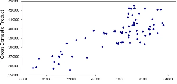
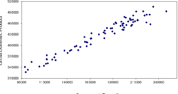
The relationship between GDP and government expenditure (GE) seems to be non-linear for some countries such as Belgium, Italy, and the United Kingdom. Scatter diagrams at Figures 1, 2, and 3 show a positive slope in the data when GDP is drawn in the horizontal axis (x) and GE in the vertical axis (y). This slope is relatively constant until a certain period of time, from which the government expenditure starts to grow faster than the GDP. Therefore, there is a change in the trend after both variables reach certain levels.
Figure 4 shows the debt-to-GDP ratio time series also for Belgium, Italy, and the UK. It can be seen that there is at least one structural break in the behavior of these variables around the year 2008 and a regime shift after this year. In this graph, a break point divides the data in high and low levels of the debt-to-GDP ratio for each country, changing the trend. These two regimes can be interpreted as good times and bad times, respectively; they are related to different GDP and GE growth rates (two separated fiscal multipliers), and they change the relationship between government expenditure and the GDP.
In the following sections, I first present a general multivariate threshold autoregressive model to explain non-lineal behaviors with two regimes. Second, I represent this model with a set of macroeconomic variables and several equations, taking into account the selection tools specified for the threshold variable. Data and results are shown for the above-mentioned three countries in Section 3. In order to improve robustness, I build a further multivariate threshold autoregressive model using a dynamic and interactive procedure in Section 4. Finally, I present some conclusions.
1
Econometric Technique and Estimation
The general multivariate threshold autoregressive model is the following:
where yj,t is the variable on the left hand side of the equation, qj,t−d are the threshold
variables, utare the errors, and zj,t are the rest of the variables on the right hand side of the
equations (including the constant).1 The coefficients are δj and θj for the regressors zj,t and
the threshold variables, respectively. Moreover, j is the number of regimes, t is the number of observations in each regime (t = T1, . . . , Tj), and d is the number of lags of the threshold
variable. Note that zj,t could include lagged values of yj,t. The non-linearity is modelled by
structural changes in the threshold variable qj,t−d thereby shifting parameters in yt and zt
for each regime. If there are strictly increasing threshold values γ1, γ2, . . . , γm (with m as the
total number of breaks), the regime j is determined by those values of qt−d (the m-partition)
in between two threshold values γj and γj+1.
The general model (1) with two regimes (j = 2) is the following:
y1,t = δ1z1,t+ θ1q1,t−d+ u1,t, if − ∞ < qt−d < γ1
y2,t = δ2z2,t+ θ2q2,t−d+ u2,t, if γ1 ≤ qt−d < ∞
(2)
where d can be 1, 2, 3, or 4.
Parameter estimation is based on the least squares principle. Following Bai and Perron (1998, 2003) and assuming the existence of only two regimes, the associated least squares estimates of the coefficients δj and θj are obtained by minimizing the sum of squared residuals
Σ2
j=1ΣTt=1[yj,t− δjzj,t− θjqj,t−d] 2
with respect to the coefficients. Given a specific threshold value γ1, the minimization of the sum square residual is a simple least squares problem.
Coefficients can be estimated by finding the threshold value and corresponding ordinary least square estimates that minimize the sum of squares across all possible sets of m = 2 threshold partitions.
Recalling (1) and (2), it is easy to see that models with two regimes will depend on values of the threshold variables qt−d regarding the threshold value γ1:
yj,t = y1,t+ y2,t = (λ) [δ1z1,t + θ1q1,t−d+ u2,t] , (3)
with λ = 1 when −∞ < qt−d < γ1 and λ = 0 when γ1 ≤ qt−d< ∞.
Auerbach and Gorodnichenko (2012) specify a model without λ. In their model, variables
1In model (1), the multivariate threshold autoregressive model is represented by only one equation for
several regimes j. For instance, yj,t is the gross domestic product. This equation corresponds to the first line
of a vector autoregressive model (VAR). Substituting each endogenous variable in model (1) as variable yj,t,
the following rows of the VAR can be obtained. For instance, the gross domestic product can be substituted by the government expenditure as the variable on left hand side of the equation. The multivariate threshold autoregressive model can be treated as a threshold vector autoregressive model (TVAR) when there are no restrictions a priori in the TVAR.
are driven by a weighted average:
xt = f (zt−1)ΠRxt−1+ (1 − f (zt−1))ΠExt−1+ ut,
where weights are given by f (zt) = [(exp(−ϕzt))/(1 + exp(−ϕzt))], and ϕ > 0. This allows
for a smooth transition and may give a better approximation of non-linearity. However, in short samples, the curvature parameter ϕ and the threshold value γ can be estimated only very imprecisely. Auerbach and Gorodnichenko (2012) overcome this problem by calibrating rather than estimating the curvature parameter using an exogenous source of information. This study uses specification (3) since λ is endogenous and depends on the threshold value γ of the threshold variable qt−d.
2
Model Representation and Selection
Recalling model (1), it can be represented by the following equation:
GDPj,t = cj+ δ1,jGEj,t+ δ2,jT Oj,t+ δ3,jP Ij,t+ δ4,jIRj,t+ θjDebtj,t−d+ uj,t (4)
where yj,t is the gross domestic product (GDP ), zj,t are the government expenditure (GE),
trade openness (T O), consumer prices (P I), and interest rate (IR), and qj,t−d is the
debt-to-GDP ratio (Debt). In equation (4), all variables have been included in differences (integrated of order 0) and augmented with lags of 1, 2, 3, and 4 periods. Therefore, time series have been transformed to I(0) to run the model with only stationary variables.
The non-linearity is captured by the threshold variable qj,t−d, which is the debt-to-GDP
ratio. This variable (Debt) divides the model in two regimes (j = 2) after a structural break is found and allows a choice between 4 lags as in model (2).
There are 4 threshold candidates for each debt-to-GDP ratio variable in each country. Therefore, the multivariate threshold autoregressive model is selected through a dynamic and interactive procedure after the time series have been transformed to I(0). Using least squares, this procedure excludes the less statistically significant variable in each interaction regarding the highest probability associated to the t statistic test of each coefficient. In order to improve the model’s robustness, all variables are included in the regression in blocks2.
Threshold variables are selected according to the Akaike selection criteria (AIC). As men-tioned before, there are four lags (d = 1, 2, 3, and 4) for each threshold variable debt-to-GDP
2The procedure can be seen as a general to specific methodology. This procedure can be used in the
multivariate threshold’s autoregressive model because, a priori, there are no restrictions in the parameters. In this model, the Akaike selection criteria (AIC) only chooses the best lag structure (delay) for the threshold variable. For further discussion on general to specific methodologies, see Campos et al. (2005)
ratio (Debt) in the multivariate threshold autoregressive model for all countries. This means that there are four candidates to determine the specification that minimizes the sum of squared residuals because the threshold variable will be lagged for 1, 2, 3, or 4 periods. AIC specifies a model asymptotically equivalent to a model that has the smallest generalized residual variance (Tsay, 1998).
3
Data and Results
There are six variables from 1996:q1 to 2015:q1 in three different countries: Belgium, Italy, and the United Kingdom. Regarding the time span, the maximum number of breaks is constrained to one. Primary sources are the World Bank, the National Bank of Belgium, the National Institute of Statistics of Italy (ISTAT), Eurostat, and the International Monetary Fund. Proxies are the following:
1) Variable GDP : The real gross domestic product at constant prices. 2) Variable GE: The government expenditure at constant prices.
3) Variable T O: The trade openness sums export of good and services plus import of goods and services in current prices divided by the real GDP .
4) Variable P I: The harmonized index of consumer prices.3
5) Variable IR: The three months reference rate of treasury certificates. 6) Variable Debt: The debt-to-GDP ratio of the central government.
The time series, such as prices in Italy, GDP in UK, and the debt-to-GDP ratio in Belgium, Italy, and UK, are integrated of order two. The rest of the variables show a one-unit root (see Table 1).
The time series have been transformed to I(0) to build a multivariate threshold autore-gressive model using the dynamic and interactive procedure. As mentioned before, this procedure excludes the less statistically significant variable in each interaction regarding the highest probability associated to the t statistic test of each coefficient. This procedure can be seen as a general to specific methodology and can be used in the multivariate threshold’s autoregressive model because, a priori, there are no restrictions in the parameters. In this model, the Akaike selection criteria (AIC) only chooses the best lag structure (delay) for the threshold variable.
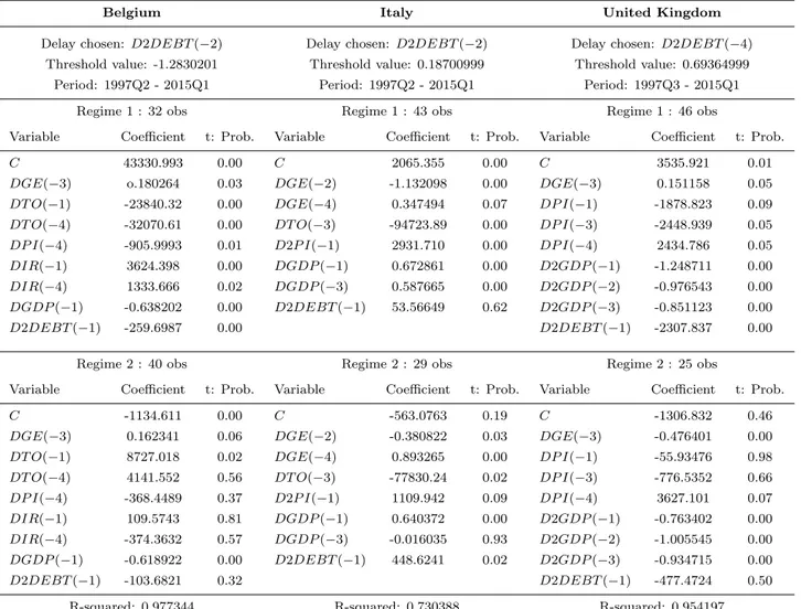
Table 2 shows results for the GDP differences in each country using the dynamic and interactive procedure described in Section 2. All variables have been transformed to I(0) to be included in the multivariate threshold autoregressive model. Coefficients have been selected
3Prices proxies are the harmonized indices of consumer prices in Italy and England. This variable is more
excluding the less statistically significant variable in each interaction regarding the highest probability associated to the t statistic test of each coefficient. As mentioned before, all variables are included in the regression in blocks in order to improve the model’s robustness. Table 2 also shows the lags chosen, threshold values for all countries, and the number of observations in both regimes. The optimal delay is selected by determining the specification model that minimizes the sum of squared residuals from all candidates in the threshold variable. There are four threshold candidates for each debt-to-GDP ratio variable. Columns 2 and 3 in each country present estimations and p-values associated to the t statistics for the representation (4) of the multivariate threshold autoregressive model (1), augmented with variables lagged at 1, 2, 3, and 4 periods. In this table, D means 1st differences, D2 is 2nd differences, C is the constant, and the negative number in parenthesis is the lag of the
variable.
The coefficients are all statistically significant at least at the 10% level in the first regime for each country, with the only exception being the value corresponding to the debt-to-GDP ratio in Italy. In Belgium, government expenditure with 3 lags is positive in the first regime and negative in the second regime. Trade openness and the GDP itself, both lagged at 1 period, are highly significant in both regimes. The debt-to-GDP ratio is only statistically significant in the first regime of this model. The threshold value is -1.28 and the R2 is equal
to 98%. In Italy, the debt-to-GDP ratio is only significant in the regime 2. Apart from the GDP lagged at 3 periods, all variables included in this model are significant in both regimes. Government expenditure is not only significant with 2 lags, but also with 4. The threshold value is 0.19 and the model explains the data well since the R2 is higher than 70%. In
the United Kingdom, government expenditure with 3 lags, prices with 4 lags, and the GDP with 1, 2, and 3 lags are significant in both regimes. The debt-to-GDP ratio is statistically significant only in the first period and the threshold value is 0.69. According to the R2, which is equal to 95%, the threshold model fits the data very well.
Variables in the right-hand side of the equation are all significant. Coefficients of the government expenditure in differences (DGE) can be only interpreted as GDP variations with respect to government expenditure variations. Therefore, regarding the sum of all significant coefficients of the DGE (lags 1, 2, 3, and 4), fiscal multipliers in the very short term are 0.2 and -0.2 in Belgium, -0.8 and 0.5 in Italy, and 0.2 and -0.5 in the United Kingdom for regimes 1 and 2, respectively. According to the set of coefficients of the government expenditure in differences, an expansionary fiscal policy seems to be counterproductive in all countries.
The two main results are the following. First, government expenditure has an impact on the GDP in both regimes in all countries. In Belgium and the United Kingdom, an expansionary government expenditure effect is positive with low values of debt-to-GDP ratio, but it is negative when the debt-to-GDP ratio increases. In Italy, this result is not conclusive.
Second, the data shows at least two regimes in a nonlinear framework if the debt-to-GDP ratio is used as a threshold variable. However, following Tsay (1998), if the debt-to-GDP ratio is included in the least squares regression, this variable has an impact on the GDP only in regime 1 in Belgium and the United Kingdom, but it does in regime 2 in Italy.
4
Conclusion
Multivariate threshold models can be invoked in order to explain fiscal multipliers considering levels of public debt. Time series related to public finance such as government debt-to-GDP ratio usually show non-linear behaviors. The inclusion of these types of variables in models which explain fiscal multipliers requires non-linear methodologies.
When explaining the behavior of real variables such as the effect of government expen-diture on output, the debt-to-GDP ratio plays an important role. The debt-to-GDP ratio (Debt) has been selected optimally as an endogenous threshold variable to evaluate non-linearities; it has been useful to identify estimators in a multivariate threshold autoregressive model (including the threshold value); and it has been a valuable tool to observe how fiscal multipliers change during good times (low levels of debt-to-GDP ratio) and bad times (high levels of debt-to-GDP ratio).
Expansionary fiscal policies seem to be counterproductive, and even negative, when other financial variables, such as levels of sovereign debt, are taken into account. Finding a rela-tionship between government expenditure, output, and public debt, this research highlights the well-known link between real and financial macroeconomic variables. Recommendations for further research include cointegration issues under non-linear models.
Acknowledgements
Financial support is acknowledged from the European Commission under the programme FP7-SSH-2013-29 and the project MACFINROBODS.
References
Auerbach, A. and Gorodnichenko, Y. (2012). Measuring the Output Responses to Fiscal Policy. American Economic Journal: Economic Policy, 4(2):1–27.
Bai, J. and Perron, P. (1998). Estimating and Testing Linear Models with Multiple Structural Changes. Econometrica, 66(1):47–78.
Bai, J. and Perron, P. (2003). Computation and analysis of multiple structural change models. Journal of Applied Econometrics, 18(1):1–22.
Blanchard, O. and Leigh, D. (2012). Are We Underestimating Short-Term Fiscal Multipliers? In World Economic Outlook of the International Monetary Fund, pages 41–43.
Blanchard, O. and Perotti, R. (2002). An Empirical Characterization of the Dynamic Effects of Changes in Government Spending and Taxes on Output. The Quarterly Journal of Economics, 117(4):1329–1368.
Campos, J., Ericsson, N., and Hendry, D. (2005). General-to-specific modeling: an overview and selected bibliography. International Finance Discussion Papers 838, Board of Governors of the Federal Reserve System (U.S.).
Christiano, L., Eichenbaum, M., and Rebelo, S. (2011). When Is the Government Spending Multiplier Large? Journal of Political Economy, 119(1):78–121.
Denes, M., Eggertsson, G., and Gilbukh, S. (2012). Deficits, Public Debt Dynamics and Tax and Spending Multipliers. The Economic Journal, pages 133–163.
Favero, C. and Giavazzi, F. (2007). Debt and the Effects of Fiscal Policy. NBER Working Papers 12822, National Bureau of Economic Research, Inc.
Ilzetzki, E., Mendoza, E., and V´egh, C. A. (2011). How Big (Small?) are Fiscal Multipliers? IMF Working Papers 11/52, International Monetary Fund.
Kim, S. and Roubini, N. (2008). Twin deficit or twin divergence? Fiscal policy, current account, and real exchange rate in the U.S. Journal of International Economics, 74(2):362– 383.
Parker, J. (2011). On Measuring the Effects of Fiscal Policy in Recessions. NBER Working Papers 17240, National Bureau of Economic Research, Inc.
Reinhart, C. M. and Rogoff, K. S. (2010). Growth in a Time of Debt. Working Paper 15639, National Bureau of Economic Research.
Tsay, R. S. (1989). Testing and Modeling Threshold Autoregressive Processes. Journal of the American Statistical Association, 84(405):231–240.
Tsay, R. S. (1998). Testing and Modeling Multivariate Threshold Models. Journal of the American Statistical Association, 93(443):1188–1202.
Vansteenkiste, I. and Nickel, C. (2008). Fiscal policies, the current account and Ricardian equivalence. Working Paper Series 935, European Central Bank.
Woodford, M. (2010). Simple Analytics of the Government Expenditure Multiplier. Working Paper 15714, National Bureau of Economic Research.
Figure 1: Belgium. Government Expenditure with respect to Gross Domestic Product (mil-lions of euros at constant prices)
Figure 2: : Italy. Government Expenditure with respect to Gross Domestic Product (millions of euros at constant prices)
Figure 3: The United Kingdom. Government Expenditure with respect to Gross Domestic Product (millions of euros at constant prices)
Table 1: Testing unit roots (augmented Dickey-Fuller) Order of integration
GDP GE TO PI IR DEBT
Belgium I(1) I(1) I(1) I(1) I(1) I(2) Italy I(1) I(1) I(1) I(2) I(1) I(2) UK I(2) I(1) I(1) I(1) I(1) I(2)
Table 2: Multivariate Threshold Model for the GDP Least Squares Regression
Belgium Italy United Kingdom
Delay chosen: D2DEBT (−2) Delay chosen: D2DEBT (−2) Delay chosen: D2DEBT (−4)
Threshold value: -1.2830201 Threshold value: 0.18700999 Threshold value: 0.69364999
Period: 1997Q2 - 2015Q1 Period: 1997Q2 - 2015Q1 Period: 1997Q3 - 2015Q1
Regime 1 : 32 obs Regime 1 : 43 obs Regime 1 : 46 obs
Variable Coefficient t: Prob. Variable Coefficient t: Prob. Variable Coefficient t: Prob.
C 43330.993 0.00 C 2065.355 0.00 C 3535.921 0.01
DGE(−3) o.180264 0.03 DGE(−2) -1.132098 0.00 DGE(−3) 0.151158 0.05
DT O(−1) -23840.32 0.00 DGE(−4) 0.347494 0.07 DP I(−1) -1878.823 0.09
DT O(−4) -32070.61 0.00 DT O(−3) -94723.89 0.00 DP I(−3) -2448.939 0.05
DP I(−4) -905.9993 0.01 D2P I(−1) 2931.710 0.00 DP I(−4) 2434.786 0.05
DIR(−1) 3624.398 0.00 DGDP (−1) 0.672861 0.00 D2GDP (−1) -1.248711 0.00
DIR(−4) 1333.666 0.02 DGDP (−3) 0.587665 0.00 D2GDP (−2) -0.976543 0.00
DGDP (−1) -0.638202 0.00 D2DEBT (−1) 53.56649 0.62 D2GDP (−3) -0.851123 0.00
D2DEBT (−1) -259.6987 0.00 D2DEBT (−1) -2307.837 0.00
Regime 2 : 40 obs Regime 2 : 29 obs Regime 2 : 25 obs
Variable Coefficient t: Prob. Variable Coefficient t: Prob. Variable Coefficient t: Prob.
C -1134.611 0.00 C -563.0763 0.19 C -1306.832 0.46
DGE(−3) 0.162341 0.06 DGE(−2) -0.380822 0.03 DGE(−3) -0.476401 0.00
DT O(−1) 8727.018 0.02 DGE(−4) 0.893265 0.00 DP I(−1) -55.93476 0.98
DT O(−4) 4141.552 0.56 DT O(−3) -77830.24 0.02 DP I(−3) -776.5352 0.66
DP I(−4) -368.4489 0.37 D2P I(−1) 1109.942 0.09 DP I(−4) 3627.101 0.07
DIR(−1) 109.5743 0.81 DGDP (−1) 0.640372 0.00 D2GDP (−1) -0.763402 0.00
DIR(−4) -374.3632 0.57 DGDP (−3) -0.016035 0.93 D2GDP (−2) -1.005545 0.00
DGDP (−1) -0.618922 0.00 D2DEBT (−1) 448.6241 0.02 D2GDP (−3) -0.934715 0.00
D2DEBT (−1) -103.6821 0.32 D2DEBT (−1) -477.4724 0.50
R-squared: 0.977344 R-squared: 0.730388 R-squared: 0.954197