AGGLOMERATION EFFECTS IN THE LABOUR MARKET: AN EMPIRICAL ANALYSIS FOR ITALY
M. De Castris, G. Pellegrini
1. INTRODUCTION1
Extensive and persistent geographic variability of the unemployment rate within the same region has been attributed to various causes: barriers to job mobility, which lower the possibility of arbitrage between local labour markets; the supply and demand of heterogeneous skills, which influence the degree of matching in the market; differences in productive structure which cause different persistent reactions in the local labour markets to sectorial shocks.
Theories identifying the “thickness” as the source of positive labour market externalities are based on improving the ability to match the skills requested by firms with those offered by workers. A recent paper by Gan and Zhang (2006) argues that geographic variability and fluctuations of the unemployment rate are caused by agglomeration externalities, linked to thick labour markets. The main idea is that clusters of firms and workers in the same area facilitate matching in local labour markets (Ciccone and Hall, 1996; Glaeser and Marc, 2001). Gan and Zhang propose a model based on heterogeneity between firms and workers with respect to their technological characteristics. It is assumed that both are located on a single-circumference circle, which represents the technological sector. The smaller the distance between workers and businesses, the higher the quality of the matching (and thus productivity and salaries) will be. It is thus possible to define the local labour market as thicker when there are more workers and businesses on this unitary circle. If the market is sufficiently dense, the expected salary from a job search is greater than the cost of the search. Workers only search for jobs under the latter condition, which is where matching occurs. Without these conditions, the level of unemployed workers grows until it reaches the minimum critical level.
This model, controlling for the effects of sectorial shocks and specific characteristics of the local labour market, envisages a negative correlation
1 We are grateful to an anonymous referee for helpful comments. We also thank Paolo Natic- chioni who offered valuable comments on earlier draft.
An earlier version of this article was presented at the XX annual conference of the Italian Association of Labour Economist.
between the average level (and maximum level) of the unemployment rate and the size of the local labour market. Some empirical tests carried out for US cities are consistent with this model.
The model cannot easily be applied to Italy for various reasons. First of all, large urban agglomerations in Italy are not the result of the development of business agglomerations, especially large ones, as has often happened in the United States. In some ways, large Italian cities are still under the impact of an urbanisation process which brought in many people from the agricultural sector, or their children, to look for a better life in urban areas where the growth of the service sector, public as well as private, offered better salaries. Tumultuous urbanisation has either broken or fragmented the information chain which matched labour supply and demand where efficient market institutions were missing. Furthermore, in some areas, especially in the South, high urban conglomeration has resulted in a deterioration of the social and civil fabric, making economic development more difficult. Actually, the sign of the effects of agglomeration on the intensity of job searching and matching results is not clear (Di Addario, 2005). Higher congestion and the unravelling of “close” social ties can increase the costs of searching and thus reduce the intensity and the results of the search. On the other hand, as Gan and Zhang (2006) stress, positive effects can come from thick markets, with a high density of workers and firms, which reduces the cost of contacts in terms of the distance between supply and demand or the cost of collecting information. Higher salaries in urban areas also increase the intensity of searches. The overall net effect will thus depend on the level of the thick market externalities as compared to the negative effects of congestion.
A second reason why the Italian situation differs from that in the United States regards the geographical location of firms. Unlike central-northern Europe and Great Britain, where firms agglomerations are found above all in urban areas, or in the United States and Canada, where they are distributed fairly evenly between urban, intermediate and rural ones, in Italy population distribution privileges intermediate zones, where areas with a high density of small and medium-sized firms, often manufacturing, are also located (OECD, 2002). Some of these areas, featuring specialised sectors called “industrial districts,” have had particularly positive results in terms of employment and growth. The lack of a clear bipolarity between urban and rural areas indicates the presence of agglomerations of firms with different characteristics, size and above all, location, from agglomerations of people.
Another way to consider this aspect concerns how to measure agglomeration from an economic point of view. The question is not settled in the literature. Actually, we can find two basic different nature of economic agglomeration: i) agglomeration across urban areas, basically measured by city size (population); ii) agglomeration across industrial clusters, measured by cluster size (employment or number of plants).
The differences in the location pattern of economic activity with respect to the urban areas can be captured by the differences in the measurement of the empirical counterpart of the two concepts. An easy way to perform a cross country comparison can be based on a simple dissimilarity index for a country k (IDk):
k i pop empi
ID =
∑
q −q (1)where qpop is population share by area i and qemp is employment share by area i in
country k.
An indicative analysis for EU regions (NUTS2) and US counties emphasizes the difference between the two areas (Table 1). As expected, the dissimilarity between the population location and the industrial location is low in United States, higher in Europe. In Italy the dissimilarity is larger than in the EU average.
TABLE 1
Dissimilarity index in USA and Europe
Countries Number of regions (a) Average population by region Average area by region (thousand square km) Dissimilarity index (all sectors) (b) Dissimilarity index (manufacturing) (c) (b/a) (c/a) USA 172 1,657,522 20,566 0.0476 0.195 0.0003 0.0011 Italy 103 562,387 2,925 0.1549 0.414 0.0015 0.0040 Germany 49 1,680,428 7,285 0.0656 0.167 0.0013 0.0034 France 96 616,592 5,666 0.0997 0.194 0.0010 0.0020 UK 133 442,390 1,833 0.0757 - 0.0006 - UE-12 110 3,103,300 20,401 0.1239 - 0.0011 -
Source: Own estimate on OECD and Eurostat data. The data are collected in the years from 1996 to 2001.
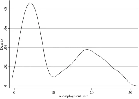
Italy is also set apart by its reduced domestic mobility as compared to other countries, such as the United States, which curbs arbitrage and accentuates regional differences. This appears clearly in macro conglomerations: if we analyse the distribution of the unemployment rate for all 784 labour systems, we can find a marked duality, which reflects territorial distribution between the Centre-North and the South (Fig.1). The reasons behind this separation of markets are well known and will not be investigated here (see, for example, Bodo and Sestito, 1991). Such a spatial dependence of data may, however, be even more extensive, involving even finer territorial levels (Pellegrini, 2002).
This analysis finds that the effect of agglomeration externalities on local labour markets, both in terms of population and industry, is not necessarily positive in Italy. In a study fairly analogous to ours, Di Addario (2005) analyses the effects of urban or industrial agglomeration on job searching in Italy. Unlike our study, the above analysis concentrates on job searching topics, utilising data regarding individuals. The conclusions appear to confirm the presence of moderately positive effects both from urbanisation (the size of the population from pre-selected areas) and industrial agglomeration on the likelihood of finding work, chiefly among the male population, but not on the intensity of the search. Some moderately positive effects of urban agglomeration on salaries have been identified even in Patacchini and Di Addario (2005). A different result is presented in de Blasio e Di Addario (2005): industrial agglomeration (i.e. italian industrial district) positively affects the likelihood of being employed.2 Moreover,
2 The literature on industrial districts shows several evidences on agglomerative externalities. See, among others, Pellegrini (2001), Becattini et al. (2003), Belussi et al. (2003).
being in an industrial district increases workers’ mobility across jobs for less-skilled individuals but reduces it for more-less-skilled ones. Therefore the authors underline that only skilled workers benefit from better quality matches.
0 .0 2 .0 4 .0 6 .0 8 De ns ity 0 10 20 30 unemployment_rate
Figure 1 – Unemployment rate distribution by the 784 local labour systems in Italy. (density function estimated by Epanechnicov Kernel)
Our paper aims to evaluate the effects of agglomeration on the local unemployment rate. The contribution of the paper is strictly empirical: we propose to disentangle urban and industrial cluster agglomeration effects, by controlling for a wide set of variables, basically related to sectorial and dimensional shocks, in order to highlight the total “size” effect in the labour market.
The study is based on a cross section analysis applied to a fine territorial grid, like that of the 784 local Italian labour systems for 2001. A simple regression between the unemployment rate and (the logarithm of) the population at the LLS level for 2001 indicates a negative (-1.2) and significant coefficient (Student’s t=5.55). The territorial variability of the unemployment rate can in fact be attributed to numerous other factors. Literature on the effects of asymmetric sectorial shocks finds that differences in sectorial structure can affect the level of unemployment rates even in the presence of nationwide sectorial shocks. Furthermore, not only the sectorial structure but also the presence of positive or negative covariance among sectors in the same area is important. If the shocks are limited to only some sectors and do not spread to the rest of the local economy, forms of compensation among sectors may take place, with a shift from a struggling to a flourishing labour
force (Neumann and Topel, 1991). Similar conclusions can be drawn about specific shocks concerning the size of firms.
Adjusting the system for the effects of sectorial and size shocks, which will be persistent due to reduced mobility, as well as those relating to geographic structure, geographical dependency and policy interventions, the results of our analysis differ from that for the United States and, to a lesser degree, for Italy. The study stresses the presence of negative and significant urbanisation externalities. The result stands up to different specifications. We obtain, instead, positive effects concerning the geographic agglomeration of firms, and their thickness, in a specific area. Furthermore, positive and significant effects can be found in local systems with features of a district. Finally, the model distinguishes the negative effects of urban agglomerations (in terms of population density) from positive firm’s agglomerations (in terms of density of local units).
The results thus show how distinct the Italian situation is. The analysis undertaken, isolating urban agglomerations from industrial ones, shows how only in the latter the positive effects of “thick” markets can overcome the negative effects caused by congestion and the weakening of informal matching facilitation mechanisms. There are numerous policy implications: first of all, if the urban agglomeration processes have negative effects on labour markets and matching quality, it is important to set up interventions to improve the availability of market information and also to reduce the cost of searches in this area. Furthermore, encouraging the creation of small and medium-sized firms agglomerations, even if not adjacent to urban areas, can improve labour market conditions and increase matching efficiency. The results show how this achievement is not necessarily linked to the presence of districts, even with all the problems of their empirical identification: from this point of view, areas which are less mono-specialised and with a greater sectorial diversification appear in our model to be more capable of absorbing negative sectorial shocks and thus reducing the average local level of unemployment.
2. THE EMPIRICAL SET-UP OF THE MODEL
Following Gan e Zhang (2006), our model considers a positive relationship between the average unemployment rate and the size of the area (LLS).
The empirical specification of the model considers the geographical dimension of data in order to estimate geographic externalities of urban and industrial agglomeration. Our starting point is a model based on a reduced form in cross-sectional context3:
i ( ) ( )
u = +α β covariatesi +ηsizei + (2) εi
3 The model of Gan and Zhang (2006) is based on a panel data, and therefore it includes also time and random effects.
where ui is the unemployment rate, i is the i-th local labour system, the covariates
are the sectorial structure and diversification, average plant size, SME share, altitude, benefits, net migration rate. As a proxy of the size of the market we use variables related to the level and to the density of population, employment, firms; as usual, in literature, we transform all size variables using a logarithmic operator. The reason is that the size is a non stationary variable but the unemployment rate is stationary (in the long run), and the logarithmic transformation gives less weight to the larger values. εi is an error term assumed iid as a first approximation. We tested
for the presence of spatial correlation in model residuals. The results clearly indicate a strong spatial correlation across area. In this case Ordinary Least Squares leads to inefficient estimators and unreliable statistical inference (Anselin, 1988). Therefore we have adopted spatial econometric methods and we estimate a model specification that considers the presence of spatial autocorrelation.
The spatial econometrics in the model is based on a spatial contiguity matrix with (nxn) elements wij representing the topology of the spatial system of the 784 local labour systems. The contiguity is defined over a 50 km. span between the LLS centroids.
The fundamental problem of this set-up is that of identifying a set of control variables able to detect geographical variability excluding the effects of size, which can subsequently be estimated with reasonable accuracy. As described above, the control variables must take into account sectorial shocks as well as the sectorial structure and risk level (in terms of sectorial covariance) of the industry, the net rate of migration, policies, such as the level of employment incentives and unemployment compensation and demographic composition.4
We tested several model specifications including different explanatory variables to examine the effect of urban and industrial agglomeration on the geographical distribution of unemployment.
The geographic, economic and social structure of Italy is vastly different from that of the United States. This requires the model to adjust to the country’s main features. First of all, the marked difference between the labour markets of the Centre-North and the South are well known. This difference cannot be detected econometrically – as shown by our analysis – but only by a dummy variable per area. Pooling the two areas leads to focus the analysis on the variability of unemployment between them: in this context the specification search tends mainly to identify variables explaining the North-South gap in unemployment. We thus preferred to undertake two separate evaluations for the two areas.5
In addition, the variability of the firm’s size is very high in Italy. In the past there were specific and persistent shocks which influenced different-sized enterprises in different ways, cutting across sectors, and which therefore must be added to the sectorial shocks.6 As a control, we have included in the model the
4 These variables are usually present in the specification adopted by Gan and Zhang. 5 We will explore the presence of territorial heterogeneity inside the two areas in the future. 6 Consider, for example, different labour market regulations between large and small firms, the different regulations concerning governance and variations in corporate law. The description of the construction of the variables of sectorial shocks and the risk level of the sectorial structure is discussed in the following chapter.
average size and number of employees of small and medium-sized firms with fewer than 200 employees. The sign of these variables will depend on the overall effects of the shock.
The unemployment rate is also affected by net migratory flows, which indicate not only tensions between the expected supply and demand of labour in different markets, but are also a measure of the localised preference (unknown) of individuals, linked to different social accessibility. Thus a variable representing net migration versus the resident population was inserted. The sign of this variability is indeterminate from the start: if the effects concerning social accessibility prevail, the result will be positive, as the population flow, under the same conditions, will increase the labour supply; if, instead, effects linked to the differences in local labour market conditions prevail, the sign will be negative (see, e.g., Elhorst 2003).
Given Italy’s geological structure, it is important to include a measurement of geographical accessibility to labour supply and demand in the model. In our case this is interpreted in terms of average altitude, to account for specific mountain LLS features. It is noteworthy that many employment incentives now exist, some major, to try to maintain a reasonable resident population in these areas to manage the environment and hydro-geological resources and preserve natural areas. The coefficient sign is thus indeterminate.
It was deemed opportune, given the number of policies with heterogeneous territorial effects, to include them in the model. A variable regarding redundancy fund programmes in the areas was inserted. This variable can also detect some specific negative LLS shocks. The sign is estimated to be positive. Variables regarding the territorial distribution of incentives were not included in the model as, given the type of incentive, they turned out to be a proxy for different levels of local distress and underdevelopment.
The size variable, identifying the thickness of the market, deserves further study. Depending on the importance given to employing specific skills in the labour market and their persistence, as well as the presence of urban or industrial agglomerations, the variable can be estimated through the population, the working-age population, the labour force and number of employees. The best specification is actually identifiable only on an empirical level, which is how we proceeded.
3. DATA AND VARIABLES
The empirical analysis of the model was carried out on the 784 local labour systems (LLS) in which Italy is divided up into. The LLS are a cluster of two or more neighbouring municipalities defined by the self-containment of daily commuter flows between home and work. Together they make up a territorial grid which covers the entire country. The concept of a local system is therefore closely connected to that of self-containment, which expresses the capability of
an area to concentrate within itself the greatest possible number of human relations existing between production areas (job sites) and those with activities linked to social life (residences) (Sforzi et al., 1997). In Italy, the practical application of this concept led to the definition of 784 LLS in 1991: 140 in the Northwest, 143 in the Northeast, 136 in the Centre and 365 in the South.
An area identified in this way is a local system: it hosts activities regarding place of residency (for example, most individual and family consumption), those connected to job sites (production and distribution expenses), and all social relations existing between these two poles. Reference to daily commutes qualifies the concept of a local system by space and time (Barbieri and Pellegrini, 2005). A local system is thus the area where supply and demand meet at a local level. It appears to us, therefore, to be the best territorial grid for the empirical analysis proposed in our study.
We have used data from Italian census on economic activities realized in 1991 and 2001; census is the main statistical source that publishes data by municipality, therefore it can be aggregated to build up the local labour system. Some statistical estimates on employment, labour force and unemployment by local labour system produced by ISTAT are also among the statistical sources of the data.7
The use of data collected over various years, despite the presence of a cross section estimate, is justified by the specification of the variables utilised to detect the effects regarding sectorial structure and diversification on unemployment for LLS. These variables are particularly important in our paper, as they allow the effects of agglomeration to be separated from those coming from sectorial risk pooling, which can also be linked to the size of the LLS.
The variable regarding the effect of sectorial structure (Indcom) considers both the nationwide industry shocks and the sectorial structure of each LLS. It is calculated by a fine sectorial detail considering 45 industries (2-digit Ateco classification for manufacturing and private services, 1-digit Ateco for pubblic services). The variable is obtained in each k-th local labour system as the sum of the products of employment share in sector i in that LLS in 1991 (qik), by the
nationwide employment growth rate in that sector in the period 1991-2001 (∆i,
that represents the national shock in sector i): 45 1 * k ik i i Indcom q = =
∑
∆ (3)7 The statistical sources are: Istat, Census of Industry and Services, years 1991 and 2001 on local units of firms and institutions by economic activity (2 digit) and by municipality; Istat, 14° General Census of Population and Residences, year 2001, by municipality; Istat, times series (estimates) 1998-2002 of domestic employees and unemployment rate by local labour system; Istat, times series 1996-2002 of employees and value added in agriculture, industry and services by local labour system; Istat, Domestic Accounts Yearbook, year 2005; Istat, Demographic Balance, year 2004 (DEMOS).
Its sign is predicted to be negative, since if the change in sectors with positive shocks is greater than that of sectors with negative shocks, there is a net positive effect on employment in the LLS.
A different effect regards the presence of sectorial diversification. Excessive productive specialisation, in fact, lowers the capacity to compensate for sectorial shocks and increases the risk of unemployment. This effect is detected in the model by a variable which represents the risk of sectorial diversification, that depends on the covariance of the labour demand across sectors. As in Neumann and Topel (1991), it was obtained using a covariance matrix Ω (size 45x45), representing the covariance of the nationwide sector-specific shocks ∆i. The covariance coefficients ωij are weighted by the employment share in i-th (qik) and j-th (qjk) sectors in the k-th
LLS in 1991:
k k k
Risk =q′Ωq (4)
In this case the predicted sign is positive, as the higher the correlation, the lower the overall effect of diversification will be.
The average size is obtained simply by dividing the number of workers by the number of local units per LLS. Variables regarding the density of employees, i.e. employees multiplied by the size in square km of the LLS, and the density of local units were used to verify the effects of industrial agglomeration.
To verify the presence of economies or diseconomies created by urban agglomerations we have considered not only demographic variables, but have also constructed two dummies: one which identifies local labour systems with an urban area of more than 300,000 inhabitants; another with populations of more than 500,000 inhabitants. Those thresholds include one of about 400,000 inhabitants, which in Patacchini and Di Addario (2005) is calculated as the optimum on the basis of the spatial self-correlation of the LLS.
The variable of territorial accessibility is identified with the average altitude of the central municipality of the LLS, the gravitational centre of the commuter flows. Another important factor influencing the unemployment rate is the migration flow. It is thus considered an indicator given the relationship between net migration flow and the resident population. This indicator is calculated for the year 2000, in order to avoid endogeneity problems.
A difference in territorial labour market policies between areas can also explain the territorial variability of unemployment. Gan and Zhang’s study on the US market considers the total amount of unemployment compensation per area. In our study, we have included in the model the number of people benefiting from a special redundancy fund (Cassa Integrazione Guadagni, from the Ministry of Labour), which was established with workers in the industrial sector in 1991, therefore avoiding potential endogeneity.
4. RESULTS
The empirical research strategy was to estimate a baseline model explaining the territorial variability of the unemployment rate in year 2001 following eq. (2) without variables regarding size. In the model we controlled for spatial autocorrelation. Then, we inserted variables explaining agglomeration in the specification and verified their statistical effects.
The baseline model was estimated using the same specification for Northern and Southern regions (Tab. 2a and 2b). The conditioning variables include the effects of sectorial structure and its diversification, size, unemployment benefits, the geographical accessibility of the area and net migratory flows. The model is proven to be statistically significant for both areas, and the variability explained is close to 25%. The signs of the variables are those predicted, especially the ones regarding risk and sectorial structure and are also the same in both areas.
Noteworthy is how in both areas a greater number of small firms lower the unemployment rate: the small and medium-sized firms turn out from this analysis to be able to adapt and absorb the labour supply of the area. This data is consistent with the empirical result of a lower unemployment rate corresponding to an increase in the average firm size. In fact, small, but not very small, firms are the ones able to export and thus flourish in domestic and international markets (see the studies in Signorini, 2000).
All the spatial tests suggest the presence of a strong spatial dependence of errors in the model8. Tests are not able to discriminate between a spatial error and a spatial lag model (Anselin et al., 1996). At the end, we presented the results for the spatial lag specification, estimated by a ML estimator. However, the results are very similar using the spatial error specification. In each estimated spatial lag model the residuals do not present spatial dependence.
Correcting for spatial dependence, the structure of the model does not change in the Centre-North; it presents only a different sign in the coefficient related to the sectorial composition variable in the South. Given the difference in the size of the economy, in the two areas it is plausible that national shocks do not capture well southern specific sectorial shocks.
The coefficient of special redundancy fund is positive: this means that the variable detects negative shocks specific for those LLS. The sign of the migratory rates in the two areas can be interpreted in terms of the effects of expectations and location preferences: migratory flows produce negative effects indicating that the areas attract new job-hunting workers (though this increase in the labour supply does not correspond to the same demand).
The specification of urban agglomerations was calculated through different variables. The main results are the following:
TABLE 2a Baseline model Estimation method: OLS(*)
Variables Centre-North South
Sectorial diversification 2.91
(0.009) (0.003) 11.81
Sectorial composition -14.58
(0.000) (0.312) -10.50
Average plant size (0.000) -1.32 (0.000) -3.32
SME share -7.08 (0.000) (0.048) -8.26 Altitude -0.22 (0.000) (0.000) -0.61 Unemployment benefits 25.96 (0.008) (0.020) 27.28
Net migration rate -9.76
(0.611) -130.18 (0.033)
R2 0.23 0.24
Adjusted R2 0.22 0.22
Root M.S.E. 1.61 4.54
Moran’s I (0.053) 1.93 (0.016) 2.41
Spatial error (LM test) 581.18 (0.000) (0.000) 1234.6
Spatial lag (LM test) (0.000) 28.55 (0.000) 247.4
n. obs. 419 365
(*) p-value between parentheses.
TABLE 2b
Baseline model corrected for spatial dependence. Estimation method: ML (*)
Variables Centre-North South
Sectorial diversification 3.97
(0.000) (0.065) 5.41
Sectorial composition -10.19
(0.001) (0.657) 3.42
Average plant size (0.000) -1.37 (0.000) -2.51
SME share -8.16 (0.000) (0.047) -6.14 Altitude -0.27 (0.000) (0.000) -0.89 Unemployment benefits 21.39 (0.022) (0.232) 10.39
Net migration rate -28.18
(0.126) (0.041) -92.33
ρ(spatial lag coefficient) 0.023
(0.000) (0.000) 0.017 log likelihood -772.21 -960.80 Variance ratio 0.293 0.571 Squared corr. 0.294 0.571 Wald test of ρ =0 (0.000) 38.25 285.084 (0.000) LR test of ρ =0 (0.000) 36.59 210.677 (0.000) LM test of ρ =0 (0.000) 28.56 247.402 (0.000) n. obs. 419 365
1. the agglomerative effect due to the size of the population and the labour forces is positive and significant in both areas (Tab. 3 for the Centre-North and Tab. 4 for the South). Even if the working-age population is utilised, the sign does not change.
2. the results are no different if one tries to isolate the effect caused by large urban agglomerations. The impact of big cities is always positive and significant in the Centre-North (Tab. 3) and in the South (Tab. 4).
3. the effect due to a higher density of the population per square km, which thus regards the relative “thickness” of markets, is positive but not significant in both areas (Tab. 3 and 4).
TABLE 3
Urban agglomeration in the Centre-North of Italy Estimation method: ML (*)
Centre-North Variables
Mod.2 Mod.3 Mod.4 Mod.5 Mod.6 Mod.7 Sectorial diversification 6.32
(0.000) (0.000) 4.30 (0.000) 4.25 (0.000) 4.45 (0.000) 6.21 (0.000) 6.32 Sectorial composition -21.28
(0.000) (0.000) -11.89 (0.000) -11.81 (0.000) -12.64 (0.000) -20.98 (0.000) -21.28 Average plant size -1.88
(0.000) (0.000) -1.38 (0.000) -1.37 (0.000) -1.48 (0.000) -1.89 (0.000) -1.88 SME share -5.46 (0.000) (0.000) -7.70 (0.000) -7.57 (0.000) -7.94 (0.000) -5.77 (0.000) -5.46 Altitude -0.14 (0.002) (0.000) -0.26 (0.000) -0.26 (0.000) -0.24 (0.002) -0.15 (0.002) -0.14 Unemployment benefits 13.36 (0.131) (0.020) 21.57 (0.019) 21.69 (0.024) 20.82 (0.117) 13.96 (0.131) 13.36 Net migration rate -48.69
(0.006) (0.216) -22.82 (0.244) -21.47 (0.140) -26.97 (0.006) -48.30 (0.006) -48.69 Ln(population) 0.70 (0.000) - - - Urban areas > 300.000 inhabitant - 1.60 (0.016) - - - - Urban areas > 500.000 inhabitant - - 2.20 (0.006) - - - Population density - - - 9.84E-04 (0.007) - - Ln(labour force) - - - - 0.66 (0.000) - Ln(population 15-64) - - - 0.70 (0.000)
ρ(spatial lag coefficient) 0.020 (0.000) 0.023 (0.000) 0.023 (0.000) 0.023 (0.000) 0.021 (0.000) 0.021 (0.000) log likelihood -747.31 -769.32 -768.51 -768.57 -749.91 -746.93 Variance ratio 0.373 0.303 0.306 0.306 0.365 0.374 Squared corr. 0.373 0.303 0.306 0.306 0.365 0.374 Wald test of ρ =0 (0.000) 29.78 (0.000) 36.78 (0.000) 35.84 (0.000) 34.02 (0.000) 31.75 (0.000) 30.68 LR test of ρ =0 (0.000) 28.77 (0.000) 35.25 (0.000) 34.39 (0.000) 32.71 (0.000) 30.61 (0.000) 29.62 LM test of ρ =0 (0.000) 23.52 (0.000) 27.60 (0.000) 26.72 (0.000) 25.15 (0.000) 24.98 (0.000) 24.22 n. obs. 419 419 419 419 419 419
TABLE 4
Urban agglomeration in the South of Italy Estimation method: ML (*)
South Variables
Mod.2 Mod.3 Mod.4 Mod.5 Mod.6 Mod.7 Sectorial diversification 6.35
(0.030) (0.060) 5.52 (0.055) 5.61 (0.000) 5.39 (0.030) 6.35 (0.028) 6.42 Sectorial composition 1.35
(0.861) (0.710) 2.87 (0.726) 2.70 (0.651) 3.49 (0.876) 1.20 (0.887) 1.09 Average plant size -2.71
(0.000) (0.000) -2.53 (0.000) -2.53 (0.000) -2.48 (0.000) -2.74 (0.000) -2.74 SME share -2.77 (0.408) (0.069) -5.66 (0.087) -5.33 (0.041) -6.35 (0.446) -2.55 (0.486) -2.33 Altitude -0.78 (0.000) (0.000) -0.87 (0.000) -0.87 (0.000) -0.92 (0.002) -0.77 (0.000) -0.77 Unemployment benefits 8.48 (0.327) (0.231) 10.40 (0.194) 11.28 (0.227) 10.51 (0.335) 8.34 (0.347) 8.12 Net migration rate -96.59
(0.031) (0.059) -85.97 (0.069) -82.66 (0.039) -93.59 (0.028) -98.67 (0.028) -98.42 Ln(population) 0.57 (0.013) - - - Urban areas > 300.000 inhabitant - (0.247) 2.05 - - - - Urban areas > 500.000 inhabitant - - (0.081) 4.29 - - - Population density - - - -3.43E-04 (0.595) - - Ln(labour force) - - - - (0.009) 0.61 - Ln(population 15-64) - - - (0.005) 0.63
ρ(spatial lag coefficient) 0.017
(0.000) (0.000) 0.017 (0.000) 0.017 (0.000) 0.017 (0.000) 0.017 (0.000) 0.017 log likelihood -957.76 -960.13 -959.28 -960.65 -957.40 -956.93 Variance ratio 0.578 0.573 0.575 0.572 0.579 0.580 Squared corr. 0.578 0.573 0.575 0.572 0.579 0.580 Wald test of ρ =0 (0.000) 291.09 (0.000) 286.13 (0.000) 284.68 274.26 (0.000) (0.000) 292.69 (0.000) 293.14 LR test of ρ =0 (0.000) 214.03 (0.000) 211.26 (0.000) 210.45 204.55 (0.000) (0.000) 214.93 (0.000) 215.17 LM test of ρ =0 (0.000) 251.72 (0.000) 247.83 (0.000) 245.83 234.04 (0.000) (0.000) 253.06 (0.000) 253.23 n. obs. 365 365 365 365 365 365
(*) p-value between parentheses.
Overall, the positive relationship between demographic size of the LLS and unemployment level shows that the negative effects of urban agglomerations, in relation to the presence of congestion, breakdowns in information and informal trust chains and the greater difficulty in job searching, prevail over the positive ones of a greater “thickness” of the market. It is to be noted that this does not appear to be attributable to a possible weakness of the specification adopted for the basic model: the coefficients are similar and do not change their sign even when variables regarding the size of the labour market are inserted.
The analysis thus tried to evaluate the effects which can be attributed to industry agglomeration, utilising different variables here as well. The results are partially different from those obtained for urban agglomerations:
1. the use of variables such as number of employees and their logarithm leads to a positive (but not significant) coefficient in both areas; the coefficients of employment density are negative (and not significant). Such variables are,
however, closely correlated of those regarding population, and thus detect only very approximately the effects of industrial agglomerations (Tab. 5 and 6). 2. the results regarding the number of plants and their density are very different.
The coefficient is negative and significant in the Centre-North (as expected where there are thick market externalities) but also in the South.
3. if, instead, we simultaneously insert population density and plants density for both areas, we obtain a positive coefficient for the former and a negative one for the latter. They are significant in both cases. This could mean that when the effects of urban agglomeration are negative we observe positive firms’ agglomerations. The result can be interpreted by claiming that while the first variable detects congestion diseconomies, the second one detects thick market economies.
TABLE 5
Industrial agglomeration in the Centre-North of Italy Estimation method: ML (*)
Centre-North Variables
Mod.8 Mod.9 Mod.10 Mod.11 Mod.12 Mod.13 Sectorial diversification 3.82
(0.000) (0.002) 3.55 (0.000) 4.32 (0.000) 5.88 (0.000) 4.28 (0.000) 4.14 Sectorial composition -10.63
(0.001) (0.054) -6.37 (0.000) -12.00 (0.000) -19.55 (0.000) -11.80 (0.001) -10.62 Average plant size -1.29
(0.000) - (0.000) -1.46 (0.000) -1.94 (0.000) -1.44 (0.000) -1.42 SME share -7.52 (0.000) - (0.000) -8.08 (0.000) -6.75 (0.000) -8.10 (0.000) -8.29 Altitude -0.27 (0.000) (0.000) -0.268 (0.000) -0.25 (0.000) -0.18 (0.000) -0.25 (0.000) -0.26 Unemployment benefits 20.88 (0.025) (0.004) 27.65 (0.000) 21.25 (0.000) 15.41 (0.000) 21.21 (0.021) 21.44 Net migration rate -26.86
(0.146) (0.058) -37.59 (0.144) -26.86 (0.000) -43.56 (0.000) -27.94 (0.126) -28.14 Industrial district -0.21 (0.329) -1.07 (0.000)) - - - - Employee density - - 1.51E-03 (0.071) - - - Ln(employee) - - - 0.52 (0.000) - - Plants density - - - - 6.35E-03 (0.084) - Ln(plants) - - - - 0.02 (0.326)
ρ(spatial lag coefficient) 0.024 (0.000) 0.023 (0.000) 0.023 (0.000) 0.022 (0.000) 0.023 (0.000) 0.023 (0.000) log likelihood -771.73 -802.61 -770.58 -758.89 -770.72 -771.72 Variance ratio 0.295 0.183 0.299 0.337 0.298 0.295 Squared corr. 0.295 0.183 0.299 0.337 0.298 0.295 Wald test of ρ =0 38.85 (0.000) 32.16 (0.000) 35.38 (0.000) (0.000) 32.57 (0.000) 35.28 (0.000) 37.10 LR test of ρ =0 (0.000) 37.15 (0.000) 30.98 (0.000) 33.96 (0.000) 31.37 (0.000) 33.87 (0.000) 35.55 LM test of ρ =0 (0.000) 29.08 (0.000) 21.33 (0.000) 26.21 (0.000) 25.25 (0.000) 26.11 (0.000) 27.64 n. obs. 419 419 419 419 419 419
TABLE 6
Industrial agglomeration in the South of Italy Estimation method: ML (*)
South Variables
Mod.8 Mod.9 Mod.10 Mod.11 Mod.12 Mod.13 Sectorial diversification 3.71
(0.212) (0.009) 7.07 (0.072) 5.27 (0.049) 5.82 (0.068) 5.34 (0.045) 5.92 Sectorial composition 1.25
(0.870) (0.683) 3.18 (0.624) 3.79 (0.758) 2.39 (0.636) 3.65 (0.780) 2.17 Average plant size -2.32
(0.000) - -2.43 (0.000) (0.000) -2.69 (0.000) -2.43 (0.000) -2.63 SME share -4.68 (0.132) - -6.44 (0.038) (0.139) -4.92 (0.038) -6.41 (0.168) -4.60 Altitude -0.87 (0.000) (0.000) -0.82 (0.000) -0.94 (0.000) -0.85 (0.000) -0.95 (0.000) -0.84 Unemployment benefits 8.72 (0.313) (0.565) 4.94 (0.228) 10.48 (0.278) 9.47 10.47 (0.23) (0.284) 9.34 Net migration rate -80.83
(0.073) (0.000) -182.0 (0.038) -93.97 (0.039) -93.59 (0.041) -92.11 (0.030) -98.69 Industrial district -2.57 (0.009) (0.000) -3.58 - - - - Employee density - - -2.62E-03 (0.375) - - - Ln(employee) - - - (0.330) 0.23 - - Plants density - - - - (0.266) - -0.012 Ln(plants) - - - (0.224) 0.28
ρ(spatial lag coefficient) 0.017
(0.000) (0.000) 0.018 (0.000) 0.017 (0.000) 0.017 (0.000) 0.017 (0.000) 0.017 log likelihood -957.38 -974.02 -960.40 -960.32 -960.18 -959.46 Variance ratio 0.579 0.539 0.572 0.572 0.573 0.574 Squared corr. 0.579 0.539 0.572 0.572 0.573 0.574 Wald test of ρ =0 (0.000) 293.15 (0.000) 296.51 (0.000) 278.79 286.56 (0.000) (0.000) 281.71 (0.000) 284.05 LR test of ρ =0 (0.000) 215.18 (0.000) 217.03 (0.000) 207.13 211.50 (0.000) (0.000) 208.78 (0.000) 210.09 LM test of ρ =0 (0.000) 252.99 (0.000) 253.49 (0.000) 238.18 248.45 (0.000) (0.000) 240.41 (0.000) 240.64 n. obs. 365 365 365 365 365 365
(*) p-value between parentheses.
4. a test was performed by isolating the most densely industrialised LLS. In this case the “district” classification of LLS appearing in Istat (1997) was used. Obviously, if the controls regarding the number of small firms and average size are maintained, the district dummy is negative but not very significant. By removing such controls, the variable is always negative and very significant, indicating the presence of agglomeration externalities (Tab. 7 and 8).
The results regarding plants agglomerations, even if somewhat conflicting, seem to indicate the presence of agglomeration economies with positive effects on the labour market.
TABLE 7
Urban and industrial agglomeration in the Centre-North of Italy Estimation method: ML (*)
Centre-North Variables
Mod.14 Mod.15 Mod.16 Mod.17 Sectorial diversification 4.95
(0.000) (0.000) 5.20 (0.000) 4.14 (0.000) 4.43 Sectorial composition -12.25
(0.000) (0.000) -12.25 (0.001) -10.80 (0.000) -15.27
Average plant size -0.48
(0.023) (0.000) -1.67 (0.000) -1.29 (0.000) -1.36 SME share -1.81 (0.141) (0.140) -1.84 (0.000) -7.43 (0.000) -6.54 Altitude -0.15 (0.001) (0.001) -0.15 (0.000) -0.21 (0.000) -0.23 Unemployment benefits 14.48 (0.076) (0.097) 13.65 (0.039) 18.84 (0.037) 19.13
Net migration rate -45.01
(0.005) (0.005) -46.03 (0.080) -31.56 (0.175) -24.53 Ln(population) 4.17 (0.000) (0.000) - 4.09 - Ln(employee) -3.55 (0.000) - - - Ln(plants) - (0.000) - -3.49 - Population density - - 6.51E-03 (0.000) 3.24E-03 (0.000) Employee density - - (0.000) - -0.01 Plants density - - - (0.001) -0.16
ρ(spatial lag coefficient) 0.017
(0.000) (0.000) 0.017 (0.000) 0.022 (0.000) 0.022 log likelihood -713.44 -716.98 -762.04 -763.554 Variance ratio 0.466 0.457 0.327 0.322 Squared corr. 0.466 0.457 0.327 0.322 Wald test of ρ =0 (0.000) 26.22 (0.000) 27.37 (0.000) 33.73 (0.000) 31.80 LR test of ρ =0 (0.000) 25.43 (0.000) 26.51 (0.000) 32.44 (0.000) 30.65 LM test of ρ =0 (0.000) 20.88 (0.000) 21.83 (0.000) 24.90 (0.000) 23.41 n. obs. 419 419 419 419
(*) p-value between parentheses.
5. CONCLUSIONS
The model proposed by Gan and Zhang (2006) shows how the presence of agglomeration externalities, linked to the presence of thick labour markets, can explain the geographic variability of the unemployment rate (and its fluctuations). The authors, in any case, do not explain if agglomeration depends on urbanisation, i.e. aggregations of people, or else depends on the presence of industrial clusters, i.e. firm’s aggregations. This is because in the United States the two agglomerations tend to coincide, as large cities often grow alongside their industrial areas.
This does not occur in many European countries, including Italy. In Italy, especially, many firms clusters (in some cases referred to as districts) spring up in areas adjacent to medium sized or small cities. The transposition of the results of the model is thus not automatic, and requires an adaptation of the spatial distribution of the population and firms.
TABLE 8
Urban and industrial agglomeration in the South of Italy Estimation method: ML (*)
South Variables
Mod.14 Mod.15 Mod.16 Mod.17 Sectorial diversification 4.95
(0.000) (0.000) 5.16 (0.000) 4.77 (0.077) 5.15 Sectorial composition 7.70
(0.000) (0.000) 7.24 (0.001) 5.01 (0.593) 4.10
Average plant size 0.40
(0.023) (0.000) -2.09 (0.000) -2.30 (0.000) -2.3 SME share -0.41 (0.141) (0.140) -0.63 (0.000) -6.14 (0.095) -5.24 Altitude -0.87 (0.001) (0.001) -0.86 (0.000) -0.92 (0.000) -0.94 Unemployment benefits 13.46 (0.076) (0.097) 11.33 (0.253) 9.93 (0.276) 9.42
Net migration rate 27.94
(0.005) (0.005) 4.11 (0.080) -91.28 (0.104) -74.51 Ln(population) 6.76 (0.000) (0.000) 7.03 - Ln(employee) -6.37 (0.000) - - Ln(plants) - (0.000) -6.77 Population density - - 2.95E-03 (0.223) 4.43E-03 (0.054) Employee density - - -1.56E-02 (0.158) Plants density - - (0.030) -0.08
ρ(spatial lag coefficient) 0.015
(0.000) (0.000) 0.015 (0.000) 0.017 (0.000) 0.017 log likelihood -936.94 -939.72 -959.66 -958.33 Variance ratio 0.624 0.618 0.574 0.577 Squared corr. 0.624 0.618 0. 574 0. 577 Wald test of ρ =0 (0.000) 233.65 228.39 (0.000) (0.000) 274.35 272.03 (0.000) LR test of ρ =0 (0.000) 180.60 177.37 (0.000) (0.000) 204.60 203.28 (0.000) LM test of ρ =0 (0.000) 204.41 198.55 (0.000) (0.000) 233.41 231.58 (0.000) n. obs. 365 365 365 365
(*) p-value between parentheses.
By utilising a fine territorial grid provided by the 784 LLS, and taking into account the structural differences between the regions of the Centre-North and those of the South, in our study the unemployment rate (as a measurement of the efficiency of the labour market) was compared to variables representing urban and industrial agglomerations, conditioning the relationship in the face of sector, size, geographical and policy effects.
The results clearly show that, unlike what was empirically found by Gan and Zhang (2006) for the United States and by Di Addario (2005), even if only to a slight degree, for Italy, urban agglomerations have negative effects on the unemployment rate of the area. This is true not only for large and very large cities: this negative correlation is maintained at different levels. The same results show, even if less clearly, how industrial agglomerations have positive effects on the labour market, confirming and extending the results of de Blasio e Di Addario (2005). The results are more interesting when we consider both agglomerations: the
industrial clusters have a positive effect on the employment, while is still negative the effect of urban agglomeration. We can conclude that only an aggregation of firms empirically generates the market externalities often mentioned by the model.
This conclusion is not surprising: in Marshall’s studies as well, labour market pooling was indicated as a source of industrial district externalities. The conclusion that such effects only occur among firms is less automatic. This can mean that an aggregation of firms is able to already take into account the presence of specific skills in the area, which in turn strengthen their competitive potential. An urban aggregation, instead, follows a different logic which does not necessarily link the requested skills to firms.
There are many policy implications that can be derived from our results. First of all, government should increase the circulation of labour market information in order to enhance the matching between job seekers and labour positions even in urban areas. Incentive for reducing the costs of search cannot obviously be limited to the case of contiguity between the supply and demand of skills, but also regards the acquisition of information and knowledge which often occurs through informal chains, less strong in urban centres. Improvements in the quality of the matching require policies able to disseminate information which can substitute those channels. It is important to reduce the costs of getting information in order to avoid the discouraging effect on job search activities.
The study also suggests how supporting the creation of small and medium-sized business clusters, even if not in the vicinity of urban areas, can improve labour market conditions and increase matching efficiency. The result is not necessarily linked to the presence of industrial districts: from this point of view, less specialised areas with a larger sectorial diversification turn out to be, from our model, more capable of absorbing negative sectorial shocks and of reducing the average level of unemployment in the area. The aforementioned policies, in any case, must take care not to constrain the districts and reduce their dynamism, which is its main source of innovation and competitiveness (Pellegrini, 2001).
Department of Public Institutions, Economy and Society MARUSCA DE CASTRIS
University of Rome “Roma Tre”
Department of Economic Theory and GUIDO PELLEGRINI
Quantitative Methods for Political Choice Sapienza, University of Rome
REFERENCES
L. ANSELIN (1988), Spatial econometrics: methods and models, Kluwer, Dordrecht.
L. ANSELIN, A. BERA, R. FLORAX AND M. YOON(1996),Simplediagnostic tests for spatialdependence,
“Regional Science and Urban Economics”, 26, 1, pp. 77-104.
G. BARBIERI, G. PELLEGRINI(2005), I Sistemi locali del lavoro: uno strumento per la politica economica
in Italia e in Europa, in G. Esposito (ed.), “Scritti in onore di Antonino Giannone”,
ISCONA, Roma.
G. BECATTINI, M. BELLANDI, G. DEI OTTATI, F. SFORZI (2003), From industrial districts to local
F. BELUSSI, G. GOTTARDI, E. RULLANI (eds.) (2003), The technological evolution of industrial districts,
Kluwer, Boston.
G. BODO, P. SESTITO(1991),Le vie dello sviluppo, Il Mulino, Bologna.
A. CICCONE, R. HALL(1996),Productivity and the density of economic activity,“American Economic
Review”,86,1, pp. 54-70.
G. DE BLASIO, S. DI ADDARIO(2005),Do workers benefit from industrial agglomeration?, “Journal of
Regional Science”, 45, 4, pp. 797-827.
S. DI ADDARIO, E. PATACCHINI(2005),Wages and the city: the Italian case, University of Oxford,
Department of Economics, Working Paper Series, ref. 243.
S. DI ADDARIO(2005),Job search in thick markets: evidence from Italy, Oxford Department of
Economics, Discussion Papers Series, n. 235.
J. P. ELHORST(2003), The mystery of regional unemployment differentials: theoretical and empirica
explanations,“Journal of Economic Surveys”,17, 5, pp. 709-748.
L. GAN, Q. ZHAN(2006),The thick market effect on local unemployment rate fluctuations,“Journal of
Econometrics”, 133, pp. 127-152.
E. GLAESER, D. MARC(2001),Cities and skill,“Journal of Labour Economics”,19,2, pp.
316-342.
ISTAT(1997), I sistemi locali del lavoro 1991,Roma, Istat. A. MARSHALL(1890), The Principles of Economics,London.
G. NEUMANN, R. TOPEL (1991), Employment risk, diversification and unemployment, “Quarterly
Journal of Economics”, 106, 4, pp. 1341-1365.
OECD(2002),Territorial database, source and methodology, OECD, Paris.
E. PATACCHINI, S. DI ADDARIO(2005),Agglomerazione urbana e salari in Italia, in L. BRUCCHI (eds),
Temi di economia del lavoro, Il Mulino, Bologna.
G. PELLEGRINI(2001), La struttura produttiva delle piccole e medie imprese italiane: il modello dei
distretti, “Banca, Impresa e Società”, n. 2.
G. PELLEGRINI(2002),Proximity, polarization and local labour market performance,“Network and
Spatial Economics”, 22, pp. 151-174.
S.S. ROSENTHAL, W. STRANGE (2001), The determinants of agglomeration, “Journal of Urban
Economics”, 50, pp. 91-229.
L.F. SIGNORINI (ed.) (2000),Lo sviluppo locale. Un’indagine della Banca d’Italia sui distretti indu-
striali,Roma, Donzelli.
F. SFORZI, C. WYMER, A. A. GILLARD(1997),I sistemi locali del lavoro nel 1991,in Istat, I sistemi
locali del lavoro 1991, Argomenti n.10, Istat, Roma.
SUMMARY
Agglomeration effects in the labour market: an empirical analysis for Italy
Extensive and persistent geographic variability of the unemployment rate within the same region has been attributed to various causes. Some theories identify the “thickness” of markets as the source of positive externalities affecting labour market by improving the ability to match the skills requested by firms with those offered by workers. A recent paper by Gan and Zhang (2006) empirically confirms this hypothesis for the US labour markets. Agglomeration can be defined as aggregation of people, basically measured by city size, or as aggregation of firms, measured by cluster size (employment or number of plants). However, the population location and the industrial location are by far more similar in United States than in Europe and in Italy. Our paper aims to evaluate the effects of agglomeration on the local unemployment rate. The new methodological
contribution of the study is the identification of both urban and industrial cluster agglomeration effects, using a wide set of control variables. Adjusting the system for the effects of sectorial and size shocks, as well as those relating to geographic structure and policy interventions, the results of our analysis differ from that for the United States. The study stresses the presence of negative and significant urbanisation externalities. We obtain, instead, positive effects concerning the geographic agglomeration of firms, and their thickness, in a specific area. Furthermore, positive and significant effects can be found in local systems with features of a district. Finally, the model distinguishes the negative effects of urban agglomerations (in terms of population density) from positive firm’s agglomerations (in terms of density of local units).