DOUBLE LOMAX DISTRIBUTION AND ITS APPLICATIONS
Punathumparambath Bindu1
Department of statistics, Govt. Arts & Science College, Kozhikode, Kerala, India Kulathinal Sangita
Department of Mathematics and Statistics,University of Helsinki, Finland.
1. Introduction
Laplace distributions are tractable lifetime models in many areas, including life testing and telecommunications. The properties of the Laplace distribution and applications, were given by Johnson, Kotz and Balakrishnan (1990), Kotz et al. (2001). In the present study we deal with the ratio of two independent and iden-tically distributed Laplace distribution. The ratio of two random variables X and Y arises in many statistical studies and have applications in various areas such as economics, nuclear physics, meteorology and genetics. The distribution of
X/Y has been studied by several authors in particular when X and Y are
inde-pendent random variables from the same family, see Marsaglia (1965), Korhonen and Narula (1989) for normal family, Press (1969) for student’s t family, Provost (1989) for gamma family, Pharm-Gia (2000) for beta family and so on. Nadaraja and Kotz (2006) considered X and Y respectively normal and Laplace random variables distributed independent of each other.
The present study introduces a new family of distributions called double Lo-max distribution. The double LoLo-max distribution is the ratio of two independent and identically distributed classical Laplace distributions. Also the double Lomax distribution can be obtained by compounding classical Laplace distribution with exponential density (Gamma density with shape parameter α = 1 and scale pa-rameter β = 1). The compound distribution is of interest for the study of produc-tion/inventory problems, since it provides a flexible description of the stochastic properties of the system. These distributions play a central role in insurance and other areas of applied probability modelling such as queuing theory, reliability etc. The Laplace model is an alternative to the normal model in situations where the normality assumption do not hold. In a similar way the double Lomax distribution is an alternative to the Cauchy distribution. This family is a special case of type II compound Laplace distribution (Kotz et al., 2001; Bindu et al., 2012).
The double Lomax distribution is a natural symmetric extension of Lomax distribution to the real line. A random variable X is said to have a Lomax distri-bution, Lomax (α, β) with parameters α and β if its probability density function (pdf) is
f (x; α, β) = αβα(β + x)−(α+1), x > 0, α, β > 0. (1) The Lomax distribution is widely known as the type II Pareto distribution, and is related to the 4-parameter type II generalized beta distribution and the 3-parameter Singh-Maddala distribution, as well as the beta distribution of the second kind.
This article is organized as follows. In section 2, the double Lomax distribution is derived, and various properties explored. In section 3 we describe the maximum likelihood estimation of parameters using the BFGS algorithm of optim function (Nash J. C., 1990) in R (R Core Team, 2015). The application of the double Lomax distribution is illustrated in section 4 and we conclude in section 5.
2. Double Lomax distribution
The double Lomax distribution is the ratio of two independent and identically distributed classical Laplace distributions and defined as follows.
Definition 1. Let X1 and X2 be two independent and identically distributed
(i.i.d.) standard classical Laplace random variables. Then the corresponding prob-ability distribution of X = X1/X2 is given by
f (x) = 1
2 (1 +|x|)2, −∞ < x < ∞. (2) The Laplace distribution can also be expressed as the difference of two i.i.d exponentials and hence, Xi
d
= IiWi, for i = 1, 2 where, Wi∼ Exp(1), for i = 1, 2
and Ii′s are independent of Wi and takes values±1 with equal probabilities.
Then the cdf can be given by
F (x) = 1 2(1−x), for y≤ 0 ( 1−2(1+x)1 ) , for y > 0. (3)
Remark 2. Let X1 and X2 be two independent and identically distributed
(i.i.d.) standard classical Laplace random variables. Then the corresponding prob-ability distribution of Z =|X1/X2| is given by
f (z) = 1
(1 + z)2, 0 < z <∞, (4)
which is the pdf of the Lomax distribution. Hence the random variable X having pdf given by Eq. (2) may be referred to as the double Lomax distribution (DLD).
The double Lomax distribution, which is the extension of the Lomax distribution over the real line is defined as follows.
Definition 3. A random variable X is said to have a double Lomax
distribu-tion with parameters µ and σ, DLD(µ, σ) if its probability distribudistribu-tion funcdistribu-tion is, FX(x) = 1 2(1+(µ−x)σ ), x≤ µ 1− 1 2(1+(x−µ)σ ), x > µ, (5)
and the probability density function is, fX(x) = 1 2 σ ( 1 +|(x−µ)σ | )2,−∞ < x < ∞. (6) If X ∼ DLD(0, 1) then it is referred as the standard double Lomax
distribu-tion. The corresponding probability distribution and density functions are given
by Eq. (2) and Eq. (3), respectively.
If X has the standard double Lomax distribution and q = F (x), then x =
F−1(q) and quantiles ξq can be written explicitly as follow
ξq = ( 1−2q1 ) , for 0 < q≤ 12 ( 1 2(1−q)− 1 ) , for 12 ≤ q < 1. (7)
Thus if X has the double Lomax distribution with cdf given by Eq. (5) then quantiles ´ξq is obtained as ´ξq = µ + σξq. In particular, the first and the third
quartiles are given by
Q1= ´ξ1/4= µ− σ, Q2= ´ξ1/2= µ, Q3= ´ξ3/4= µ + σ.
Hence, µ and σ can be estimated using corresponding sample quantities so that an estimator of µ, ˆµ = ˆQ2, and an estimator of σ, ˆσ = Qˆ3− ˆQ1
2 , the sample quartile deviation.
Proposition 4. Let P1, P2, P3 and P4 be i.i.d. Pareto Type I random
vari-ables with density 1/x2, x≥ 1. Then X
1= log(P1/P2) and X2= log(P3/P4) are
i.i.d. standard classical Laplace random variable (Kotz et al., 2001) and hence X = X1/X2 has the standard double Lomax density.
Proposition 5. Let P1, P2, P3 and P4 be i.i.d. standard power function
distribution with parameter p, having the density
f (x) = pxp−1, p > 0, x∈ (0, 1).
Then the random variables X1= p log(P1/P2) and X2 = p log(P3/P4) are i.i.d.
standard classical Laplace (Kotz et al., 2001) and hence X = X1/X2 has the
2.1. Properties
The following properties of the probability density function Eq. (2) hold. For most of them the proof is immediate.
• The standard double Lomax distribution is symmetric around the location
parameter µ = 0.
• Like the Cauchy distribution, the standard double Lomax distribution has
infinite mean and variance. But for this distribution the fractional moments
E|X|α exit for 0 < α < 1 and more robust estimates for location parameter and variance, such as median and Median Absolute Deviation (MAD) exist.
• The αthmoment of X, E(Xα) exist for 0 < α < 1 and is given as follows.
E(Xα) = Γ(1 + α)Γ(1− α).
• If X is distributed as the standard double Lomax then 1/X also has the
standard double Lomax distribution. That is, the standard double Lomax distribution is log symmetric. Also,
X+ d= 1/X+,
where X+follows the half standard double Lomax distribution, or the Lomax distribution, and
X− d= 1/X−,
where X− has the standard double Lomax density truncated below zero.
• The standard double Lomax distribution is heavy tailed than Laplace
distri-bution and has more area concentrated towards the center (mode). Note that the tail probability of double Lomax density is ¯F ∼ cx−α, α = 1 as x→ ± ∞, where ¯F is the survival function. The heavy tail characteristic makes this
density appropriate for modelling network delays, signals and noise, finan-cial risk or microarray gene expression or interference which are impulsive in nature.
• The standard Double Lomax distribution is unimodal mode x = 0 since the
distribution is monotonically increasing and convex on (−∞, 0) and mono-tonically decreasing and concave on (0,∞).
• The standard double Lomax distribution is a scale-mixture of the Laplace
distribution. Note that every symmetric density on (−∞, ∞) which is com-pletely monotone on (0,∞) is a scale mixture of Laplace distribution (Dreier, 1999).
• The half standard double Lomax density (Lomax density)is a scale-mixture
of exponential densities. Note that every completely monotone density on (0,∞) is a scale mixture of exponential densities on (0, ∞) (Steutel, 1970).
−8 −6 −4 −2 0 1 2 3 4 5 6 7 8 0.0 0.2 0.4 0.6 0.8
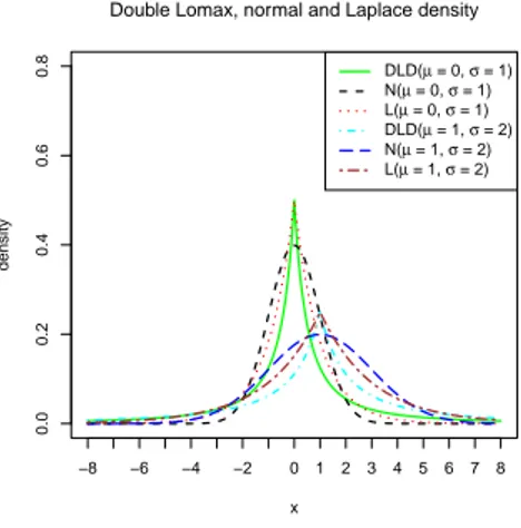
Double Lomax, normal and Laplace density
x density DLD(µ = 0, σ = 1) N(µ = 0, σ = 1) L(µ = 0, σ = 1) DLD(µ = 1, σ = 2) N(µ = 1, σ = 2) L(µ = 1, σ = 2)
Figure 1 – Double Lomax density functions for various values of parameters.
• If X ∼ DLD(µ, σ), then Y = aX +b ∼ DLD(b+aµ, aσ) where a ∈ R, b ∈ R
and a ̸= 0. Hence, the distribution of a linear combination of a random variable with DLD(µ, σ) distribution is also DLD. If X ∼ DLD(µ, σ), then
Y = (X− µ)/σ ∼ DLD(0, 1), which can be called as the standard double
Lomax distribution.
Proposition 6. Let f be a symmetric (about zero) probability density on (−∞, ∞)
which is completely monotone on (0,∞) (Kotz et al., 2001). Then there exists a distribution G on (0,∞) such that
f (x) = ∫ ∞ 0 1 2ye −y|x| dG(y); x̸= 0,
while the characteristic function corresponding to f is
Ψ(t) = ∫ ∞
0 1
1 + t2/y2dG(y), − ∞ < t < ∞.
Remark 7. The converse of the proposition Eq. (6) holds well. Thus every
density f (x) of the form given above with some cdf G on (0,∞) is a symmetric density on (−∞, ∞) which is completely monotone on (0, ∞) (Kotz et al., 2001).
The shape of the density Eq. (6) is given in Figure 1 along with the normal and Laplace density functions. From Figure 1 we can see that for double Lomax density (DLD) more area is concentrated towards the center and has heavier tails than normal and Laplace distribution.
3. Likelihood and estimation
In this section we study the problem of estimating unknown parameters, Θ = (µ, σ), of the double distribution. To estimate the parameter µ we use the quantile estimation. The quantile estimate of µ is the ˆµ = sample median.
Let X = (X1,· · · , Xn) be independent and identically distributed samples from
a double Lomax distribution with parameters Θ. The log-likelihood function takes the form
logL(µ, σ; X) =−nlog2 − nlogσ − 2
n
∑
i=1
log (1 +|(xi− µ)/σ|) .
The MLE of σ for given µ = ˆµ is obtained the following score equation.
ˆ σ = 2 n n ∑ i=1 |xi− ˆµ| [ 1 + |xi−ˆµ| ˆ σ ].
Maximum likelihood estimates (MLE) of the parameter σ can be obtained by solving the score equation. Numerical methods are needed to solve this score equation. In our illustration, the maximization of the likelihood is implemented using the BFGS algorithm of optim function (Nash J. C., 1990) in R (R Core Team, 2015). Estimates of the standard errors were obtained by inverting the numerically differentiated information matrix at the maximum likelihood estimates.
3.1. Simulation
In this section we use the simulation study of the double Lomax distribution to validate the estimation algorithm developed in R. Since we can express the distribution function of the double Lomax distribution as well as its inverse in closed form, the inversion method of simulation is straightforward to implement. We performed simulation studies for various choices of parameters to evaluate the performance of the estimation procedure. We generated 1000 samples, each of size n = 1000 from the double Lomax distribution with parameters (µ, σ) by inverting the distribution function Eq. (5) in R and then applied the algorithm to obtain the MLEs of the parameters. The results from the 1000 replications are presented in Table 1. It is clear from Table 1 that the estimation algorithm works satisfactorily for various choices of parameters and the asymptotic standard errors of the maximum likelihood estimators agree well with the sample standard deviations over the replications.
4. Application
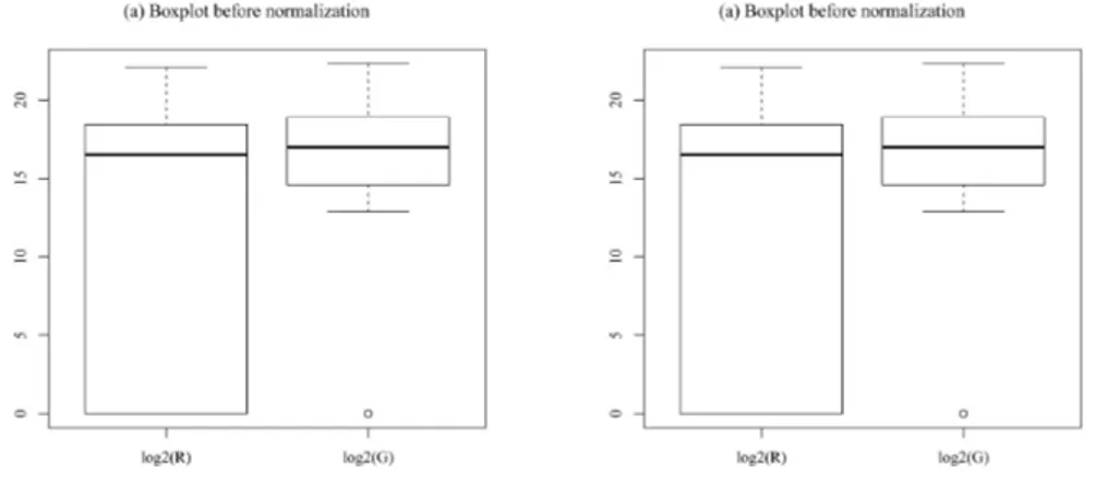
In this section we apply the double Lomax distribution to model the distribution of a cDNA dual dye microarray gene expression data set. The dataset consists of self-self hybridizations of 19 different cell lines, as well as the Stratagene uni-versal reference RNA (Yang et al., 2002). The self-self arrays were normalized using (Lowess) locally weighted linear regression method (Cleveland and Delvin, 1988)(Cleveland and Delvin, 1988). This method is capable of removing intensity dependence in log2(Ri/Gi) values and it has been successfully applied to
microar-ray data (Yang et al., 2002), where Ri is the red dye intensity and Gi is the green
dye intensity for the ith gene. For example, see Figure 2 for the box plots of
TABLE 1
Simulation study - Maximum likelihood estimates of (µ, σ) for various choices of parameters. Standard deviations over 1000 replications of dataset of size n = 1000. SE
stands for the asymptotical standard errors of the maximum likelihood estimates.
µ σ µˆ ˆσ SD(ˆµ) SE(ˆµ) SD(ˆσ) SE(ˆσ) -0.05 0.5 -0.049 0.508 0.002 0.001 0.010 0.009 1 - 0.051 0.978 0.001 0.002 0.051 0.070 1.5 - 0.051 1.464 0.003 0.001 0.025 0.093 -0.01 0.5 - 0.011 0.461 0.003 0.001 0.021 0.028 1 -0.009 1.154 0.002 0.002 0.104 0.046 1.5 -0.009 1.548 0.002 0.003 0.112 0.067 0.01 0.5 0.009 0.515 0.001 0.005 0.022 0.041 1 0.011 1.052 0.002 0.002 0.041 0.065 1.5 0.011 1.451 0.002 0.002 0.072 0.089 0.05 0.5 0.049 0.527 0.001 0.003 0.036 0.046 1 0.049 1.029 0.001 0.002 0.053 0.099 1.5 0.051 1.544 0.002 0.003 0.086 0.121 TABLE 2
Application - maximum likelihood estimates and their asymptotical standard deviations for DLD, Laplace and normal.
DLD Laplace Normal
ˆ
µ -0.025 (0.009) -0.025 (0.003) 0.011 (0.002) ˆ
σ 0.066 (0.003) 0.327 (0.002) 0.283 (0.001)
each distribution of the gene expression has a similar shape and exhibits heavier tails compared to a Gaussian distribution. We fitted the double Lomax distribu-tion, Laplace and normal to the normalized microarray intensities. The maximum likelihood estimates of the parameters and standard errors (SE) are reported in Table 2.
Figure 3 depicts a histogram of the gene expression data, the fitted DLD, Laplace and normal density functions evaluated at the MLEs. Heavy-tailed dis-tributions are proper distribution to accommodate outliers in the data; in case of microarray gene expression the number of genes differently expressed is usually a very small proportion of the whole dataset. Hence we believe that statistical model presented in this paper will be very useful in estimation and detection problems involving gene expression data.
We used Akaike’s Information Criterion (AIC) (Akaike, 1973; Burnham and Anderson, 1998) and Bayesian Information Criterion (BIC) (Schwarz, 1978) to assess the appropriateness of DLD over the Laplace and normal. The AIC and
BIC are given by
AIC =−2logL + 2K and BIC = −2logL + K log(n),
where logL = log(Lf(ˆθ|x1,· · · , xn)) is the log-likelihood of the data x1,· · · , xn
es-Figure 2 – Box plots of intensities from microarray Experiment N T 2 3 (a) Before
nor-malization, (b) After loess normalization.
Figure 3 – Fitted double Lomax probability density function (red line), Laplace density
function (blue dash) and normal density function (green dot) to the microarray gene expression data.
timated, ˆθ is the maximum likelihood estimate of the parameters of f and n is
the sample size. Note that AIC does not explicitly take into account the sample size as BIC does. However, in most cases AIC and BIC are of similar nature and give consistent results for model selection. Here AIC and BIC values coin-cide. A smaller value of AIC or BIC indicates a better fit. We calculated AIC and BIC for the DLD(µ, σ), L(µ, σ) and N (µ, σ) distributions for the dataset examined. AICDLD − AICL = −1216 < 0, AICDLD − AICN = −2364 < 0,
BICDLD− BICL = −1216 < 0 and BICDLD− BICN = −2364 < 0. Hence
DLD(µ, σ) distribution had a lower AIC, and BIC for the dataset compared to
Laplace and normal. A smaller value of AIC and BIC indicates a better fit, and hence, DLD seems to fit the data better than Laplace and normal.
5. Conclusion
The standard double Lomax random variable is the ratio of two i.i.d. classical Laplace variables. The standard double Lomax distribution (DLD) is a flexible distribution that can take heavy tails into account. These are some of the common features of the data related to financial modelling and microarray modelling. The standard double Lomax distribution is log symmetric and heavy tailed like Cauchy distribution. Hence the double Lomax distribution (DLD) introduced in this pa-per is useful in analysing datasets that are symmetric, leptokurtic, and deviate considerably from the classical symmetric distributions such as normal, Laplace, logistic etc. among others.
We illustrated the application of DLD to a microarray gene expression data set of Yang et al. (2002). From Figure 3, it is clear that the tail behaviour and peakdness of the data is captured better in DLD than in normal. The reduction in AIC or BIC for DLD compared to Laplace and normal is small for the dataset considered in the earlier section. As our distribution is a heavy-tailed, it is a proper distribution to accommodate outliers in the data. In case of microarray gene expression data, the number of genes differently expressed is usually a very small proportion of the entire collection of genes studied. Hence, the probability distribution presented in this paper will be very useful in estimation and detection problems involving gene expression data.
The ratio of two i.i.d. classical Laplace variables is log symmetric and heavy tailed like Cauchy distribution. The Laplace model is an alternative to the normal model in situations where the normality assumption do not hold. In a similar way the ratio of independent and identically distributed Laplace distribution is an alternative to the Cauchy distribution. Hence this distribution can be useful in analyzing data sets which exhibits heavy tail. The heavy tail characteristic makes this density appropriate for modeling network delays, signals and noise, financial risk or interference which are impulsive in nature.
Laplace distributions and its generalizations have recently got more importance in various fields including financial modeling, image processing, communication en-gineering, modeling currency exchange rate, interest rates, stock price changes etc. Hsu (1979) used Laplace distribution to model the position errors observed in large navigation systems. DLD could be applied to modeling error distribution in cases
where the distribution deviates from normal. The DLD introduced in this paper can be useful in analyzing data sets which exhibits heavy tails and peakedness. We found that DLD is suitable for modeling microarray gene expression data, since it is having thick tails and sharp peak in the middle. Another application is in modeling of the size distribution of diamonds from a large mining area. Our model also found applications in many fields including modeling of the shapes of long bright gamma-ray bursts discussed by Norris et al. (1996); behavioural systems; random fluctuations of response data.
Acknowledgements
The first author is grateful to the Department of Science & Technology, Govern-ment of India, New Delhi, for financial support under the Women Scientist Scheme (WOS-A (2008)), Project No: SR/WOS-A/MS-09/2008.
References
H. Akaike (1973). Information theory and an extension of the maximum
likeli-hood principle. In Kotz and Johnson (eds.), Breakthroughs in Statistics, Vol
I. Springer Verlag, New York, pp. 610–624.
P. P. Bindu, K. Sangita, G. Sebastian (2012). Asymmetric type II
com-pound Laplace distribution and its application to microarray gene expression.
Computational Statistics and Data analysis, 56, pp. 1396–1404.
K. Burnham, D. Anderson (1998). Model selection and Inference, Springer, New York.
W. S. Cleveland, S. J. Delvin (1988). Locally weighted regression: an
ap-proach to regression analysis by local fitting. Journal of American Statistical
Association, 83(403), pp. 596–610.
I. Dreier (1999). Inequalities for real characteristic functions and their moments. Ph.D. Dissertation, Technical University of Dresden, Germany.
C. Fernandez, M. F. J. Steel (1998). On Bayesian modelling of fat tails and
skewness. Journal of American Statistical Association, 93, pp. 359–371.
D. A. Hsu (1979). Long-tailed distributions for position errors in navigation, Applied Statistics, 28, pp. 62–72.
Johnson, Kotz, Balakrishnan (1990). Distributions in Statistics. Volume I: Continous univariate distributions, Boston, Houghton Miffin.
P. J. Korhonen, S. C. Narula (1989). The probability distribution of the ratio
of the absolute values of two normal variables. Journal of Statistics Computation
S. Kotz, T. J. Kozubowski, K. Podgorski (2001). The Laplace Distribution
and Generalizations: A Revisit with Applications to Communications. Eco-nomics, Engineering and Finance. Birkh¨auser, Boston.
G. Marsaglia (1965). Ratios of normal variables and ratios of sums of uniform
variables. Journal of American Statistical Association, 60, pp. 193–204.
Nadaraja, Kotz (2006). A note on the ratio of normal and Laplace random
variables. S M A, 15, pp. 151–158.
J. C. Nash (1990). Compact Numerical Methods for Computers. Linear Algebra
and Function Minimisation. Adam Hilger.
J. P. Norris, R. J. Nemiroff, J. T. Bonnell, J. D. Scargle, C. Kouve-liotou, W. S. Paciesas, C. A. Meegan, G. J. Fishman (1996). Attributes
of pulses in long bright gamma-ray bursts, Astrophysical Journal, 459, pp. 393–
412.
T. Pharm-Gia (2000). Distributions of the ratios of independent beta variables
and applications. Communications in Statistics Theory and Methods, 29, pp.
2693–2715.
S. J. Press (1969). The t ratio distribution. Journal of American Statistical Association, 64, pp. 242–252.
S. B. Provost (1989). On the distribution of the ratio of powers of gamma
random variables. Pakistan Journal of Statistics, 5, pp. 157–174.
R Core Team (2015). R: A language and environment for statistical
com-puting. R Foundation for Statistical Computing, Vienna, Austria. http: //www.R-project.org/.
G. Schwarz (1978). Estimating the dimension of a model. Annals of Statistics, 6, pp. 461–464.
F. W. Steutel (1970). Preservation of Infinite Divisibility Under Mixing and
Related Topics. Mathematisch Centrum, Amsterdam.
Yang, Yee Hwa, Dudoit, Sandrine, Luu, Percy, Lin, M. David, Peng, Vivian, Ngai, John, Speed, P. Terence (2002). Normalization for cDNA
microarray data: a robust composite method addressing single and multiple slide systematic variation. Nucl. Acids Res., 30(4), e15.
Summary
The Laplace distribution and its generalizations found applications in a variety of dis-ciplines that range from image and speech recognition (input distributions) and ocean engineering to finance. In the present paper, our major goal is to study the family of distribution called the double Lomax distribution which is the ratio of two independent
and identically distributed classical Laplace distributions. Also the double Lomax distri-bution can be obtained by compounding classical Laplace distridistri-bution with exponential density. The important statistical properties of double Lomax distribution are explored. Also the relationships with other families of distributions are established. Maximum likelihood estimation procedure is employed to estimate the parameters of the proposed distribution and an algorithm in R package is developed to carry out the estimation. A simulation study is conducted to validate the algorithm. Finally, the application of our model is illustrated. We have used a microarray data set for illustration.
Keywords: Double Lomax distribution; Laplace distribution; Lomax distribution;