Analysis of Perturbed Fractals for Antenna Synthesis

UNIVERSITY

OF TRENTO

DIPARTIMENTO DI INGEGNERIA E SCIENZA DELL’INFORMAZIONE 38123 Povo – Trento (Italy), Via Sommarive 14

http://www.disi.unitn.it

ANALYSIS OF PERTURBED FRACTALS FOR ANTENNA SYNTHESIS

L. Lizzi and A. Massa

January 2011

Analysis of Perturbed Fractals for Antenna Synthesis      L. Lizzi* and A. Massa  ELEDIA Group ‐ Department of Information Engineering and Computer Science  University of Trento, Via Sommarive 14, I‐38050 Trento, Italy  E‐mail: leonardo.lizzi@disi.unitn.it, Web‐page: http://www.eledia.ing.unitn.it      Introduction   

In  the  last  years  there  has  been  an  increasing  demand  for  compact  and  multi‐ service  systems  driven  by  the  great  expansion  of  telecommunications  sectors  such  as  mobile  telephony  or  personal  communications.  The  development  of  these  systems  involves  the  synthesis  of  innovative  antennas  characterized  by  small  dimensions  and  able  to  manage  simultaneously  different  communication  standards  [1].  In  this  framework,  fractal‐shaped  antennas  are  promising  solutions  thanks  to  their  properties.  Among  them,  the  self‐similarity  property  and the possibility to shrink an infinite‐length curve in a finite area make fractal  geometries  excellent  candidates  for  both  multi‐band  [2][3]  and  miniaturization  [4] purposes. However, standard fractal‐shaped antennas, as the Koch monopole  [5],  usually  present  an  harmonic  behavior  rather  than  a  real  multi‐band  behavior. Possible solutions to such a limitation are based on the perturbation of  the fractal shape [6][7]  in order to increase the degrees of freedom during the  synthesis  process  for  better  tuning  and  controlling  the  working  frequencies  of  the arising structure. 

In this paper, the effects of some variations of the geometry of a Koch‐like fractal  antenna are carefully analyzed to define some a‐priori rules for the synthesis of  efficient  antennas.  Towards  this  end,  a  set  of  descriptive  parameters  which  “control”  the  antenna  structure  is  defined  and  the  achievable  antenna  performances  are  studied  by  means  of  numerical  simulations  to  define  some  analytic  relationships  for  the  behavior  of  resonant  frequencies.  However,  since  only  an  exhaustive  search  of  the  whole  set  of  possible  combinations  of  the  antenna  parameters  would  provide  an  analytic  synthesis  tool,  the  analysis  is  devoted  to  provide  a  suitable  initialization  for  global  optimization  procedures  aimed  at  finding  the  best  set  of  antenna  parameters  without  excessive  computational costs.    Fractal Antenna Analysis and Synthesis    Let us consider the Koch‐like geometry derived from the Koch curve described in  [8]. Following the notation in [8], the antenna is generated from the Koch curve  by iteratively (let   be the fractal iteration index) applying the Hutchinson  k

    Fig. 1 – Koch‐like antenna geometry at k =1.    operator. At the  ‐th stage the antenna structure is uniquely determined by the  descriptive vector    k k w   ( ) ( )

{

}

where    is  the  length  of  the  ‐th  antenna  segment  at  the  ‐th  iteration,  whereas   is the  ( )k i l i k ( )k j θ j‐th angle at the same stage. As an example, the normalized  (with respect to the antenna length L) antenna geometry at k =1 is shown in  Fig. 1. For the sake of simplicity, let us focus on the Koch geometry at the first  iteration to study the impact of the geometrical perturbations on the  resonant  frequency behavior of the fractal antenna. More specifically, the location of the  first  M  resonant frequencies  f_m( )1;m=1,...,M is analyzed. Towards this purpose,  the  following  constraints  are  imposed  on  the  antenna  structure:  , 

,  and  ( ) ( )1 2 1 3 l l = ( ) ( )1 1 1 2 θ θ = ( ) ( ) ( )

( )

l = − − .  The  last  requirement  forces  the  antenna  to  always  occupy  the  same  area.  Moreover,  in  order  to  avoid  any  reliance  on  the  working  frequency,  the  resonant  frequencies  have  been  normalized  such  that  ( )

( ) ( ) ( ) m M f f f f _std m std m m m ; 1,..., ~ 1 1 = − = ,  where   

denote  the  first 

( ) _{m M}

f_mstd ; =1,...,

M resonant  frequencies  of  the  standard  Koch‐like  monopole  antenna ( ( ) ( ) 3 1 1 2 1 1 = l = l and  ( ) 3 1 1 π θ = ).   

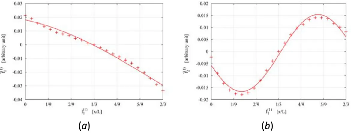
To  illustrate  some  representative  results  from  the  analysis,  two  different  test  cases are reported in the following. The first one is aimed at verifying the effects  of varying   while keeping the others set to the reference monopolar structure  ( ( )1 1 l ( ) 3 1 1 2 = l   and  ( ) 3 1 1 π

θ = ).  Figure  2  shows  the  first  and  the  second  resonant  frequencies  in  correspondence  with  the  admissible  values  of  ( )1

1

l .  A  sinusoidal  behavior, characterized by the following relations 

(a)  (b)   

Fig. 2 –Behavior of (a) ~f₁( )1 and (b) ~f₂( )1  varying the l₁( )1  parameter.      (a)  (b)    Fig. 3 – Behavior of (a)  1( )1 ~ f and (b)  2( )1 ~ f  varying the l2( )1  parameter.    ( )

(

)

(

)

is  obtained  whatever  the  resonant  frequency.  In  the  second  test  case,    is  varied in the range  ( )1 2 l ⎥⎦ ⎤ ⎢⎣ ⎡ 3 2 , 0  while  ( ) 3 1 1 1 = l  and  ( ) 3 1 1 π θ = . As it can be noticed (Fig.  3), the resonant frequencies vary with a linear trend according to the following    ( ) ( ) ( ) ( )1 2 1 2 1 2 1 1 742 . 0 276 . 0 ~ 646 . 0 231 . 0 ~ l f l f − = − =   (3)   

From  an  engineering  perspective,  (2)  and  (3),  as  well  as  the  others  obtained  varying  the  other  descriptors,  give  a  set  of  an  a‐priori  information  to  be  fully  exploited  as  a  suitable  initialization  for  a  successive  optimization  process  for 

refining the choice of the best solution (i.e., the optimal antenna parameters). As  a  matter  of  fact,  a  good  initialization  usually  results  in  an  efficient  method  for  minimizing the computational time as well as the required resources. 

Conclusions   

In  this  paper,  the  effects  of  geometrical  perturbations  on  the  geometry  of  a  reference  fractal  antenna  have  been  carefully  analyzed  to  provide  a  set  of  analytic rules for describing the resonant behavior of the antenna. As regards to  the antenna synthesis, the obtained results can be profitably used to initialize an  optimization  process  for  identifying  an  optimal  solution  thus  allowing  non‐ negligible saving of the computational resources. 

References   

[1] C.  Puente,  J.  Romeu,  and  A.  Cardama,  “Fractal‐shaped  antennas”  in 

Frontiers  in  Electromagnetics,  D.  H.  Werner,  R.  Mittra,  Eds.  Piscataway, 

NJ: IEEE Press, 2000, pp. 48‐93. 

[2] C.  Puente,  J.  Romeu,  R.  Pous,  and  A.  Cardama,  “On  the  behavior  of  the  Sierpinski multiband antenna,” IEEE Trans. Antennas Propag., vol. 46, pp.  517‐524, Apr. 1998. 

[3] R. K. Mishra, R. Ghatak, and D. R. Poddar, “Design formula for Sierpinski  gasket  pre‐fractal  planar‐monopole  antennas,”  IEEE  Antennas  Propag. 

Mag., vol. 50, no. 3, pp. 104‐107, Jun. 2008. 

[4] J. P. Gianvittorio and Y. Rahmat‐Samii, “Fractal antennas: a novel antenna  miniaturization  technique,  and  applications,”  IEEE  Antennas  Propag. 

Mag., vol. 44, no. 1, pp. 20‐36, Feb. 2002. 

[5] C.  P.  Baliarda,  J.  Romeu,  and  A.  Cardama,  “The  Koch  monopole:  a  small  fractal antenna,” IEEE Trans. Antennas Propag., vol. 48, no. 11, pp. 1773‐ 1781, Nov. 2000. 

[6] C.  Puente,  J.  Romeu,  R.  Bartolome,  and  R.  Pous,  “Perturbation  of  the  Sierpinski  antenna  to  allocate  operating  bands,”  Electron.  Lett.,  vol.  32,  pp. 2186‐2188, Nov. 1996. 

[7] R. Azaro, F. De Natale, M. Donelli, E. Zeni, and A. Massa, “Synthesis of a  prefractal  dual‐band  monopolar  antenna  for  GPS  applications,”  IEEE 

Antennas Wireless Propag. Lett., vol. 5, pp. 361‐364, 2006. 

[8] D.  H.  Werner,  P.  L.  Werner,  and  K.  H.  Church,  “Genetically  engineered  multiband  fractal  antennas,”  Electron.  Lett.,  vol.  37,  no.  19,  pp.  1150‐ 1151, Sept. 2001.