A Full Year Evaluation of the CALIOPE-EU Air
Quality Modeling System over Europe for 2004
M. T. Paya, M. Piota, O. Jorbaa, S. Gass´oa,b, M. Gonc¸alvesa,b, S. Basarta, D.
Dabdubd, P. Jim´enez-Guerreroc, J. M. Baldasanoa,b,∗
aEarth Sciences Department. Barcelona Supercomputing Center. Barcelona, Spain bEnvironmental Modelling Laboratory, Technical University of Catalonia, Barcelona, Spain
cNow at: Department of Physics, University of Murcia, Murcia, Spain
dDepartment of Mechanical and Aerospace Engineering, University of California, Irvine.
California, USA
Abstract
The CALIOPE-EU high-resolution air quality modeling system, namely WRF-ARW/HERMES-EMEP/CMAQ/BSC-DREAM8b, is developed and applied to Eu-rope (12 km × 12 km, 1hr). The model performances are tested in terms of air quality levels and dynamics reproducibility on a yearly basis. The present work describes a quantitative evaluation of gas phase species (O3, NO2 and SO2) and
particulate matter (PM2.5 and PM10) against ground-based measurements from the EMEP (European Monitoring and Evaluation Programme) network for the year 2004. The evaluation is based on statistics. Simulated O3 achieves
satisfac-tory performances for both daily mean and daily maximum concentrations, espe-cially in summer, with annual mean correlations of 0.66 and 0.69, respectively. Mean normalized errors are comprised within the recommendations proposed by the United States Environmental Protection Agency (US-EPA). The general trends and daily variations of primary pollutants (NO2 and SO2) are satisfactory. Daily
mean concentrations of NO2correlate well with observations (annual correlation
r=0.67) but tend to be underestimated. For SO2, mean concentrations are well
simulated (mean bias=0.5 µg m−3
) with relatively high annual mean correlation (r=0.60), although peaks are generally overestimated. The dynamics of PM2.5 PM2.5 and PM10 is well reproduced (0.49 < r < 0.62), but mean concentrations
∗Corresponding author. Tel.: +34 93 413 77 19; fax: +34 93 413 77 21 Email address:[email protected](J. M. Baldasano)
remain systematically underestimated. Deficiencies in particulate matter source characterization are discussed. Also, the spatially distributed statistics and the general patterns for each pollutant over Europe are examined. The model perfor-mances are compared with other European studies. While O3statistics generally
remain lower than those obtained by the other considered studies, statistics for
NO2, SO2, PM2.5 and PM10 present higher scores than most models.
Keywords: Air quality, Model evaluation, Europe, High resolution, Ozone, Particulate matter
1. Introduction
1
Atmospheric pollutants have significant impact on many main fields. One
2
of the major areas impacted is human health. High correlations between
long-3
term exposure to fine particles and human health issues have been detected in
4
population-based studies for several decades (Lave and Seskin, 1970; Thibodeau
5
et al., 1980; Lipfert, 1994; P´enard-Morand et al., 2005). The latest studies even
6
quantify the effects of aerosols on human lifespan. It is suggested that a decrease
7
of 10 µg m−3 in the concentration of fine particles may lead to an increase in
8
life expectancy of 0.61 years (Pope et al., 2009). Another major area impacted
9
by atmospheric pollutants is climate change. Particles scatter and absorb solar
10
and infrared radiation in the atmosphere. In addition, they alter the formation and
11
precipitation efficiency of liquid-water, ice and mixed-phase clouds (Ramanathan
12
et al., 2001). Radiative forcing associated with these perturbations affects climate
13
(Chylek and Wong, 1995; Jacobson, 2001). A third area impacted by air quality
14
pollutants is atmospheric visibility. Since the size of atmospheric aerosols is
sim-15
ilar to the wavelength of visible light, light is scattered and absorbed as it travels
16
through the atmosphere (Japar et al., 1986; Adams et al., 1990). In brief,
atmo-17
spheric pollutants are part of a highly complex system that affects the physics,
18
chemistry, and life on the planet.
19
The European Commission (EC) and the US-EPA, among others, have shown
20
great interest in the transport and dynamics of pollutants in the atmosphere.
Ac-21
cording to the European directives (European Commission, 1996, 2008), air
qual-22
ity modeling is a useful tool to understand the dynamics of air pollutants, to
an-23
alyze and forecast the air quality, and to develop plans reducing emissions and
24
alert the population when health-related issues occur. Both have set ambient air
25
quality standards for acceptable levels of O3(European Commission, 2002), NO2 26
and SO2 (European Commission, 1999, 2001), PM2.5 and PM10 in ambient air 27
(European Commission, 1999, 2001, 2008).
28
The CALIOPE project, funded by the Spanish Ministry of the Environment
29
and Rural and Marine Affairs (Ministerio de Medio Ambiente y Medio Rural
30
y Marino), has the main objective to establish an air quality forecasting system
31
for Spain (Baldasano et al., 2008b). In this framework, a high-resolution air
32
quality forecasting system, namely
WRF-ARW/HERMES-EMEP/CMAQ/BSC-33
DREAM8b, has been developed and applied to Europe (12 km × 12 km, 1hr) as
34
well as to Spain (4 km × 4 km, 1hr). The simulation of such a high-resolution
35
model system has been made possible by its implementation on the MareNostrum
36
supercomputer hosted by the Barcelona Supercomputing Center-Centro Nacional
37
de Supercomputaci´on (BSC-CNS). In order to reduce uncertainties, the model
38
system is evaluated with observational data to assess its capability of reproducing
39
air quality levels and the related dynamics.
40
A partnership of four Spanish research institutes composes the CALIOPE
41
project: the BSC-CNS, the “Centro de Investigaciones Energ´eticas,
Medioambi-42
entales y Tecnol´ogicas” (CIEMAT), the Institute of Earth Sciences Jaume Almera
43
of the “Centro Superior de Investigaciones Cient´ıficas” (IJA-CSIC) and the
“Cen-44
tro de Estudios Ambientales del Mediterraneo” (CEAM). This consortium deals
45
with both operational and scientific aspects related to air quality monitoring and
46
forecasting. BSC-CNS and CIEMAT lead the model developments of the project
47
while IJA-CSIC and CEAM are in charge of retrieving observational data for
eval-48
uation processes. Current experimental forecasts are available through
49
http://www.bsc.es/caliope.
50
Several operational air quality forecasting systems already exist in Europe
51
(see http://gems.ecmwf.int or http://www.chemicalweather.eu, Hewitt and Griggs,
52
2004; COST, 2009). CALIOPE advances our understanding of atmospheric
dy-53
namics in Europe as follows. First, CALIOPE includes a high-resolution
compu-54
tational grid. Most models use a horizontal cell resolution of at least 25 km ×
55
25 km for domains covering continental Europe. CALIOPE uses a 12 km x 12
56
km cell resolution to simulate the European domain. Second, CALIOPE includes
57
a complex description of the processes involved in the modeling of particulate
58
matter. Both are important factors to obtain accurate results of air pollutant
con-59
centrations in a complex region such as southern Europe (Jim´enez et al., 2006).
60
Moreover, to date, none of the existing European operational systems include the
61
influence of Saharan dust on a non-climatic basis. Dust peaks cannot be
repre-62
sented by introducing boundary conditions derived from dust climatological data
63
due to the highly episodic nature of the events in the region (1- to 4-day average
64
duration) (Jim´enez-Guerrero et al., 2008). When considering only anthropogenic
emissions, chemical transport model simulations underestimate the PM10
con-66
centrations by 30-50%, using the current knowledge about aerosol physics and
67
chemistry (Vautard et al., 2005a).
68
The purpose of the present paper is to provide a quantitative assessment of
69
the capabilities of the WRF-ARW/HERMES-EMEP/CMAQ/BSC-DREAM8b air
70
quality modeling system to simulate background concentrations of gas and
par-71
ticulate phase in the European domain. In the rest of the paper, this model
sys-72
tem will be named “CALIOPE-EU”. This evaluation intends to warrant the use
73
of such simulation for further nested calculations on the smaller domain of the
74
Iberian Peninsula (principal goal of the CALIOPE project). The results are
eval-75
uated statistically and dynamically, compared to performance goals and criteria,
76
and to other model performances.
77
In this paper, Sect. 2 describes the models, the observational dataset and the
78
statistical parameters calculated. Section 3 analyses the model results against
79
available measurement data for the year 2004 and the modeled annual
distribu-80
tion of O3, NO2, SO2, PM2.5 and PM10. A thorough comparison with other 81
European studies is presented in Sect. 4. Conclusions are drawn in Sect. 5.
82
2. Methods
83
2.1. Model Description
84
CALIOPE is a state-of-the-art modeling framework currently under further
de-85
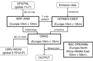
velopment. As shown in Fig. 1, CALIOPE-EU is a complex system that integrates
86
a meteorological model (WRF-ARW), an emission processing model
(HERMES-87
EMEP), a mineral dust dynamic model (BSC-DREAM8b), and a chemical
trans-88
port model (CMAQ) together in an air quality model system.
89
2.1.1. Meteorology
90
The Advanced Research Weather Research and Forecasting (WRF-ARW) Model
91
v3.0.1.1 (Michalakes et al., 2004; Skamarock and Klemp, 2008) is used to provide
92
the meteorology to the chemical transport model. WRF is a fully compressible,
93
Eulerian non-hydrostatic model that solves the equations that govern the
atmo-94
spheric motions. Microphysical processes are treated using the single-moment
95
3-class scheme as described in Hong et al. (2004). The sub-grid-scale effects of
96
convective and shallow clouds are resolved by a modified version of the
Kain-97
Fritsch scheme based on Kain and Fritsch (1990) and Kain and Fritsch (1993).
98
The surface layer scheme uses stability functions from Paulson (1970), Dyer and
99
Hicks (1970), and Webb (1970) to compute surface exchange coefficients for heat,
Figure 1: Modular structure of the CALIOPE-EU modeling system used to simulate air quality dynamics in Europe. Squared boxes with solid lines represent the main models of the framework. Boxes with dashed lines represent input/output dataset. Lines connecting boxes represent the information flow.
moisture, and momentum. The Noah Land-Surface scheme is used to provide heat
101
and moisture fluxes over land points and sea-ice points. It is a 4-layer soil
tem-102
perature and moisture model with canopy and snow cover prediction. The vertical
103
sub-grid-scale fluxes caused by eddy transport in the atmospheric column are
re-104
solved by the Yonsei University planetary boundary layer (PBL) scheme (Noh
105
et al., 2003). Finally, long-wave radiative processes are parameterized with the
106
Rapid Radiative Transfer Model (Mlawer et al., 1997) while the short-wave
radia-107
tive scheme is based on Dudhia (1989).
108
2.1.2. Emissions
109
The emission model is the High-Elective Resolution Modelling Emission
Sys-110
tem (HERMES, see Baldasano et al., 2008a). HERMES uses information and
111
state-of-the-art methodologies for emission estimations. It calculates emissions
112
by sector-specific sources or by individual installations and stacks. Raw emission
113
data are processed by HERMES in order to provide a comprehensive description
114
of the emissions to the air quality model. Emissions used for the European
do-115
main are derived from the 2004 annual EMEP emission database (EMEP, 2007).
116
Disaggregation of EMEP (50 km resolution) data is performed in space (12 km
117
×12 km) and time (1h). The spatial and temporal top-down disaggregation is
sector-dependent. A Geographical Information System (GIS) is used to remap
119
the data to the finer grid applying different criteria through three datasets: a
high-120
resolution land use map (EEA, 2000), coordinates of industrial sites (European
121
Pollutant Emission Register (EPER), Pulles et al., 2006), and vectorized road
car-122
tography of Europe (ESRI, 2003). In the vertical dimension, the sector dependent
123
emission distribution for gases is applied following the EMEP model (widely used
124
for regional air quality studies in Europe, Simpson et al., 2003). Distinct
distri-125
butions are used for aerosols, leading in most cases to lower average emission
126
heights than for gas phase emissions (De Meij et al., 2006; Pregger and Friedrich,
127
2009). In the time dimension, data are mapped from annual resolution to an hourly
128
basis using the temporal factors of EMEP/MSC-W (Meteorological Synthesizing
129
Centre-West).
130
2.1.3. Chemistry
131
The selected chemical transport model is the Models-3 Community
Multi-132
scale Air Quality Modeling System (Models-3/CMAQ, Byun and Ching, 1999;
133
Binkowski, 1999; Byun and Schere, 2006). CMAQ is used to study the behavior of
134
air pollutants from regional to local scales due to its generalized coordinate system
135
and its advanced nesting grid capability. CMAQ version 4.5, used in this study,
136
has been extensively evaluated under various conditions and locations (Wyat
Ap-137
pel et al., 2007, 2008; Roy et al., 2007). Following the criteria of Jim´enez et al.
138
(2003) the Carbon Bond IV chemical mechanism is applied (CBM-IV, Gery et al.,
139
1989). It includes aerosol and heterogeneous chemistry. The production of sea
140
salt aerosol (SSA) is implemented as a function of wind speed and relative
hu-141
midity (Gong, 2003; Zhang et al., 2005) through the AERO4 aerosol module.
142
The AERO4 module distinguishes among different chemical aerosol components
143
namely nitrate, sulfate, ammonium, elemental carbon, organic carbon with three
144
subcomponents (primary, secondary anthropogenic and secondary biogenic), soil,
145
sodium, and chlorine. Unspecified anthropogenic aerosols and aerosol water are
146
additionally kept as separate components. Aerosols are represented by three size
147
modes (Aitken, accumulation and coarse mode), each of them assumed to have
148
a lognormal distribution (Binkowski and Roselle, 2003). Secondary inorganic
149
aerosols (SIA) are generated by nucleation processes from their precursors to form
150
nitrate ammonium and sulfate aerosols. Secondary organic aerosol (SOA) can be
151
formed from aromatics (anthropogenic organic aerosols) and terpenes (biogenic
152
organic aerosols, Schell et al., 2001). The aerosol microphysical description is
153
based on a modal aerosol model (Binkowski and Roselle, 2003) using the
ISOR-154
ROPIA thermodynamic equilibrium model (Nenes et al., 1998). For a more
plete description of the processes implemented in CMAQ, the reader is referred to
156
Byun and Schere (2006).
157
2.1.4. Mineral Dust
158
The Dust REgional Atmospheric Model (BSC-DREAM8b) was designed to
159
simulate and/or predict the atmospheric cycle of mineral dust (Nickovic et al.,
160
2001; P´erez et al., 2006a,b). The simulations cover the Euro-Mediterranean and
161
East-Asia areas. The aerosol description was improved from 4 to 8 bins to
al-162
low a finer description of dust aerosols. In this version dust-radiation interactions
163
are included. The partial differential nonlinear equation for dust mass continuity
164
is resolved in the Eulerian mode. BSC-DREAM8b is forced by the NCEP/Eta
165
meteorological driver (Janjic, 1977, 1979, 1984, 1990, 1994). BSC-DREAM8b
166
simulates the long-range transport of mineral dust at a 50 km × 50 km resolution
167
using 24 vertical layers extending up to 15 km, every one hour. In this version
168
dust-radiation interactions are included. An offline coupling is applied to the
cal-169
culated concentrations of particulate matter from CMAQ (Jim´enez-Guerrero et al.,
170
2008).
171
2.2. Model Setup
172
The model system is initially run on a regional scale (12 km × 12 km in space
173
and 1 hour in time) to model the European domain. WRF is configured with a
174
grid of 479 × 399 points and 38 σ vertical levels (11 characterizing the PBL). The
175
model top is defined at 50 hPa to resolve properly the troposphere-stratosphere
176
exchanges.
177
The simulation consists of 366 daily runs to simulate the entire year of 2004.
178
The choice for this specific year is based on the direct availability of the
HERMES-179
EMEP emission model for this year. The first 12 hours of each meteorological run
180
are treated as cold start, and the next 23 hours are provided to the chemical
trans-181
port model. The Final Analyses of the National Centers of Environmental
Predic-182
tion (FNL/NCEP) at 12 hours UTC are used as initial conditions. The boundary
183
conditions are provided at intervals of 6 hours. The FNL/NCEP data have a spatial
184
resolution of 1◦ ×1◦
.
185
The CMAQ horizontal grid resolution corresponds to that of WRF. Its vertical
186
structure was obtained by a collapse from the 38 WRF layers to a total of 15 layers
187
steadily increasing from the surface up to 50 hPa with a stronger concentration
188
within the PBL.
189
Due to uncertain external influence, the definition of adequate lateral
bound-190
ary conditions for gas phase chemistry in a regional model is a complex issue and
an important source of errors. Variable intercontinental transport of pollutants
192
substantially influences the levels of pollution in Europe (see, e.g., Li et al., 2002;
193
Guerova et al., 2006). This air quality issue has been extensively studied.
Re-194
cent works addressed the use of global chemical models to investigate the impact
195
of chemical boundary conditions on regional scale O3 concentrations. Various 196
studies were performed over the U.S. (Tang et al., 2007, 2008; Song et al., 2008;
197
Reidmiller et al., 2009), whereas investigations over Europe remain scarce (Szopa
198
et al., 2009). In a previous assessment of the model performances of
CALIOPE-199
EU (Jim´enez-Guerrero et al., 2008), static chemical boundary conditions, adapted
200
from Byun and Ching (1999), were used. In the present work, boundary
con-201
ditions are based on the global climate chemistry model LMDz-INCA2 (96 ×
202
72 grid cells, namely 3.75◦
×2.5◦
in longitude and latitude, with 19 σ-p hybrid
203
vertical levels, Szopa et al., 2009) developed by the Laboratoire des Sciences du
204
Climat et l’Environnement (LSCE). Monthly mean data for the year 2004 are
in-205
terpolated in the horizontal and vertical dimensions to force the major chemical
206
concentrations at the boundaries of the domain (Piot et al., 2008). A detailed
de-207
scription of the INteractive Chemistry and Aerosol (INCA) model is presented in
208
Hauglustaine et al. (2004) and Folberth et al. (2006).
209
2.3. Air Quality Network
210
Model output for gas and particulate phase concentrations are compared with
211
ground-based measurements from the EMEP monitoring network for the year
212
2004. According to the criteria proposed by the European Environment Agency
213
(EEA, Larssen et al., 1999), EMEP stations are located at a minimum distance
214
of approximately 10 km from large emission sources. Consequently, all EMEP
215
stations are assumed to be representative of regional background concentrations
216
(Torseth and Hov, 2003). Therefore, the authors wish to stress that the model
per-217
formances presented in this paper are evaluated only for background
concentra-218
tions. The measurements are well documented and freely available on the EMEP
219
web page (http://www.emep.int).
220
Before comparing the model results with EMEP data, the available
measure-221
ments were filtered, and uncertain data (before and after a measurement
interrup-222
tion or a calibration of equipment) were removed. After this filtering, only
obser-223
vational sites with a temporal coverage greater than 85% were selected. Note that
224
the final coverage of the dataset is rather disperse where France, Italy and
south-225
eastern Europe only include several stations. Measurement data used in this paper
226
are given on a daily average. As a result, 60 stations were selected to evaluate
227
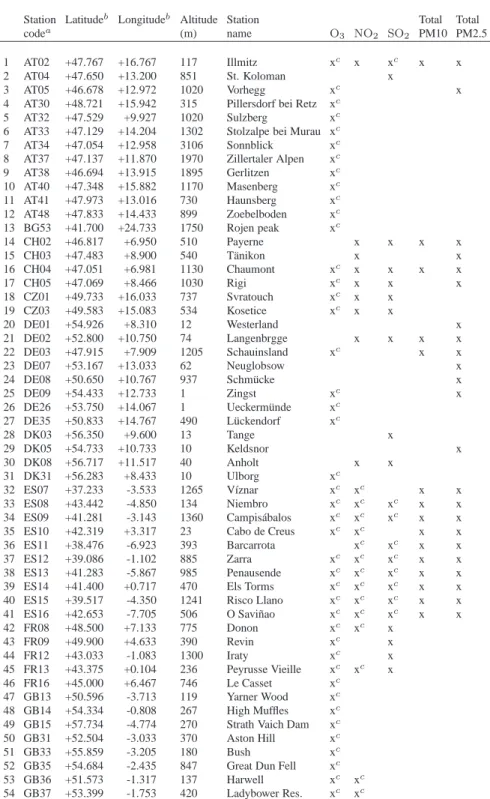
O3, 43 for NO2, 31 for SO2, 16 for PM2.5 and 25 for PM10, respectively. The 228
Figure 2: Grey shaded area: modeling domain used in this study. The white filled circles represent the selected subset of EMEP data collection sites. Characteristics of each station are listed in Table 1.
selected EMEP stations and measured pollutants that are used for this comparison
229
are briefly described in Table 1 and their locations are displayed in Fig. 2.
230
As EMEP aerosol measurements supposedly remove all water content from
231
samples to consider only dry aerosols, the simulated aerosol water was not taken
232
into account in the model-to-data comparisons. However, as noted by Tsyro
233
(2005), residual water persisting in sampled aerosols from EMEP may induce
234
a substantial underprediction by the simulated dry aerosol concentrations.
More-235
over, although the aerodynamic diameter is used for PM10 and PM2.5 in
measure-236
ment techniques, the model only considers the Stokes diameter to characterize the
237
aerosol geometry. For more details on this issue, see Jiang et al. (2006).
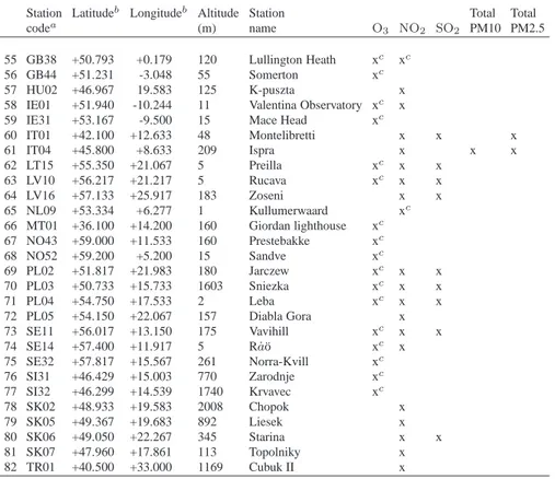
Table 1: Location and characteristics of selected EMEP stations for 2004 on a daily basis.
Station Latitudeb
Longitudeb
Altitude Station Total Total
codea (m) name O3 NO2 SO2 PM10 PM2.5 1 AT02 +47.767 +16.767 117 Illmitz xc x xc x x 2 AT04 +47.650 +13.200 851 St. Koloman x 3 AT05 +46.678 +12.972 1020 Vorhegg xc x 4 AT30 +48.721 +15.942 315 Pillersdorf bei Retz xc
5 AT32 +47.529 +9.927 1020 Sulzberg xc
6 AT33 +47.129 +14.204 1302 Stolzalpe bei Murau xc
7 AT34 +47.054 +12.958 3106 Sonnblick xc
8 AT37 +47.137 +11.870 1970 Zillertaler Alpen xc
9 AT38 +46.694 +13.915 1895 Gerlitzen xc 10 AT40 +47.348 +15.882 1170 Masenberg xc 11 AT41 +47.973 +13.016 730 Haunsberg xc 12 AT48 +47.833 +14.433 899 Zoebelboden xc 13 BG53 +41.700 +24.733 1750 Rojen peak xc 14 CH02 +46.817 +6.950 510 Payerne x x x x 15 CH03 +47.483 +8.900 540 T¨anikon x x 16 CH04 +47.051 +6.981 1130 Chaumont xc x x x x 17 CH05 +47.069 +8.466 1030 Rigi xc x x x 18 CZ01 +49.733 +16.033 737 Svratouch xc x x 19 CZ03 +49.583 +15.083 534 Kosetice xc x x 20 DE01 +54.926 +8.310 12 Westerland x 21 DE02 +52.800 +10.750 74 Langenbrgge x x x x 22 DE03 +47.915 +7.909 1205 Schauinsland xc x x 23 DE07 +53.167 +13.033 62 Neuglobsow x 24 DE08 +50.650 +10.767 937 Schm ¨ucke x 25 DE09 +54.433 +12.733 1 Zingst xc x
26 DE26 +53.750 +14.067 1 Ueckerm ¨unde xc
27 DE35 +50.833 +14.767 490 L ¨uckendorf xc 28 DK03 +56.350 +9.600 13 Tange x 29 DK05 +54.733 +10.733 10 Keldsnor x 30 DK08 +56.717 +11.517 40 Anholt x x 31 DK31 +56.283 +8.433 10 Ulborg xc 32 ES07 +37.233 -3.533 1265 V´ıznar xc xc x x 33 ES08 +43.442 -4.850 134 Niembro xc xc xc x x 34 ES09 +41.281 -3.143 1360 Campis´abalos xc xc xc x x
35 ES10 +42.319 +3.317 23 Cabo de Creus xc
xc x x 36 ES11 +38.476 -6.923 393 Barcarrota xc xc x x 37 ES12 +39.086 -1.102 885 Zarra xc xc xc x x 38 ES13 +41.283 -5.867 985 Penausende xc xc xc x x
39 ES14 +41.400 +0.717 470 Els Torms xc
xc xc
x x
40 ES15 +39.517 -4.350 1241 Risco Llano xc
xc xc x x 41 ES16 +42.653 -7.705 506 O Savi˜nao xc xc xc x x 42 FR08 +48.500 +7.133 775 Donon xc xc x 43 FR09 +49.900 +4.633 390 Revin xc x 44 FR12 +43.033 -1.083 1300 Iraty xc x 45 FR13 +43.375 +0.104 236 Peyrusse Vieille xc xc x 46 FR16 +45.000 +6.467 746 Le Casset xc 47 GB13 +50.596 -3.713 119 Yarner Wood xc 48 GB14 +54.334 -0.808 267 High Muffles xc
49 GB15 +57.734 -4.774 270 Strath Vaich Dam xc
50 GB31 +52.504 -3.033 370 Aston Hill xc
51 GB33 +55.859 -3.205 180 Bush xc
52 GB35 +54.684 -2.435 847 Great Dun Fell xc
53 GB36 +51.573 -1.317 137 Harwell xc xc
54 GB37 +53.399 -1.753 420 Ladybower Res. xc xc
Table 2: Continued.
Station Latitudeb
Longitudeb
Altitude Station Total Total
codea (m) name O3 NO2 SO2 PM10 PM2.5 55 GB38 +50.793 +0.179 120 Lullington Heath xc xc 56 GB44 +51.231 -3.048 55 Somerton xc 57 HU02 +46.967 19.583 125 K-puszta x
58 IE01 +51.940 -10.244 11 Valentina Observatory xc x
59 IE31 +53.167 -9.500 15 Mace Head xc
60 IT01 +42.100 +12.633 48 Montelibretti x x x 61 IT04 +45.800 +8.633 209 Ispra x x x 62 LT15 +55.350 +21.067 5 Preilla xc x x 63 LV10 +56.217 +21.217 5 Rucava xc x x 64 LV16 +57.133 +25.917 183 Zoseni x x 65 NL09 +53.334 +6.277 1 Kullumerwaard xc 66 MT01 +36.100 +14.200 160 Giordan lighthouse xc 67 NO43 +59.000 +11.533 160 Prestebakke xc 68 NO52 +59.200 +5.200 15 Sandve xc 69 PL02 +51.817 +21.983 180 Jarczew xc x x 70 PL03 +50.733 +15.733 1603 Sniezka xc x x 71 PL04 +54.750 +17.533 2 Leba xc x x 72 PL05 +54.150 +22.067 157 Diabla Gora x 73 SE11 +56.017 +13.150 175 Vavihill xc x x 74 SE14 +57.400 +11.917 5 R ˙a¨o xc x 75 SE32 +57.817 +15.567 261 Norra-Kvill xc 76 SI31 +46.429 +15.003 770 Zarodnje xc 77 SI32 +46.299 +14.539 1740 Krvavec xc 78 SK02 +48.933 +19.583 2008 Chopok x 79 SK05 +49.367 +19.683 892 Liesek x 80 SK06 +49.050 +22.267 345 Starina x x 81 SK07 +47.960 +17.861 113 Topolniky x 82 TR01 +40.500 +33.000 1169 Cubuk II x a
2-letter country code plus 2-digit station code.
b
A positive value indicates northern latitudes or eastern longitudes. A negative value indicates southern latitudes or western longitudes.
c
2.4. Statistical Indicators
239
There are a number of metrics that can be used to examine performances of
240
air quality models (U.S. EPA, 1984, 1991; Cox and Tikvart, 1990; Weil et al.,
241
1992; Chang and Hanna, 2004; Boylan and Russell, 2006). In particular, mean
242
normalized bias error (MNBE) and mean normalized gross error (MNGE)
nor-243
malizing the bias and error for each model-observed pair by the observation are
244
useful parameters. Correlation coefficient (r), root mean square errors (RMSE)
245
and mean bias (MB) values are also commonly used by the modeling community.
246
For the evaluation of particulate matter concentrations, Boylan and Russell (2006)
247
indicated that MNBE and MNGE may not be appropriate and suggested the mean
248
fractional bias (MFB) and the mean fractional error (MFE) parameters instead.
249
The US-EPA suggested several performance criteria for simulated O3, such 250
as MNBE ≤ ± 15% and MNGE ≤ 35% (U.S. EPA, 1991, 2007) whereas the
251
EC proposes a maximum uncertainty between measured and modeled
concentra-252
tions of 50% and 30% for O3/NO2/SO2 daily mean and NO2/SO2 annual mean, 253
respectively (European Commission, 2008). For particulate matter, Boylan and
254
Russell (2006) proposed that the model performance goal be met when both the
255
MFE and MFB are less than or equal to 50% and ± 30%, respectively, and the
256
model performance criterion be met when both MFE ≤ 75% and MFB ≤ 60%.
257
All these criteria and goals are selected to provide metrics for the CALIOPE-EU
258
model performances.
259
The model-to-data statistics MB, RMSE, MNBE, MNGE, MFB and MFE are
260
selected for the present study, together with the measured and modeled mean and
261
the correlation coefficient. Annual and seasonal mean statistics are computed,
262
with seasons corresponding to winter (January, February and December), spring
263
(March, April and May), summer (June, July and August) and fall (September,
264
October and November).
265
It is important to note that, unless explicitly stated otherwise, the statistical
266
norms are calculated without any minimum threshold when considering the
mea-267
surement data. However, in the present work, statistics of annual means using
268
thresholds are also computed. In that case we chose 80 µg m−3
for O3(according 269
to recommendations of the US-EPA, U.S. EPA, 1991; Russell and Dennis, 2000),
270 1.5 µg m−3 for NO2, 0.2 µg m −3 for SO2, 1.5 µg m −3 for PM10 and 3.5 µg m−3 271 for PM2.5, respectively. 272
3. Results and Discussion
273
As CALIOPE-EU is a fundamental model system the authors wish to stress
274
that, apart from the discussion of the Fig. 6 and its related statistics (Table 4),
275
neither correction factors nor any adjusting model parameterization were applied
276
to the model output or the original model codes. First, in Sect. 3.1, a thorough
277
model evaluation is performed through statistical and dynamical performances.
278
Later, in Sect. 3.2, a general description of the annual mean distribution of each
279
pollutant is provided to determine each pattern throughout Europe.
280
3.1. Model evaluation
281
Fig. 3 represents (left) the temporal series of the model (black lines) and daily
282
measured EMEP data (grey lines) as an average of all the stations for each
pol-283
lutant over the complete year 2004, together with (right) the scatterplot of the
284
modeled-measured daily data. Table 3 shows annual and seasonal statistics
cal-285
culated at the location of all EMEP stations. Statistics are calculated for daily
286
averages of O3, NO2, SO2, PM2.5 and PM10. In the case of O3, the daily peak of 287
hourly mean O3is also computed as it is one of the most important parameters to 288
be considered.
289
3.1.1. Ozone
290
A total of 60 EMEP stations constitute the O3measurement dataset to be com-291
pared to the simulation (see Table 1). In Fig. 3a, the time series of both simulated
292
and observed O3 concentrations are presented. The annual trend is well captured 293
with an annual correlation of daily mean and daily peak concentrations of 0.66
294
and 0.69, respectively (see Table 3). Although the annual daily mean bias is null,
295
the inter-annual variability leads to an annual RMSE of up to 20.6 µg m−3
.
An-296
nual and seasonal MNBE and MNGE values for daily mean and daily maximum
297
concentrations show relatively good performances which are in accordance with
298
the recommendations of the EC and the US-EPA (see Sect. 2.4).
299
Results show distinct inter-seasonal behaviors between colder and warmer
300
months. From January to March and from October to December, the model tends
301
to underestimate the mean concentrations (in winter, MB = -5.8 µg m−3), while
302
it slightly overestimates concentrations in summer months (MB = 7.5 µg m−3).
303
Correlation values are lowest for both daily mean and daily peak correlations in
304
the winter (r = 0.54 and 0.50, respectively). This inter-seasonal variability is
at-305
tributed to the model sensitivity to boundary conditions near the surface in winter.
306
During decreases of photochemical reactions in fall and winter the concentrations
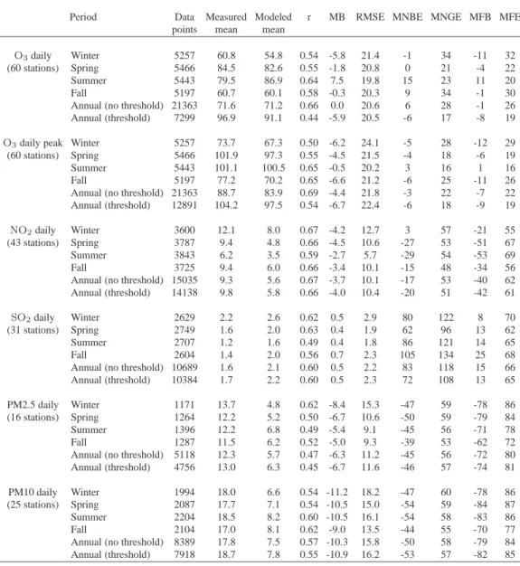
Table 3: Seasonal and annual statistics obtained with CALIOPE-EU over Europe for 2004 at the EMEP stations. Winter: January, February and December; Spring: March, April, May; Summer: June, July, August; Fall: September, October, November. The number of data points indicates the number of pair measurement-model used to compute the statistics. The calculated statistics are: measured mean for available data (µg m−3), modeled mean for the whole year (µg m−3),
correla-tion (r), Mean Bias (MB, µg m−3), Root Mean Square Error (RMSE, µg m−3), Mean Normalized
Bias Error (MNBE, %), Mean Normalized Gross Error (MNGE, %), Mean Fractional Bias (MFB, %) and Mean Fractional Error (MFE, %). For the annual mean calculated with threshold, we used 80 µg m−3for O
3, 1.5 µg m−3for NO2, 0.2 µg m−3for SO2, 1.5 µg m−3for PM2.5 and 3.5 µg
m−3for PM10, respectively. Seasonal statistics are computed without threshold.
Period Data Measured Modeled r MB RMSE MNBE MNGE MFB MFE
points mean mean
O3daily Winter 5257 60.8 54.8 0.54 -5.8 21.4 -1 34 -11 32
(60 stations) Spring 5466 84.5 82.6 0.55 -1.8 20.8 0 21 -4 22
Summer 5443 79.5 86.9 0.64 7.5 19.8 15 23 11 20
Fall 5197 60.7 60.1 0.58 -0.3 20.3 9 34 -1 30
Annual (no threshold) 21363 71.6 71.2 0.66 0.0 20.6 6 28 -1 26
Annual (threshold) 7299 96.9 91.1 0.44 -5.9 20.5 -6 17 -8 19
O3daily peak Winter 5257 73.7 67.3 0.50 -6.2 24.1 -5 28 -12 29
(60 stations) Spring 5466 101.9 97.3 0.55 -4.5 21.5 -4 18 -6 19
Summer 5443 101.1 100.5 0.65 -0.5 20.2 3 16 1 16
Fall 5197 77.2 70.2 0.65 -6.6 21.2 -6 25 -11 26
Annual (no threshold) 21363 88.7 83.9 0.69 -4.4 21.8 -3 22 -7 22
Annual (threshold) 12891 104.2 97.5 0.54 -6.7 22.4 -6 18 -9 19
NO2daily Winter 3600 12.1 8.0 0.67 -4.2 12.7 3 57 -21 55
(43 stations) Spring 3787 9.4 4.8 0.66 -4.5 10.6 -27 53 -51 67
Summer 3843 6.2 3.5 0.59 -2.7 5.7 -29 54 -53 69
Fall 3725 9.4 6.0 0.66 -3.4 10.1 -15 48 -34 56
Annual (no threshold) 15035 9.3 5.6 0.67 -3.7 10.1 -17 53 -40 62
Annual (threshold) 14138 9.8 5.8 0.66 -4.0 10.4 -20 51 -42 61
SO2daily Winter 2629 2.2 2.6 0.62 0.5 2.9 80 122 8 70
(31 stations) Spring 2749 1.6 2.0 0.63 0.4 1.9 62 96 13 62
Summer 2707 1.2 1.6 0.49 0.4 1.8 86 121 14 65
Fall 2604 1.4 2.0 0.56 0.7 2.3 105 134 25 68
Annual (no threshold) 10689 1.6 2.1 0.60 0.5 2.2 83 118 15 66
Annual (threshold) 10384 1.7 2.2 0.60 0.5 2.3 72 108 13 65
PM2.5 daily Winter 1171 13.7 4.8 0.62 -8.4 15.3 -47 59 -78 86
(16 stations) Spring 1264 12.2 5.2 0.50 -6.7 10.6 -50 59 -79 84
Summer 1396 12.2 6.8 0.49 -5.4 9.1 -45 56 -71 78
Fall 1287 11.5 6.2 0.52 -5.0 9.3 -39 53 -62 72
Annual (no threshold) 5118 12.3 5.7 0.47 -6.3 11.2 -45 56 -72 80
Annual (threshold) 4756 13.0 6.3 0.45 -6.7 11.6 -46 57 -74 81
PM10 daily Winter 1994 18.0 6.6 0.54 -11.2 18.2 -47 60 -78 86
(25 stations) Spring 2087 17.7 7.1 0.54 -10.5 15.0 -54 59 -84 87
Summer 2204 18.5 8.2 0.60 -10.5 16.1 -54 58 -83 86
Fall 2104 17.0 8.1 0.62 -9.0 13.5 -44 55 -70 77
Annual (no threshold) 8389 17.8 7.5 0.57 -10.3 15.8 -50 58 -79 84
defined at the boundaries proportionally acquire an increasing role in the control
308
of the concentration levels simulated within the domain. Also, the large
concentra-309
tions of O3in the highest layers of the boundary profile (reaching the stratosphere) 310
was found to be responsible for episodic inaccurate stratosphere-troposphere
ex-311
changes during colder months (not shown here; also see Eisele et al., 1999;
Cristo-312
fanelli and Bonasoni, 2009). Such finding was highlighted very recently by Lam
313
and Fu (2009) who pointed the inaccurate treatment of the tropopause in CMAQ
314
as the issue causing such artifact. On the other hand, the mean biases for daily and
315
daily peak concentrations are positive during warmer months with lowest RMSE
316
values (19.8 and 20.2 µg m−3 in summer, respectively). Model-observations
cor-317
relations, MNBE and MNGE values also reach the best values during this period.
318
This performance demonstrates the greater ability of the model to accurately
sim-319
ulate ozone during its intense photochemical formation in warmer months. Daily
320
variations are satisfactorily reproduced (see scatter plot in Fig. 3b with nearly 95%
321
of the data points falling within the 1:2 and 2:1 factor range). However, due to
un-322
certainties in the modeled nocturnal NOxcycle, the O3chemistry at night tends to 323
overpredict the observed concentrations. Such behaviour is partly reflected by the
324
difference between the annual mean biases calculated with or without the
mini-325
mum threshold of 80 µg m−3
on the measured data. By implementing this
thresh-326
old a part of overestimated nocturnal measured values is not considered which
327
induces a negative value of -5.9 µg m−3
compared to 0.0 using no threshold. For
328
extreme values (above 150 µg m−3
) the observed concentrations are
systemati-329
cally underestimated by the model (see Fig. 3b). This behavior is most likely
330
caused by high local pollution transported to rural sites but not captured with the
331
current horizontal resolution of the model (see Ching et al., 2006).
332
Fig. 4 and Fig. 5 present the spatial distributions in winter (left) and summer
333
(right) of the correlation and mean bias, respectively, without threshold on
mea-334
surements. In the case of O3 two different spatial regimes can be distinguished: 335
seasonal correlations are highest in England, central and southern Europe, while
336
Ireland and the countries along the North and Baltic Seas present lower
perfor-337
mances. We attribute these lower performances of the model at these locations
338
mostly to their relative proximity with the northern boundary of the domain. The
339
most remote sites with low levels of O3 display the lowest seasonal correlations 340
(see Irish and northern stations; from -0.2 to 0.2 in winter, from 0 to 0.4 in
sum-341
mer). The model skills improve notably from winter to summer as a result of the
342
increasing importance of the photochemical production of ozone. In summer most
343
of the seasonal correlations are comprised between 0.4 and 0.9. Also, statistics are
344
surprisingly satisfactory in complex regions such as the Alpine (stations CH02 to
CH05 and FR16) or the Pyrenean chains (FR12). As mentioned above in this
346
section the model tends to underestimate the mean concentrations in winter and
347
overestimate in summer (Fig. 5). It is noted that mean biases in southern Europe
348
have an inter-seasonal variability less pronounced than in the rest of Europe with
349
values rather positive. In summer, the lowest MB values are found in regions of
350
low mean O3levels such as the Alpine chain, Ireland and some Spanish stations. 351
3.1.2. Nitrogen Dioxide
352
As shown in Table 1, 43 stations were used to provide NO2 measurements 353
throughout Europe. The temporal and spatial variability of the simulated NO2 354
in Europe is larger than for O3, reflecting its higher sensitivity to meteorology 355
and model resolution (Vautard et al., 2009). The model-observations comparison,
356
presented in Fig. 3c and Fig. 3d highlights a correct annual trend, but with a
sys-357
tematic negative bias throughout the year. The dynamics is often well captured
358
but the amplitude of daily variations is underestimated. These low variations have
359
a direct impact on the daily variations of ozone in the PBL.
360
The annual average correlation is high (r=0.67, see Table 3), with better
per-361
formances in winter than in summer. Chemical processes, less dominant
com-362
pared to transport in winter, could explain such differences (Bessagnet et al.,
363
2004). Annual and seasonal mean biases are relatively high, ranging from -4.5
364
to -2.7 µg m−3
, leading to mean normalized error values rather near the
maxi-365
mum uncertainty proposed by the EC. High measured concentrations (above 70
366
µg m−3) are particularly underestimated (see Fig. 3d). When comparing modeled 367
results versus measured data, 59.1% of the corresponding data pairs fall within a
368
factor of 2 of each other, and 92.9% within a factor of 5.
369
The statistics of the model are spatially displayed in Fig. 4 and Fig. 5. NO2 370
concentrations are mostly driven by local to regional emissions. Therefore,
re-371
mote and clean boundary conditions are not significant contributors to the
sim-372
ulated concentrations of NO2 in Europe. Correlations are highest in winter for 373
the areas including UK, northern countries and some spanish stations. In these
re-374
gions emissions of NOxare generally either high or very low (also see Sect. 3.2.2). 375
Low correlations are mainly concentrated in central Europe (coefficients between
376
-0.2 and 0.4). Numerous stations located in low-NO2 areas display satisfactory 377
seasonal mean biases (see northern and central Europe and Spain with seasonal
378
MB= ± 2 µg m−3), while stations substantially affected by transport from source
379
regions display the highest seasonal mean biases (Fig. 5). The aforementioned
380
large underestimations of high measured concentrations are mainly caused by the
381
three stations from Great Britain (GB36, GB37 and GB38, see Table 1). These
stations frequently undergo high pollution events caused by emissions from road
383
traffic and combustion processes. To a lesser extent, these highly polluted plumes
384
from the United Kingdom (UK) also affect the measuring station in The
Nether-385
lands (NL09) under westerly winds and contribute to the increase in mean bias
386
values when the transport is not accurately simulated. At these locations, negative
387
mean biases reaching up to 22 µg m−3
on annual average are noted with highest
388
biases in winter. Such differences are most likely caused by the underestimation
389
of emission sources in these areas. Altogether, the analysis of the spatial
distri-390
bution of the model skills shows that the level NO2 concentrations at very rural 391
stations is well captured but with low correlation coefficients, while mean biases
392
and correlation coefficients are greatest at polluted stations.
393
Apart from sources unaccounted for in the emission database, uncertainties
394
may also arise in the spatial and temporal distribution of the sources (Stern et al.,
395
2008). In the PBL NOxconcentrations are dominated by emissions near the sur-396
face, such as traffic and domestic heating, which are subject to strong spatial and
397
temporal variations.
398
3.1.3. Sulfur Dioxide
399
For SO2, the model results were evaluated against 31 EMEP stations mea-400
suring daily mean concentrations of SO2 at background sites. The stations are 401
located across the Iberian Peninsula, central and north-eastern Europe. It is worth
402
noting that the daily mean concentrations are low and provide information about
403
the background levels of SO2 across Europe only. Fig. 3e shows the time series 404
of the daily mean concentrations of SO2 at the EMEP stations together with the 405
model simulation at these stations. Results show that SO2concentrations are well 406
captured by the model, although some observed peaks are overestimated. During
407
the cold months (January, February, March, October, November) the model agrees
408
well with observations, and monthly variations of SO2 are well captured. On the 409
other hand, during the warm period (April, May, June, July, August and
Septem-410
ber) results present an overall positive bias of 1 µg m−3. September and December
411
months are characterized by some episodes of large overestimations. Overall, the
412
dynamical evolution of the model is in good agreement with the observations. For
413
instance, January undergoes two major episodes of enhanced SO2 that the model 414
reproduces well. Although there is a clear overestimation during some periods,
415
the model is able to reproduce the variations of the daily mean concentrations.
416
As regard to the scatter plot (Fig. 3f), 54.3% of the model results match with
417
observations within a factor of 2, and 90.1% within a factor of 5. The model
re-418
sults match the main tendency of the daily observations with an annual correlation
factor r=0.60.
420
The annual mean MNGE and MNBE values reach up to 118% and 83%
re-421
spectively (Table 3). Such rather high normalized errors are usual when
evaluat-422
ing background stations that measure very low values of SO2. The annual RMSE 423
is 2.2 µg m−3
, much lower than for the other pollutants analyzed in the present
424
work. The seasonal statistics show better results for spring, with mean MNGE
425
value of 96%. The MNBE values increase for summer and fall as the daily mean
426
observations remain below 2 µg m−3.
427
The spatial distribution of the correlation coefficient r shows a large
variabil-428
ity per station. For instance, during winter while some northern stations have
429
high correlations (0.6 < r < 0.9), various low correlations are observed in central
430
and southern Europe. During summertime the correlation improves in stations
lo-431
cated over central Europe. In Spain, the model performs relatively homogeneously
432
across the year, with a variation of the correlation between summer and winter less
433
pronounced than in central Europe. However, the correlation per station in Spain
434
is slightly lower than in the rest of Europe, especially during summer.
435
Considering the mean bias for winter and summer (Fig. 5), results show a low
436
bias across all stations. Only one station located in eastern Poland displays a high
437
positive bias (> 5 µg m−3
in summer). This station may largely contribute to the
438
seasonal and annual average positive bias mentioned in Table 3. The uncertainties
439
of the emission inventory in eastern Europe may be associated to the higher bias
440
observed in some stations of Poland and the Czech Republic, especially in winter.
441
Also, the top-down disaggregation from 50 to 12 km is a source of uncertainties
442
to be considered.
443
3.1.4. Particulate matter
444
A total of 16 and 25 stations are used to evaluate the simulated PM2.5 and
445
PM10 concentrations, respectively. Although the model presents a clear
sys-446
tematic negative bias, it has noticeable capabilities to reproduce the dynamics
447
of PM2.5 for the whole year (Fig. 3g). The modeling system simulates the most
448
important PM2.5 episodes across the whole year. The correlation coefficients
449
for winter and fall seasons are 0.62 and 0.52, respectively, and 0.50 and 0.49 for
450
spring and summer (Table 3). The MFE and MFB for PM2.5 do not fall within the
451
performance criteria or performance goal proposed by Boylan and Russell (2006).
452
In order to evaluate the annual variability of PM in comparison to
measure-453
ment data, Fig. 6 displays the annual time series of PM2.5 and PM10 multiplied
454
by a correction factor of 2. Such correction is not meant to modify the statistics
455
but rather to evaluate the annual dynamics of the model and approximate the
Table 4: Seasonal and annual statistics obtained with CALIOPE-EU over Europe for 2004 (see Table 3). For quantification purposes, the simulated concentrations of PM are multiplied by a correction factor of 2 at the EMEP stations.
Period Data Measured Modeled r MB RMSE MNBE MNGE MFB MFE
points mean mean
PM2.5 daily Winter 1171 13.7 9.6 0.62 -3.3 12.4 6 60 -20 58
adapted (×2) Spring 1264 12.2 10.4 0.50 -1.3 10.0 1 49 -19 47
(16 stations) Summer 1396 12.2 13.6 0.49 1.3 13.0 10 52 -10 45
Fall 1287 11.5 12.3 0.52 1.5 11.4 22 58 -1 47
Annual (no threshold) 5118 12.3 11.5 0.47 -0.3 11.8 10 54 -12 49
Annual (threshold) 4756 13.0 12.6 0.45 -0.4 12.2 7 53 -14 49
PM10 daily Winter 1994 18.0 13.3 0.54 -4.3 14.7 6 61 -21 57
adapted (×2) Spring 2087 17.7 14.2 0.54 -3.4 12.4 -7 46 -25 48
(25 stations) Summer 2204 18.5 16.3 0.60 -2.4 14.8 -7 46 -23 49
Fall 2104 17.0 16.1 0.62 -0.9 12.1 13 56 -10 49
Annual (no threshold) 8389 17.8 15.0 0.57 -2.7 13.6 1 52 -20 51
Annual (threshold) 7918 18.7 15.6 0.55 -3.1 13.9 -5 48 -23 50
derestimation of PM mass. By multiplying the model results by such a factor, the
457
results of the model system are in very good agreement with observations. The
458
model is able to reproduce the daily evolution of PM2.5 across the year.
Neverthe-459
less, the model tends to underestimate the peaks during wintertime, while during
460
summertime the model overestimates some episodes. By calculating the annual
461
MFE and MFB with the adapted model output, the results now fall within the
462
performance goal recommended by Boylan and Russell (2006) with a MFE=49%
463
and MFB=-12% (Table 4). It is important to note that the statistics are biased
464
towards measurements obtained in Spain, since 10 out of 16 EMEP stations are
465
located there (Fig. 4 and Fig. 5). Overall, the MFB and MFE are homogeneous at
466
most stations (not shown).
467
For PM10, annual correlations are higher than for PM2.5 (annual mean
cor-468
relation r=0.57). The model is able to reproduce most of the particulate matter
469
events, although the model hardly reproduces the amplitude of the events and
470
presents a systematic underestimation. Concerning the variability of the results
471
(Fig. 3j), 69.4% of the data match with observations within a factor 2, and 96.6%
472
within a factor 5. As for PM2.5, PM10 results present a very good agreement with
473
the observations if a factor of 2 is applied to the results (Fig. 6b). The adapted
re-474
sults for PM10 match consistently with the observations except for the Saharan
475
dust outbreak event on July 24-26th which affected southern, central and eastern
Spain but was not captured by BSC-DREAM8b.
477
The annual mean MFB and MFE of the adapted results amount to -20% and
478
51%, respectively (Table 4). These results are in accordance with the
recom-479
mendations for particulate matter mentioned in Sect. 2.4 and fall within the
per-480
formance criteria of Boylan and Russell (2006). The spatial distribution of the
481
correlation coefficient and the mean bias for winter and summer point out that
482
the model performs better in southern than in northern Europe, for PM10 (Fig. 4
483
and Fig. 5). Stations located between the Baltic and the North Sea (DE01, DE09,
484
DK05; see Table 1) display weak seasonal correlation coefficient (-0.1 < r < 0.3).
485
However, continental stations of central Europe (Germany, Switzerland and
Aus-486
tria) mainly affected by anthropogenic emissions present good performances for
487
PM10. Correlations are in the range of 0.3-0.7 during winter and improves in
488
summer. From all coastal sites affected by SSA, the stations in Spain display the
489
highest correlations (Niembro and Cabo de Creus with 0.4 < r < 0.6). At the
490
south European stations affected by Saharan dust outbreaks, namely Spain and
491
Italy, correlations are high across the year (0.5 < r < 0.9, except ES13). The
492
inclusion of BSC-DREAM8b model results largely contributes to the
improve-493
ment of the model performances at such southern stations as previously noted by
494
Jim´enez-Guerrero et al. (2008).
495
Many studies have recognized the difficulty of models to simulate the mass
496
of particulate matter over Europe (van Loon et al., 2004; Matthias, 2008). The
497
underestimation of total particulate mass is, among others, the result from the lack
498
of fugitive dust emissions, resuspended matter (Vautard et al., 2005a), a possible
499
underestimation of primary carbonaceous particles (Schaap et al., 2004; Tsyro,
500
2005), the inaccuracy of SOA formation (Simpson et al., 2007), the difficulty of
501
representing primary PM emission from wood burning and other sources (Tsyro
502
et al., 2007) and a more general lack of process knowledge (Stern et al., 2008).
503
While multiplying the model results of CALIOPE-EU by a factor of 2, it was
504
shown that the dynamics of particulate matter (both PM2.5 and PM10) can be well
505
captured. Using such methodology the levels generally simulated by
CALIOPE-506
EU were quantified to be approximately half of the observed values.
507
3.2. Pattern Description
508
In the following section, it is important to note that the description of the
509
simulated chemical patterns does not take into account the model-observations
510
discrepancies highlighted in Sect. 3.1.
3.2.1. Ozone
512
Modeled O3average concentrations over Europe (Fig. 7a) show an increasing 513
gradient from the northern and western boundaries to the more continental and
514
Mediterranean areas, resulting from large variations in climate patterns (Beck and
515
Grennfeld, 1993; Lelieveld et al., 2002; EEA, 2005; Jim´enez et al., 2006). In the
516
troposphere O3 has a residence time of several days to a week which permits its 517
transport on regional scales (Seinfeld and Pandis, 1998). The highest
concentra-518
tions are found in the Mediterranean basin and southern Europe (nearly 90-105 µg
519
m−3), as this region is particularly affected by intense photochemical production
520
of O3 (EEA, 2005; Vautard et al., 2005b). Detailed descriptions of ozone for-521
mation and transport over the Mediterranean area can be found in Gerasopoulos
522
et al. (2005) or Cristofanelli and Bonasoni (2009). Other important factor for the
523
land-sea difference is the slow dry deposition of O3on water and also the low pho-524
tochemical formation due to the low precursors concentration (Wesely and Hicks,
525
2000) . In central and eastern Europe, simulated annual O3 concentrations range 526
from 70 to 85 µg m−3
, with a slight west-to-east gradual build-up caused by the
527
association of precursor emissions and predominant westerly winds.
Northwest-528
ern areas show rather low concentrations of O3 (60-67 µg m −3
) due to reduced
529
solar radiation and the influence of the clean marine air. Due to higher O3 con-530
centrations in elevated terrains, the major mountainous regions such as the Alpine
531
and Pyrennean chains as well as the Carpathian mountains (mainly in Rumania)
532
display mean O3 concentrations in the range of 85-95 µg m −3
. The minimum
533
values of O3(50-55 µg m −3
) are found in regions of chemically-driven high-NOx 534
regime such as large polluted cities or within the shipping routes, Great Britain
535
and The Netherlands, and in northernmost Europe due to the association of low
536
precursor emissions and polar-like weather types. The O3 distribution described 537
in this section is in accordance with the EMEP model results for the year 2005
538
presented by Tarras´on et al. (2007). However, the rather coarse resolution used
539
by the EMEP model (50 km × 50 km) led to a less accurate simulation of the
540
chemical transition between urban and background areas.
541
3.2.2. Nitrogen dioxide
542
High concentrations of NO2 within the PBL are directly related to anthro-543
pogenic emissions (EEA, 2007). The largest contributors to NO2 atmospheric 544
concentrations are the emissions from road transport (40% of NO2total emission) 545
followed by power plants and other fuel converters (22% of NO2 total emission, 546
Tarras´on et al., 2006). High modeled NO2 concentrations (∼ 20-30 µg m −3
)
547
are reported in The Netherlands and Belgium, the industrial Po Valley (northern
Italy), central and eastern England, and the Ruhr region (western Germany).
Var-549
ious important European cities even reach NO2 levels up to 30-40 µg m −3
on
550
annual average (e.g., Milan, London, Paris). Suburban areas surrounding the
ma-551
jor cities often undergo advections of polluted air masses and display mean annual
552
values near 10-25 µg m−3
while clean regions unaffected by emissions rather have
553
concentrations below 5 µg m−3
. Also note that the major shipping routes
originat-554
ing from the North Sea, passing by the English Channel, through Portugal, Spain
555
and northern Africa toward the Suez Canal substantially affect the coastal NO2 556
concentrations with a maximum of 18 µg m−3 for the annual mean
concentra-557
tions. Qualitative comparisons between the simulated pattern of annual NO2and 558
satellite-derived NO2 tropospheric column densities from GOME (Beirle et al., 559
2004), SCIAMACHY and OMI (Boersma et al., 2007) revealed good agreement
560
(not shown). Such finding demonstrates the relative accuracy in the spatial
de-561
scription of the source regions and various European hot-spots.
562
3.2.3. Sulfur dioxide
563
Simulated SO2 annual average concentrations over Europe (Fig. 7c) show 564
highest levels over northwestern Spain, eastern Europe (Poland, Serbia, Rumania,
565
Bulgaria and Greece), and over UK, Belgium and the southwestern part of The
566
Netherlands. Combustion emissions from power plants and transformation
indus-567
tries are the main responsible for such high concentrations of SO2 over Europe. 568
64% of SO2 total emissions are attributed to these sectors (Tarras´on et al., 2006). 569
The highest annual concentrations (∼70-90 µg m−3
) are observed in northern
570
Spain due to the presence of two large power plant installations. However,
back-571
ground regions in Spain remain below mean concentrations of 2 µg m−3
. On the
572
other hand, east European countries are affected by higher background
concentra-573
tions of SO2(∼8 to 20 µg m −3
) with various punctual emissions contributing to an
574
increase of the regional concentrations (∼30 to 50 µg m−3). Over sea, the highest
575
concentrations are found along the main shipping routes, as emissions from ships
576
largely contribute to the SOxconcentrations due to combustion of fuels with high 577
sulfur content (Corbett and Fischbeck, 1997; Corbett and Koehler, 2003).
578
The distribution of mean annual SO2concentrations for 2004 shows the same 579
pattern as that presented by Tarras´on et al. (2007) for 2005. However, note that the
580
SO2 levels have decreased according to the pattern shown in Schaap et al. (2004) 581
for the year 1995. Indeed, from the mid-1990s to 2004, SO2concentrations in air 582
have strongly decreased due to reductions in SOxemissions. SOxemissions have 583
reduced up to 50% mainly in the sectors of power and heat generation through
584
a combination of using fuels with lower sulfur content (such as switching from
coal and oil to natural gas) and implementing emission abatement strategies in the
586
energy supply and industry sectors (EEA, 2007; International Maritime
Organiza-587
tion and Marine Environment Protection Committee, 2001).
588
3.2.4. Particulate matter
589
The simulated spatial distribution of annual mean PM2.5 (Fig. 7d) shows
av-590
erage background levels around 3-10 µg m−3
in northwestern, central and eastern
591
Europe. Very low concentrations correspond to remote marine air and the
ma-592
jor European mountain chains (e.g., the Alps, Massif Central, the Pyrenees and
593
the Carpathians). The concentration levels are dominated by SIA, namely sulfate,
594
nitrate and ammonium (not shown here). SSA does not substantially contribute
595
to the PM2.5 fraction. The most polluted European region is the Po Valley with
596
annual mean values near 14-22 µg m−3. To a lesser extent, in the Benelux
re-597
gion (Belgium, The Netherlands, Luxembourg) high concentrations of PM2.5 are
598
found (∼8-12 µg m−3). Such concentrations are mainly associated with primary
599
anthropogenic emissions from road traffic and secondary aerosols. As mentioned
600
in Sect. 3.2.3 Bulgaria, Rumania and Poland are important contributors of SO2. 601
At the hot-spot locations, the large sulfate formation and primary PM emissions
602
lead to annual mean concentrations of up to 20-22 µg m−3. Interestingly, the large
603
sources of SO2 located in eastern UK and northwestern Spain do not contribute 604
efficiently to the PM2.5 formation. Such low sulfate formation is most likely
605
caused by high dispersion and strong removal by wet deposition in these regions.
606
The north African continent constitutes a very large potential source of PM for
607
the rest of the domain. During episodes of Saharan dust outbreaks, mineral dust
608
largely contributes to the levels of PM2.5 in southern Europe.
609
Fig. 8a and Fig. 8b present the annual mean and 1-hour maximum of PM10
610
concentrations in Europe, respectively. PM10 includes the PM2.5 fraction, the
611
primary anthropogenic coarse fraction (PM10−2.5), as well as the contribution of 612
coarse SSA and Saharan dust. Among other uncertainties, wind-blown or
re-613
suspended dust emissions (coarse fraction) are not taken into account yet. Such
614
sources contribute to the underestimation of the total concentrations of PM10,
615
especially in dry regions or in urban areas (see Amato et al., 2009a,b).
616
High mean and maximum values of annual PM10 concentrations found in the
617
North Sea and the nearshore Atlantic result from SSA production. The mean
con-618
tribution of SSA in the Mediterranean Sea reaches around 10 µg m−3. The annual
619
mean contribution of the anthropogenic coarse fraction remains low (∼5 µg m−3
)
620
and is located at or in the vicinity of important emission sources (not shown).
Sa-621
haran dust is responsible for the very high levels of PM in northern Africa and
also regularly affects the Mediterranean basin and southern Europe. Spain,
south-623
ern France, Italy, and Greece are particularly affected by such episodes. Fig. 8b
624
reflects well the importance of including Saharan dust model data (on a
non-625
climatic basis) since dust outbreaks lead to annual maximum concentrations of
626
PM10 greater than 300 µg m−3
in most of the territories surrounding the
Mediter-627
ranean Sea.
628
Qualitatively, the spatial distributions of PM2.5 and PM10 show similar
pat-629
terns to distributions found in other European modeling studies including sea salt
630
and Saharan dust emissions (see, e.g., POLYPHEMUS and the Unified EMEP
631
model, Sartelet et al., 2007; Tarras´on et al., 2006). Substantial differences arise
632
in concentrations over southern Europe when comparing spatial distributions with
633
models not taking dust from the African continent into account (see Bessagnet
634
et al., 2004).
635
4. Comparison with Other Evaluation Studies
636
There are several air pollution modeling systems on the European scale
op-637
erated routinely in Europe. Evaluations of these regional air quality models with
638
ground-based measurements were carried out either individually or in
compari-639
son to other models. The following discussion presents a comparative analysis
640
between various European model evaluations and CALIOPE-EU. This analysis
641
does not attempt to be an intercomparison study because the studies were
per-642
formed under different conditions (simulated year, meteorological data, boundary
643
conditions, emissions, etc.). However, it provides a good basis for assessing the
644
reliability of the results obtained in the context of the European evaluation
mod-645
els. Table 5 shows a chronological list of published evaluation studies, which are
646
presented along with CALIOPE-EU evaluation results.
647
The presented evaluation studies have several characteristics in common. First,
648
they were carried out over Europe on a regional scale with horizontal resolutions
649
in the range of 25-55 km × km. Second, the simulations were run over a long
650
period, mainly a year. The given models were evaluated against ground-based
ob-651
servations at rural locations from EMEP or AIRBASE databases. Also note that
652
these evaluation studies were performed using statistical methods.
653
Most of the studies presented here, evaluated independently in previous
pub-654
lications, focused on both gas and particulate phases. These studies comprise:
655
LOTOS-EUROS (Schaap et al., 2008), POLYPHEMUS (Sartelet et al., 2007),
656
Unified EMEP (Tarras´on et al., 2006; Yttri et al., 2006), and CHIMERE
(Bessag-657
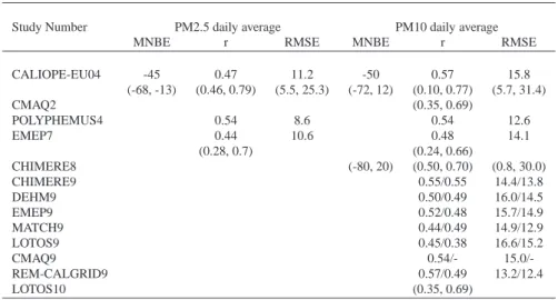
net et al., 2004; Schmidt et al., 2001). In the case of the Unified EMEP model,
Table 5: List of published European model evaluation studies and their main characteristics to be compared with CALIOPE-EU evaluation results (this study). A study code for each model is specified to ease the discussion in this paper.
Reference Modeled Model Horizontal resolution Study code
year name /layers
This study 2004 CALIOPE-EU 12 km×12 km/15 CALIOPE-EU04
Matthias (2008) 2001 CMAQ 54 km×54 km/20 CMAQ2
Schaap et al. (2008) 1999 LOTOS-EUROS 25 km×25 km LOTOS-EUROS3
Sartelet et al. (2007) 2001 POLYPHEMUS 0.5◦×0.5◦/5 POLYPHEMUS4 van Loon et al. (2007) 1999 Unified EMEP 50 km×50 km/20 EMEP5
van Loon et al. (2007) 1999 RCG 0.5◦×0.5◦/5 RCG5
van Loon et al. (2007) 1999 LOTOS-EUROS 0.5◦×0.5◦/4 LOTOS-EUROS5 van Loon et al. (2007) 1999 CHIMERE 0.5◦×0.5◦/8 CHIMERE5
van Loon et al. (2007) 1999 MATCH 0.4◦×0.4◦/14 MATCH5
Tarras ´on et al. (2006) 2004 Unified EMEP 50 km×50 km/20 EMEP6 Yttri et al. (2005) 2004 Unified EMEP 50 km×50 km/20 EMEP7 Bessagnet et al. (2004) 1999 CHIMERE 0.5◦×0.5◦/8 CHIMERE8 van Loon et al. (2004) 1999/2001 CHIMERE 0.5◦×0.5◦/8 CHIMERE9 van Loon et al. (2004) 1999/2001 DEHM 50 km×50 km/20 DEHM9 van Loon et al. (2004) 1999/2001 Unified EMEP 50 km×50 km/20 EMEP9 van Loon et al. (2004) 1999/2001 MATCH 55 km×55 km/10 MATCH9 van Loon et al. (2004) 1999/2001 LOTOS 0.25◦×0.5◦/3 LOTOS9 van Loon et al. (2004) 1999/2001 CMAQ 36 km×36 km/21 CMAQ9 van Loon et al. (2004) 1999/2001 REM-CALGRID 0.25◦×0.5◦ REM-CALGRID9
Schaap et al. (2004) 1995 LOTOS 25 km×25 km/3 LOTOS10
Hass et al. (2003) 1995 DEHM 50 km×50 km/10 DEHM11
Hass et al. (2003) 1995 EURAD 27 km×27 km/15 EURAD11
Hass et al. (2003) 1995 EUROS 0.55◦×0.55◦/4 EUROS11
Hass et al. (2003) 1995 LOTOS 0.25◦×0.5◦/3 LOTOS11
Hass et al. (2003) 1995 MATCH 55 km×55 km/10 MATCH11
Hass et al. (2003) 1995 REM3 0.25◦×0.5◦ REM11