Worlds apart: what polarization measures reveal about Sub-Saharan Africa's growth and welfare distribution in the last two decades

(1)

1

Worlds Apart: What polarization measures reveal about

Sub-Saharan Africa’s growth and welfare distribution

in the last two decades

F. Clementia_{, M. Fabiani}a_{, V. Molini}b,*_{, and R. Zizzamia}c a_{University of Macerata, Macerata, Italy}

b_{World Bank, Washington DC, USA}

c_{Southern African Labour and Development Research Unit, University of Cape Town, Cape}

Town, South Africa

April 24, 2019

Abstract

Sub-Saharan Africa’s development path over the past two decades has been characterized by sluggish poverty reduction occurring alongside robust economic growth. While in this context we would expect inequality to increase, standard synthetic measures provide little evidence of a generalizable uptick in inequality over this period. We argue that the standard empirical toolkit available to development economists working on SSA has limited our ability to understand the role that distributional change plays in the persistence and reproduction of poverty on the continent. For this reason, we propose that supplementing inequality measures with the analysis of polarization provides a cleaner distributional lens through which to make sense of SSA’s poverty performance during this period of growth. Applying polarization measures to comparable survey data from 24 Sub-Saharan African countries, we find that there has been a generalizable increase in polarization over the past two decades – and in particular, an increased concentration of households in the lower tail of the relative distribution. That this inegalitarian trend is overlooked when using standard synthetic inequality measures confirms our hypothesis that our current toolkit represents a technical bottleneck to understanding the effects of distributional trends on poverty reduction in Sub-Saharan Africa – and that polarization analysis may help overcome this.

Keywords: Sub-Saharan Africa; consumption distribution; polarization; relative distribution; decomposition analysis. JEL classification: C14; D31; D63; I32.

*_{Corresponding author. Email addresses:}_{fabio.clementi@unimc.it}_{(F. Clementi),}_{m.fabiani9@unimc.it}_{(M. Fabiani),}

(2)

2

1 Introduction

Over the last twenty years, Sub-Saharan Africa (SSA) has experienced an unprecedented resurgence of economic growth. While this growth is encouraging for the prospects of SSA’s economic development (Fosu, 2018; Dollar and Kraay, 2002; Ravallion, 2001), a debate is ongoing regarding its nature and outcomes. In particular, scholars have questioned the extent to which this growth has been driven by the structural transformation of African economies away from agriculture and into services and manufacturing, or, alternatively, by fortuitous and potentially temporary favorable external conditions (Diao et al., 2018; Rodrik, 2016; Bhorat et al., 2017). To the extent that growth has been driven by external conditions such as a rise in commodity prices and low interest rates, there are concerns that SSA’s poor performance in translating growth into poverty reduction is symptomatic of the fragility and unsustainability of SSA’s growth trajectory (Beegle et al., 2016; World Bank, 2018).

It is now generally agreed that, while most countries in SSA have experienced reductions in poverty, this progress has been relatively slow compared to other non-African developing countries experiencing similar growth rates (Thorbecke and Ouyang, 2018). An intuitive explanation for this sub-optimal performance is given by the abundant literature on growth non-inclusiveness in SSA (inter alia Christiansen et al., 2013; Cornia, 2015; Odusola et al., 2017). Most scholars have made sense of SSA’s post-colonial growth experience by arguing that growth at the top of the distribution can be characterized as “rent-seeking”, i.e. driven by rising rents from resource extraction as the form and function of extractive institutions from a colonial past have been maintained (Devarajan et al., 2013; Knight, 2015; Atkinson, 2014). In a nutshell, economic growth, when driven by a resource boom and presided over by extractive institutions, disproportionately benefits a country’s ruling elite rather than the poor (Acemoglu and Robinson, 2012; Sala-i-Martin and Subramanian, 2003; Robinson et al., 2006; Devarajan et al., 2013). Consequently, many have observed that the growth pattern in SSA has remained unevenly distributed, and, as in the West, has largely failed to “trickle down” to the poor.

The inequality performance in SSA, we also argue, raises questions regarding development theory, the application of which would predict a systematic increase in inequality over the last two decades (Beegle et al., 2016). Literature on the topic (inter alia Lewis, 1955; Gollin et al., 2014) has noted that, even during the recent economic take-off, large productivity gaps between

(3)

3

agriculture and non-agricultural sectors have persisted (MacMillan et al., 2014). The persistence of these gaps also has an important spatial dimension relevant to inequality, since many SSA economies appear to be highly dualistic, displaying enduring rural-urban divides in terms of human capital, infrastructure and economic opportunity (Molini and Paci, 2015; World Bank, 2016). According to the Kuznets’ curve theory (Kuznets, 1955; Kanbur, 2017), inequality first increases and then declines as a country develops. In SSA, the low initial level of development as well as persistent sectoral and spatial productivity gaps would predict an increase in income differentials during the early growth spurt. However, as mentioned before, inequality figures from SSA fail to provide strong evidence for a Kuznets-type trajectory. Although there is a significant positive relationship between the level of GDP and inequality (Bhorat et al., 2016; Beegle et al., 2016), this is driven almost entirely by those countries in the Southern cone.

From the above, we would expect that high and increasing inequality is the immediate culprit for SSA’s comparatively poor record in translating growth into poverty reduction over the last twenty years. However, the evidence in this regard is rather scattered and ambiguous. While SSA is frequently said to rival Latin America as the most unequal region in the world, this is driven by the few exceptionally unequal countries in the continent’s Southern cone (Odusola et al., 2017). Excluding the Southern cone, inequality in SSA is not high by developing country standards. Evidence of recent trends in inequality during the SSA’s growth miracle is also mixed – no clear pattern emerges which could hold generally across the continent.

Pinhovskiy and Sala-i-Martin (2014) show that the recent growth spurt was, in fact, accompanied by a generalized decrease in inequality. Beegle et al. (2016) find that, of 23 countries where data is available to track changes in inequality, half can be shown to have experienced increases in inequality, while the other half experienced decreases. Odusola et al. (2017) also find a bifurcation in inequality trends in SSA: 17 countries experienced declining inequality, whereas 12 countries, predominantly in Southern and Central Africa, recorded an inequality rise. While in the African context there are clearly data limitations, it is relevant that those studies relying on comparable survey data (such as Beegle et al., 2016) find no evidence of a generalized increase in inequality. Therefore, these studies provide no reason to suggest that inequality (either regarding trends or initial conditions) is a sufficient explanation for SSA’s poor performance in reducing poverty commensurately with growth.

Searching for possible explanations for this conundrum, this paper questions the capacity of standard measures of inequality (such as the commonly used Gini coefficient) to reflect those

(4)

4

distributional changes occurring in SSA which are most relevant to poverty reduction (Clementi et al., 2019). This admits of two possibilities: First, that standard measures underestimate inequality increases in the region, and, second, that standard measures fail to illuminate with sufficient granularity the distributional patterns which matter most for poverty reduction (whether or not there is an aggregate increase in inequality).

In undertaking this investigation, we show that polarization analysis methods reveal that distributional changes had a clear inegalitarian pattern throughout the region. Further, we argue that these trends are best detected when using polarization analysis methods, which have the advantage of allowing us to pinpoint where in the distribution relevant changes have occurred. To complete the exercise, we investigate the drivers of this polarization process. These may be due to changes in observable characteristics (such as an increase in mean levels of education) or in returns to characteristics (such as changes in the returns to education in the labor market). We do this by running an unconditional quantile regression (Firpo et al., 2009), which allows us to single out the effect of different covariates of polarization at different points in the consumption distribution.

The rest of the paper is organized as follows. Section 2 briefly describes the advantages and disadvantages of inequality and polarization measures. Section 3 details the methods used to produce our results. Section 4 presents the data used. Section 5 presents the empirical results. Finally, Section 6 concludes.

2 Inequality vs Polarization

As mentioned, when measured with standard indicators like the Gini or the Theil index, there is no clear evidence of an increase in inequality in the last two decades (Figure 1, on the next page). Regarding the Gini, 11 countries experienced a decline and 13 a rise, while for the Theil, 13 saw a decline and 11 a rise – yet in case of the Theil in 10 out 24 countries considered this variation is not statistically significant. Therefore, it is difficult to identify a generalizable pattern among SSA countries in terms of inequality trends over time. Odusola et al. (2017) have characterized the region’s overall inequality trajectory as “inequality bifurcation”. It remains possible, however, that important and generalizable distributional changes occurred over the last two decades, and yet went largely undetected by standard inequality measures such as the Gini or Theil indices.

(5)

5

Since inequality indices provide summary measures of the overall dispersion of a distribution, in practice this means that a pro-inequality change in one part of the distribution may be compensated by a pro-equality change in another part of the distribution. However, the dynamic measurement of inequality using the Gini, for example, is more sensitive to distributional changes in the center of the distribution than it is to changes in the tails.

A rich literature on inequality measurement has produced several alternative inequality indices that overcome some of the limitations of the Gini – including the fact that dynamic measurement of inequality using the Gini puts most weight on changes in the middle of the distribution. The generalized entropy (GE) class of inequality measures, for instance, provides a full range of bottom- to top-sensitive indices depending on the value assigned to the parameter that characterizes the sensitivity of the GE index to consumption differences in different parts of the consumption distribution – the more positive that parameter is, the more sensitive is the GE index to consumption differences at the top of the distribution; the more negative that parameter is, the Figure 1: Gini index and Theil index variations for each country. The variations are absolute differences between the ending-year value and the beginning-year value. The number close to each bar indicates the p-value for the null hypothesis that the difference equals 0.

0. 0 0 0. 0 0 0. 0 0 0. 0 0 0. 8 7 0. 9 0 0. 1 0 0. 0 0 0. 0 0 0. 0 0 0. 0 0 0. 0 0 0. 7 7 0. 1 3 0. 0 1 0. 0 0 0. 0 9 0. 1 8 0. 0 0 0. 0 0 0. 0 0 0. 0 0 0. 0 1 0. 0 6 0. 2 4 0. 0 0 0. 0 7 0.1 3 0. 5 2 0. 9 4 0. 0 0 0. 0 0 0. 0 2 0. 5 7 0. 0 0 0. 0 0 0. 8 6 0. 0 5 0. 0 0 0. 0 0 0. 1 7 0. 3 1 0. 0 0 0. 0 0 0. 0 0 0. 0 0 0. 0 1 0. 9 0 -0. 3 -0. 2 -0. 1 0. 0 0. 1 0. 2 Di ff er e nc e Bot swa na Bur kina F aso Cam eroo n Chad Côt e d' Ivoi re Dem ocrat ic Re p. o f the Cong o Eswa tini Ethio pia Ghan a Mad aga scar Mal awi Mau ritani a Mau ritius Moz am bique Nam ibia Niger ia Rw and a Sen ega l Sie rra Leo ne Sout h Af rica Tanz aniaTogo Ugand a Zam bia Gini Theil

(6)

6

more sensitive is the index to consumption differences at the bottom of the distribution (Cowell 1980a,b; Cowell and Kuga 1981a,b; Shorrocks 1980). However, this does not change the salient fact that, regardless of the weighting of changes in different parts of the distribution, in standard inequality measures such as the Gini and GE indices, pro-inequality changes in one part of the distribution may be offset by pro-equality changes in other parts of the distribution. The consequence of this is that distributional changes affecting poverty incidence may go undetected by these measures as long as countervailing distributional changes occur elsewhere in the distribution.

A simple and intuitive alternative approach to synthetic inequality measures is to use consumption shares and consumption share ratios to compare inequality between distributions across space or over time. While these measures do not summarize the entire distribution, they have the distinct advantage of being intuitively compelling and of representing features of the consumption distribution which are of primary concern in the analysis of inequality – the concentration of resources among the few compared to the relative lack of resources under the control of the many (Cobham et al., 2016).

Using this approach, one might simply estimate the share of total consumption1 accruing to the top 10, 1 or 0.01 percent of the consumption distribution and compare these shares across countries or for a single country over time. This can also be compared to the share of consumption being captured by the bottom 50 or 10 percent, for instance. This is the approach favored in the recent World Inequality Report (WIR) (Alvaredo et al., 2018).

Another option is to calculate a “decile dispersion ratio” – the ratio of the average consumption of the top x percent of the population to the average consumption of the bottom x

percent. This is often calculated as the ratio of the top decile to the bottom decile (D9/D1), or the top to the median (D9/D5). The Palma Ratio is the ratio between the average consumption of the top decile to that of the bottom four (D9/D1-4).

Unlike synthetic inequality measures, since ratios are computed off only two figures, there is no danger of equality changes at certain parts of the distribution compensating for pro-inequality effects elsewhere. Using the D9/D1 ratio as an example, whatever distributional shifts

1_{Throughout this paper we focus on the consumption distribution. The reason for this is simply that}

consumption is most commonly used to proxy for wellbeing in SSA. For clarity of exposition, we also refer to consumption in theoretical discussion. Much of this discussion could equally apply to income.

(7)

7

occur in the center of the distribution, or (crucially) within the top or bottom decile, will not affect the estimated decile dispersion ratio. Therefore, the concern we have with synthetic measures regarding pro-equality changes compensating for pro-inequality changes may not apply to decile dispersion measures, provided that appropriate deciles are selected. An analysis of changes in the D9/D1 ratio provides suggestive evidence regarding the kinds of distributional changes which have occurred within African countries over the last two decades. Figure 2 reports the changes in the

D9/D1 ratio for the 24 countries in our dataset. In sharp contrast to the parallel analysis for changes in Gini and Theil measures, only three countries (Botswana, Mauritania and Sierra Leone) experienced significant declines in inequality as measured by the D9/D1 ratio, while the majority of countries display significant inequality increases.

This suggests that synthetic measures of inequality are underestimating the increasing alienation between those at the top and those at the bottom of the distribution, potentially because of a concomitant and countervailing equalizing trend elsewhere in the distribution. In understanding the relationship between growth, poverty and inequality, the increasing alienation Figure 2: D9/D1 decile ratio variations for each country. The variations are absolute differences between the ending-year value and the beginning-year value.

-6 -4 -2 0 2 4 6 Di ff er e nc e Bot swa na Bur kina F aso Cam eroo n Chad Côt e d' Ivoi re Dem ocrat ic Re p. o f the Cong o Eswa tini Ethio pia Ghan a Mad aga scar Mal awi Mau ritani a Mau ritius Moz am bique Nam ibia Niger ia Rw and a Sen ega l Sie rra Leo ne Sout h Af rica Tanz aniaTogo Ugand a Zam bia

(8)

8

between rich and poor captured by the D9/D1 ratio is arguably the key distributional change which illuminates the link between growth, poverty and inequality in SSA. While decile dispersion ratios do appear to shed light on this better than synthetic measures, they remain limited in the information they are able to provide on distributional change.

In this regard, polarization provides an appealing alternative concept to both synthetic and ratio-based inequality measures as an indicator of changes in the consumption distribution. While synthetic inequality measures summarize the dispersion of a distribution, polarization considers how distributional changes affect the consumption distribution between subgroups of society. However, it also far richer in information about distributional change than simple decile dispersion ratios. More specifically, our interest focuses on so called “bi-polarization”, a dynamic process leading to a “hollowing out of the middle”, as the size of the group of people in the center of the consumption distribution shrinks relative to the size of the (two) groups on both extreme tails of the distribution.

In light of the limitations of standard inequality measures, we argue, by complementing the standard inequality measurement toolkit with measures of polarization, we are better able to identify those distributional changes that go undetected with standard measures. Following Roope et al. (2018), two characteristics of polarization measures can be used to illustrate both their similarities and differences with synthetic inequality measures. Polarization measures satisfy both “non-decreasing spread” and “non-decreasing bipolarity” criteria, while synthetic inequality measures satisfy the former but not the latter. Non-decreasing spread requires that redistributing consumption from the middle of the distribution to the tails weakly increases bipolarization. Since this criterion is also required in inequality measurements, a transfer of consumption from the middle to the tails of a distribution will therefore increase both inequality and polarization. On the other hand, non-decreasing bipolarity requires that increasing the clustering of consumption below or above the median weakly increases polarization. That is, reducing the gaps between the consumption of households above (or below) does not diminish polarization. This criterion is not met in most standard synthetic inequality measures (Fields, 1979), with the consequence that increasing clustering of consumption below or above the median may cause inequality measures to decrease at the same time as polarization measures increase.

In this way, polarization analysis reveals salient facts regarding distributional changes that are not captured by standard synthetic inequality measures. Framing the problem using Duclos et al.’s (2004) formulation, we may observe increasing “identification” (that is, decreasing inequality)

(9)

9

within groups that occurs alongside increasing “alienation” between groups (that is, increasing inter-group inequality). Using indicators such as the Gini, “alienation” and “identification” compensate for one another and thus would have an ambiguous effect on inequality. For example, if identification prevails over alienation, then the Gini will fall, despite increasing polarization between groups. In polarization analysis, however, “identification” and “alienation” is the core of the phenomenon being studied – and these clustering effects will unambiguously increase polarization measures. Crucially, this illustrates how polarization (as the combination of identification and alienation) represents a distributional change that can offset the poverty-reducing effects of growth, and yet not be captured by standard inequality measures.

Returning to the case of inequality in SSA, we hypothesize that is it is possible that a generalized increase in polarization (which can compromise the poverty reducing effects of growth, see for example Clementi et al., 2019) may occur along heterogeneous regional trends in inequality – and that this may hold clues regarding SSA’s low growth elasticity of poverty.

In Section 3 we propose two indicators of polarization (or more specifically bi-polarization), the Foster and Wolfson (FW) and the relative distribution. Both divide the distributions into two groups, one above and the other below the median. Both measures possess distinct characteristics that make them suitable and complementary for articulating our hypothesis.

The advantage of the FW indicator is that it can be decomposed into a Gini within-group component (more or less equivalent to identification) and a Gini between-group component (more or less equivalent to alienation). If our hypothesis about increasing polarization that goes undetected by standard inequality measures is correct, we should observe a significant increase in the “between” component and a reduction or stagnation of the “within” component.2 The ratio of the between-Gini over within-Gini (Zhang and Kanbur, 2001) captures these changes.

The main disadvantage of the FW measure is that is a summary index and cannot indicate where the polarization is concentrated; in other words, it cannot show whether the clustering is more accentuated above or below the median. To overcome this limitation, we also measure polarization using the so-called “relative distribution” (Handcock and Morris, 1998, 1999) which can identify with high accuracy where these changes occur. In addition, a simple decomposition

2_{Huber and Mayoral (2019), testing a hypothesis theoretically formulated by Esteban and Ray (2011), identify the} growth of the within component as a key determinant of conflict intensity.

(10)

10

based on the relative distribution and performed at decile level can shed light on the drivers of this more or less accentuated polarization (Clementi et al., 2018).

3 Methodology

3.1 The Foster and Wolfson’s bi-polarization index

The index proposed by Foster and Wolfson (1992, 2010) is based on the idea that movements away from the middle via increased spread, or more distant extremes in the consumption distribution, lead to a rise in bi-polarization. Formally, the index is defined as:

(1) PFW 2 1 2L_X

( )

0.5 G ,

m

µ

= _ − − _

where LX

( )

0.5 represents the consumption share of the population whose consumption is lower

than the median (the poor half of the population), G is the Gini coefficient, and µ and m are the mean and the median of the distribution. The index ranges within the interval

[ ]

0,1 , being equal to 0 in case of a perfectly equal distribution – all consumption is equal – and equal to 1 for a perfect bimodal distribution, where half of the population has no consumption and each member of the other half has consumption equal to twice the mean consumption.

The index (1) can also be expressed as (Rodríguez and Salas, 2003):

(2) PFW 2

(

GB GW

)

,

m

µ

= −

where _GB_and_GW_{are, respectively, the between-group Gini coefficient and the within-group Gini} coefficient,3 and reflects the fact that an increment in inequality between the two defined groups raises polarization, i.e. polarization is positively correlated with inter-group heterogeneity as measured by B

G . However, an increment in inequality within each group decreases polarization: that is, polarization is negatively correlated with intra-group heterogeneity as measured by W

G .

3_{The between-group Gini coefficient,} B

G , is the Gini coefficient of a “smoothed” distribution where all consumption

above (respectively, below) m is assigned the mean of this consumption; it captures the inequality due to variability of consumption across the two different groups. Conversely, the within-group Gini coefficient, W

G , is the weighted

average of the Gini inequality indexes of each group, with weights represented by the total consumption share-the product of population shares and relative mean consumption; it captures the inequality due to variability of income within each group.

(11)

11

Equation (2) also tells us that polarization increases depend on the source of inequality, and thus polarization and inequality may or may not move in the same direction. For example, a rise in the spread of consumption distribution as a result of a regressive transfer tends to enhance both polarization and inequality. On the other hand, a reduction in the within group inequality that keeps the between-group inequality constant as result of a progressive transfer leads to an increase in polarization but clearly not in inequality.

The ratio between the inter-group heterogeneity, B

G , and the intra-group heterogeneity, W

G , the so-called Zhang and Kanbur (2001) index:

(3) , B ZK W G P G =

enables to gauge whether the Gini’s performance can be explained by looking at the combined effect of increasing alienation and increasing identification in the distribution, notably if our hypothesis of increasing polarization in presence of slow varying inequality holds. A positive variation in the index indeed indicates that the alienation component is increasing at the expense of the intra-group heterogeneity (the opposite of identification).

3.2 The relative distribution

The “relative distribution” method is a fully non-parametric statistical framework that enables a comparison of the entire consumption distribution at two different points in time, in order to analyze the evolution this distribution. This relies on the comparison of two distributions – the consumption distribution of the reference population (for instance, of a certain country at 𝑡𝑡 − 1) and the consumption distribution of the comparison population (of the same country at 𝑡𝑡). The relative distribution framework enables us to separately estimate the effects attributable to changes in the location of the consumption distribution and those that come from changes in the shape of the same distribution (Handcock and Morris 1998, 1999).

To formalize,4 let Y and ₀ Y denote consumption for the reference population and the

comparison population, respectively. The relative distribution of Yto Y is defined as the ₀

distribution of the random variable:

4_{Here we limit ourselves to illustrating the basic concepts behind the use of the relative distribution method. Interested}

(12)

12

(4) R=F Y₀

( )

,

which is obtained from Y by transforming it by the cumulative distribution function of Y , ₀ F . As ₀

a random variable, R is continuous on the outcome space

[ ]

0,1 , and its realizations, r , are referred

to as “relative data”. Intuitively, the relative data can be interpreted as the set of positions that observations of the comparison population would have if they were located in the consumption distribution of the reference population. The probability density function of R, which is called the “relative density”, can be obtained as the ratio of the density of the comparison population to the density of the reference population evaluated at the relative data r :

(5)

( )

(

( )

)

( )

(

)

( )

1 0 1 0 0 0 , 0 1, 0, r r r f F r _{f y} g r r y f y f F r − − = = ≤ ≤ ≥

where f

( )

⋅ and f₀

( )

⋅ denote the density functions of Y and Y , respectively, and ₀ y_r =F₀−1

( )

r is the quantile function of Y . The relative density has a simple interpretation, as it describes where ₀

households at various quantiles in the comparison distribution are concentrated in terms of the quantiles of the reference distribution. As for any density function, it integrates to 1 over the unit interval, and the area under the curve between two values r and ₁ r is the proportion of the 2

comparison population whose expenditure values lie between the r and ₁th r quantiles of the ₂th

reference population.

When the relative density function shows values near 1, it means that the two populations have a similar density at the r quantile of the reference population, and thus th R has a uniform

distribution in the interval

[ ]

0,1 . A relative density greater than 1 means that the comparison population has more density than the reference population at the r quantile of the latter. Finally, th

a relative density function less than 1 indicates the opposite. In this way one can distinguish between growth, stability or decline at specific points of the consumption distribution.

One of the major advantages of this method is the possibility to decompose the relative distribution into changes in location, usually associated with changes in the median (or mean) of the consumption distribution, and changes in shape (including differences in variance, asymmetry,

explication and a discussion of the relationship to alternative econometric methods for measuring distributional differences. A method very similar in spirit to the relative distribution has recently been developed by Silber et al. (2014).

(13)

13

and/or other distributional characteristics) that could be linked with several factors like, for instance, polarization. Formally, the decomposition can be written as:

(6)

( )

0

( )

0 0 0

Overall relative Density ratio for Density ratio for density the location effect the shape effect

, r L r r r r L r f y f y f y g r f y f y f y = = ×   

where f0L

( )

yr = f0

(

yr+

ρ

)

is a density function adjusted by an additive shift with the same shape

as the reference distribution but with the median of the comparison one.5 The value ρ is the difference between the medians of the comparison and reference distributions. If the latter two distributions have the same median, the density ratio for location differences is uniform in

[ ]

0,1 . Conversely, if the two distributions have different median, the “location effect” is increasing (decreasing) in r if the comparison median is higher (lower) than the reference one. The second

term, which is the “shape effect”, represents the relative density net of the location effect and is useful to isolate movements (re-distribution) occurring between the reference and comparison populations. For instance, we could observe a shape effect function with some sort of (inverse) U-shaped pattern if the comparison distribution is relatively (less) more spread around the median than the location-adjusted one. Thus, it is possible to determine whether there is polarization of the consumption distribution (increases in both tails), “downgrading” (increases in the lower tail), “upgrading” (increases in the upper tail) or convergence of expenditures towards the median (decreases in both tails).

The relative distribution approach also includes a median relative polarization index (MRP), which is based on changes in the shape of the consumption distribution to account for polarization. This index is normalized so that it varies between -1 and 1, with 0 representing no change in the consumption distribution relative to the reference population. Positive values represent more polarization – i.e. increases in the tails of the distribution – and negative values represent less polarization – i.e. convergence towards the center of the distribution. The MRP index for the comparison population can be estimated as (Morris et al., 1994, p. 217):

5 _{Median adjustment is preferred here to mean adjustment because of the well-known drawbacks of the mean when} distributions are skewed. A multiplicative median shift can also be applied. However, the multiplicative shift has the drawback of affecting the shape of the distribution. Indeed, equi-proportionate changes in all consumption increases the variance and the rightward shift of the distribution is accompanied by a flattening (or shrinking) of its shape (see e.g. Jenkins and Van Kerm, 2005).

(14)

14 (7) 1 4 1 1, 2 n i i MRP r n =   = _ − _− 

∑



where r is the proportion of the median-adjusted reference consumption that is less than the _i th

i

consumption from the comparison sample, for i= 1, ,n, and n is the sample size of the comparison population.

The MRP index can be additively decomposed into the contributions to overall polarization made by the lower and upper halves of the median-adjusted relative distribution, enabling one to distinguish downgrading from upgrading. In terms of data, the lower relative polarization index (LRP) and the upper relative polarization index (URP) can be calculated as follows:

(8) / 2 1 8 1 1, 2 n i i LRP r n =    = _ _ − __−   

∑

 (9) / 2 1 8 1 1, 2 n i i n URP r n = +    = _ _ − __−   

∑

 with 1

(

)

2

MRP= LRP URP+ . As the MRP, LRP and URP range from -1 to 1, and equal 0 when

there is no change.

3.3 Decomposing polarization by drivers

The decomposition framework proposed by Clementi et al. (2018) can be regarded as an extension of the covariate adjustment technique developed by Handcock and Morris (1999, ch. 7) and can be used to quantify the impact of a given number of covariates on distributional differences due to both location and shape shifts, so as to identify the key drivers of these changes.

In detail, we decompose the components of the relative distribution that represent differences in location and shape by applying a procedure recently proposed by Firpo et al. (2009) for the decomposition of wage differentials. The method is based on running unconditional quantile regressions to estimate the impact of changing the distribution of explanatory variables along the entire distribution of the dependent variable and using the traditional Blinder (1973) and Oaxaca (1973) decomposition framework to decompose differentials at selected quantiles of the consumption distribution.

(15)

15

To estimate the unconditional quantile regression, we have first to derive the re-centered

influence function (RIF) for the τ-th quantile of the dependent variable distribution – consumption,

in our case – which can be shown as (Firpo et al., 2009; Essama-Nssah and Lambert, 2011; Fortin et al., 2011): (10)

(

)

( )

, , RIF ; , 1 , , C C C q c q f q c q F q c q f q τ τ τ τ τ τ τ τ τ  + >   =  ₋  − < 

where q_τ is the sample quantile and f_C

( )

q_τ is the density of consumption C at the -thτ quantile. In practice, the RIF is estimated by replacing all unknown quantities by their observable counterparts. In the case of (10) unknown quantities are q_τ and f_C

( )

q_τ , which are estimated by the sample τ-th quantile of C and a standard non-parametric kernel density estimator,

respectively. Firpo et al. (2009) show that the unconditional quantile regression can be implemented by running a standard OLS regression of the estimated RIF on the covariates X :6 (11) E_RIF

(

C q F; _τ, _C

)

X =x_=Xβ_τ,

where the coefficient

β

_τ represents the approximate marginal effect of the explanatory variable

X on the τ-th unconditional quantile of the household consumption distribution. Applying the

law of iterated expectations to the above equation, we also have:

(12)

q

τ

=

E

_X





E





RIF

(

C q F

; ,

τ _C

)

X

=

x









=

E

[ ]

X

β

τ

.

This yields an unconditional quantile interpretation, where

β

_τ can be interpreted as the effect of increasing the mean value of X on the unconditional quantile

q

_τ.7

6_{This can be performed using the Stata’s command rifreg, which is available for download at}

http://faculty.arts.ubc.ca/nfortin/datahead.html.

7_{As discussed in more detail by Fortin et al. (2011), one important reason for the popularity of OLS regressions in}

economics is that they provide consistent estimates of the impact of an explanatory variable, X, on the population

unconditional mean of an outcome variable, Y . This important property stems from the fact that the conditional mean,

[

Y X =x

]

E , averages up to the unconditional mean, E

[ ]

Y , due to the law of iterated expectations. As a result, a linear model for conditional means, E

[

Y X = =x

]

Xβ, implies that E

[ ] [ ]

Y =E X β , and OLS estimates of β also indicate what is the impact of X on the population average of Y . When the underlying question of economic and policy interest concerns other aspects of the distribution of Y , however, estimation methods that “go beyond the

(16)

16

Using unconditional quantile (RIF) regression, an aggregate decomposition for location and shape differences can then be implemented in a spirit similar to the Blinder-Oaxaca decomposition of mean differentials (Blinder, 1973; Oaxaca, 1973). This methodology allows us to decompose the difference between cut-offs into that part that is due to group differences in the magnitudes of the determinants (endowment effects) of consumption, on the one hand, and group differences in the effects of these determinants (coefficient effects), on the other. The interaction term and the constant are also included so that the sum of all decomposition elements adds up to the total differences between cut-offs. Formally, the aggregate decomposition can be written as:

(13) ∆ =ˆt_τ cˆ_τt −cˆ_τ0 = ∆ + ∆ + ∆ˆt_X ˆt_β ˆt_I,

where the total difference in consumption at the same quantile

τ

of the year t’s comparison and year 0’s reference distributions, ∆ˆτt, is decomposed into one part that is due to differences in

observable characteristics (endowments) of the households, ∆ˆt_X , one part that is due to differences in returns (coefficients) to these characteristics, ˆt

β

∆ , and a third part – for which no clear interpretation exists – that is due to interaction between endowments and coefficients, ∆ˆt_I. In particular, once the RIF regressions for the τ-th quantile of the comparison and reference consumption distributions have been run, the estimated coefficients can be used as in the standard Blinder-Oaxaca decomposition to perform a detailed decomposition into contributions attributable to each covariate. The aggregate decomposition can be generalized to the case of the detailed decomposition in the following way:8

mean” have to be used. A convenient way of characterizing the distribution of Y is to compute its quantiles. A quantile regression model for the τ-th conditional quantile q Xτ

( )

postulates that qτ

( )

X = Xβτ. By analogy with the case

of the mean, β_τ can be interpreted as the effect of X on the τ-th conditional quantile of Y given X. Unlike

conditional means, however, conditional quantiles do not average up to their unconditional population counterparts, i.e. q Yτ

( )

≠E_X

[

qτ

( )

X

] [ ]

=E X βτ, where q Yτ

( )

is the unconditional quantile. As a result, the estimated βτ

cannot be interpreted as the effect of increasing the mean value of X on q_τ . RIF regression offers instead a simple way of establishing a direct link between unconditional quantiles of the distribution of Y and household characteristics X because of (12), which says that the conditional expectation of – the expected value of the RIF – is equal to the unconditional quantile of interest.

8_{Following Jones and Kelley (1984), we focus here on the so-called “threefold” decomposition, which uses the same} reference distribution for both ∆ˆt_X and ∆ˆt_β but introduces the interaction term ∆ˆt_I. Equations (13) and (14) can also be

(17)

17 (14)

(

0

)

0_,

(

0

)

(

_, 0_,

)

0

(

0

)

(

_, 0_,

)

1 1 1 ˆ ˆ ˆ ˆ ˆ ˆ ˆ ˆ ˆ _ˆ _ˆ _, t t t X I K K K t t t t t t k k k k k k k k k k k k k X X X X X β τ βτ α α βτ βτ βτ βτ = = = ∆ ∆ ∆ ∆ =

∑

− + − +

∑

− +

∑

− −   

where k represents the -thk covariate and ˆα and β are the estimated intercept and slope ˆ_τ_,_k coefficients, respectively, of the RIF regression models for the comparison and reference samples.9

Specifically, since we use an additive median shift to identify and separate out changes due to location differences in the consumption distribution, the decompositions above are carried out using the medians (τ =0.5) of the location-adjusted and unadjusted reference populations, so that the total difference to be decomposed is:

(15) ∆ =ˆ_0.50L cˆ_0.50L−cˆ_0.50 =

ρ

,

where ρ denotes the difference between the medians of the year t’s comparison and year 0’s reference distributions (see Section 3.2). As location-adjustment is performed by adding ρ to every household consumption expenditure of the original reference population to match its median with that of the comparison population, without altering the shape, the decomposition of the differential can be operated once and its results assumed to hold simultaneously across the entire relative distribution representing changes exclusively due to a location shift. For what concerns the shape shift, the differentials to be decomposed are instead as follows:

(16) ∆ = −ˆ_τt cˆ_τt cˆ ,_τ0L

τ

=0.1,, 0.9,

written by reversing the reference and comparison distribution designation for both ∆ˆt_X and ∆ˆt_β, as well as by allocating the interaction term to either ∆ˆt_X or ∆ˆt_β so as to implement a “twofold” decomposition. However, while these various versions are used in the literature, using one or the other does not involve any specific estimation issue (Fortin et al., 2011). Hence, for the sake of exposition, we shall utilize the decomposition introduced in the text for the rest of our analysis.

9_{Notice that in order to decompose the total difference}ˆt

τ

∆ according to (14) it is also necessary to estimate two counterfactual consumption distributions, namely, the distribution that can be obtained by combining the distribution of characteristics of the comparison sample with the returns for households’ observable characteristics of the reference sample, Xtβˆ_τ0, and the distribution obtained by combining the distribution of characteristics of the reference sample with the returns for households’ characteristics of the comparison sample, X0β_τt, where X represents the covariates mean. This can be done automatically within Stata by invoking Jann’s (2008) oaxaca8 command, which is the routine used in this study to perform empirical applications of Equation (14).

(18)

18

where the quantiles

c

_τ are estimated as deciles of the comparison and location-adjusted distributions – the latter having the median of the comparison sample but the shape of the reference one.

Notice that the differentials represent horizontal distances, or decile gaps, between the distributions involved in the decomposition exercise, whereas the idea underlying the relative distribution framework typically focuses on vertical ratios, or relative proportions. Hence, the

“declining middle class” scenario would suggest that negative differentials ∆ˆ_τt are to be expected for deciles below the median, whereas for those above the median the total differences given by (16) should be positive. Intuitively, this is because in this case the population shifts from the center of the consumption distribution to the upper and lower deciles, so that the cut-off points identifying the deciles below the median in the comparison distribution come before those of the reference distribution along the consumption scale, while cut-off points for deciles above the median come after.

4 Data

The household surveys used in the paper are obtained from PovcalNet.PovcalNet is the global database of national household surveys compiled by the research department of the World Bank, and it is the source of the World Bank’s global poverty estimates. Following Beegle et al. (2016), in the analysis we consider 24 of the region’s 48 countries for which survey data are available and that compare reasonably well with other surveys within each country.10,11 For every single country, we consider two survey years distant enough in time to allow for meaningful comparisons of consumption distributions. This distance varies between 5 and 21 years, because the household surveys are not released every year in every country. Overall, the period observed is of two decades, since the early ‘90s to the early years of this decade. Throughout, we use (per capita) household expenditure as the main welfare indicator.12 We rely on the literature that in developing countries

10_{Namely, the countries analyzed are: Botswana, Burkina Faso, Cameroon, Chad, Democratic Republic of the Congo, Ethiopia,}

Ghana, Ivory Coast, Madagascar, Malawi, Mauritania, Mauritius, Namibia, Nigeria, Rwanda, Senegal, Sierra Leone, South Africa, Swaziland, Tanzania, Togo, Uganda, Zambia. These 24 countries represent 75 percent of the total population of Africa and 83 percent of its poor (Beegle at al., 2016).

11_{For Nigeria, we estimate the consumption distribution for 2004 using a “survey-to-survey” imputation method. For more details,}

see Clementi et.al. (2017).

12_{To enhance comparability among the very different surveys, all consumption expenditures are expressed in 2011 international}

(19)

19

uses consumption as a measure of well-being. In economies where agriculture is an important and established sector, consumption has indeed proven preferable to income because the latter is more volatile and more highly affected by the harvest seasons, hence relying on income as an indicator of welfare might under- or over-estimate living standards significantly (see, for instance, Deaton and Zaidi, 2002). On the theoretical ground, as consumption benefits individuals, the analysis of its distribution should be the most natural approach to study well-being. Income matters insofar as it gives access to consumption, which is the immediate source of individual welfare. Consumption is also a better measure of long-term welfare because households can borrow, draw upon savings, or receive public and private transfers to smooth short-run fluctuations.

For the second part of this work, for some countries the Povcal data have been integrated by the International Income Distribution Database (I2D2)13, a worldwide database built by the World Bank that includes standardized set of demographics, education, labor market, household socio-economic and income variables. These data are available for 21 of the 24 countries included in the first part of the analysis.

5 Results

Polarization measures show a fairly homogenous pattern throughout SSA. This is particularly true for the relative distribution measures, (both graphs and indices) which indicate a significant increase in polarization in 23 out 24 countries. We start by analyzing the results of the FW index and its decomposition and then move to an analysis of the relative distribution. In the last part of this section we report a synthesis of the regression-based decomposition.

The FW index indicates that 10 countries experienced a significant increase in polarization, 8 countries experienced an increase which was not significant, and only 3 countries (Botswana, Mauritania and Sierra Leone) saw a significant decline in polarization – see Figure 3. Decomposing the index and gauging the evolution of within and between Gini components adds further clarity to the picture. In the reference year (which is often different for each country) the two groups below and above the median tend to be highly concentrated and distant from each other. In all countries considered, the Zhang-Kanbur (ZK) index is bigger than 1.5, indicating that the inequality between

(20)

20

groups exceeds the inequality within groups by 50%; in 15 out of 24 countries it exceeds it by 75% or more. In the comparison year (in most cases between 5 and 15 years after the reference year), the evidence of alienation prevailing over identification is yet clearer: the ZK index always exceeds 1.75 except in Botswana, Rwanda and South Africa.

The comparison between these results and the inequality variations provides interesting insights regarding the polarization patterns of several SSA countries. In the 13 countries where inequality increases, the decomposition of the FW index indicates a homogenous pattern. The between and within group Gini indices both increase, resulting in an increase in alienation and a decrease in identification. On the other hand, in the remaining 11 countries, identification increases (as evidenced by the decline in the within groups component) while for the alienation component the pattern is less clear. However, irrespective of the inequality variation, in all countries analyzed, Figure 3: Foster-Wolfson index and Zhang-Kanbur index variations for each country. The variations are absolute differences between the ending-year value and the beginning-year value. The number close to each bar indicates the p-value for the null hypothesis that the difference equals 0.

0. 0 0 0. 0 9 0. 0 0 0. 1 4 0. 2 6 0. 5 1 0. 1 2 0. 0 0 0. 0 0 0. 0 0 0. 0 0 0. 0 0 0. 2 4 0. 3 5 0. 0 0 0. 0 0 0. 3 7 0. 5 2 0. 0 0 0. 1 2 0. 3 2 0. 0 6 0. 5 7 0. 0 0 -0. 4 -0. 2 0. 0 0. 2 0. 4 Di ff er e nc e Bot swa na Bur kina F aso Cam eroo n Chad Côt e d' Ivoi re Dem ocrat ic Re p. o f the Cong o Eswa tini Ethio pia Ghan a Mad aga scar Mal awi Mau ritani a Mau ritius Moz am biq ue Nam ibia Niger ia Rw and a Sen ega l Sie rra Leo ne Sout h Af rica Tanz aniaTogo Ugand a Zam bia Foster-Wolfson Zhang-Kanbur

(21)

21

at least one component of polarization – whether alienation or identification – is found to have increased.

While already indicating a clear trend, synthetic measures such as FW and related decompositions fall short in indicating where the relevant changes in a distribution take place. For example, from the abovementioned discussion, it is not clear whether the identification is symmetrical above and below the median and within the two groups where most of the clustering takes place. The relative distribution combines the strengths of summary polarization indices with the possibility of separately graphically visualizing the differences in the shape and in the median of two distributions.

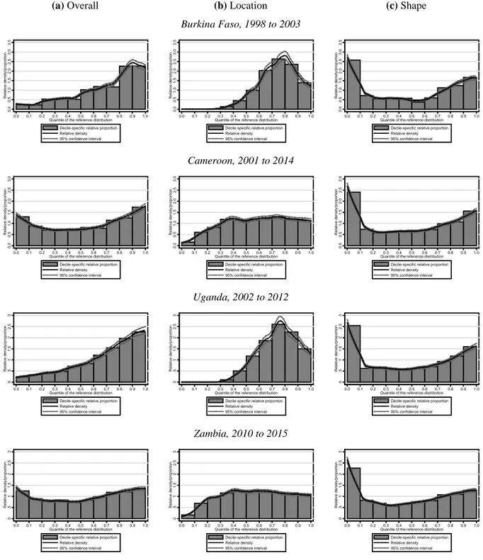
Figure 4 presents the overall distribution and the decomposition into location and shape for four countries selected from four different SSA macro regions, in order to give an idea of how regionally generalizable the identified distributional pattern may be. Burkina Faso is selected for West Africa, Cameroon for Central Africa, Uganda for East Africa and Zambia for Southern Africa. The left panel for each country represents the overall relative distribution, showing the fraction of households in the comparison year’s distribution that fall into each decile of the reference year’s distribution. The location effect is shown in the central panels of Figure 3. The panels on the right show the shape effect – that is, the relative distribution net of the median influence14.

Focusing on the shape effect, we find that all four countries display very similar distributional changes, notably a marked increase in concentration in the lower tail. Similar results are obtained by Clementi et al. (2019) using different time intervals. Relative to the reference period, the concentration of households in the lowest two deciles of each country increased by about 15 percentage points (+1.5 over 1) in Burkina Faso, Cameroon and Uganda and by 12 percentage points in Zambia. This increased concentration in the lower tails (also described as downgrading) occurred alongside a similar but smaller increase in concentration in the upper tails (upgrading). As shown in Figure 3, the two combined effects produce a quasi-U-shaped relative density. Over the period considered, in these 4 countries households became increasingly

14_{In the graphs, values above 1 indicate that, in relative terms, there are more households in that decile of the}

distribution at the end of the period than there were at the beginning, vice versa less than 1 means there are less, and equal to 1 means that things have not changed: 10 percent of households were in that decile at the beginning and 10 percent remained there.

(22)

22

concentrated in the tails of the distribution while the middle of the distribution tended to hollow out.

Figure 4: Relative distribution plots. Black dashed lines denote the relative density function obtained by fitting a local polynomial to the estimated relative data, while grey dotted lines indicate the 95% pointwise confidence limits based on the asymptotic normal approximation (Handcock and Morris, 1999, p. 144). The bars represent the decile breakdown of the relative distribution, showing the fraction of households in the comparison year’s population that fall into each decile of the reference year’s distribution.

(a) Overall (b) Location (c) Shape

Burkina Faso, 1998 to 2003 Cameroon, 2001 to 2014 Uganda, 2002 to 2012 Zambia, 2010 to 2015 0. 0 0. 5 1. 0 1. 5 2. 0 2. 5 3. 0 3. 5 Re lat iv e den s it y /pr op or tion 0.0 0.1 0.2 0.3 0.4 0.5 0.6 0.7 0.8 0.9 1.0 Quantile of the reference distribution

Decile-specific relative proportion Relative density 95% confidence interval 0. 0 0. 5 1. 0 1. 5 2. 0 2. 5 3. 0 3. 5 Re lat iv e den s it y /pr op or tion 0.0 0.1 0.2 0.3 0.4 0.5 0.6 0.7 0.8 0.9 1.0 Quantile of the reference distribution

Decile-specific relative proportion Relative density 95% confidence interval 0. 0 0. 5 1. 0 1. 5 2. 0 2. 5 3. 0 Re lat iv e den s it y /pr op or tion 0.0 0.1 0.2 0.3 0.4 0.5 0.6 0.7 0.8 0.9 1.0 Quantile of the reference distribution

Decile-specific relative proportion Relative density 95% confidence interval 0 .5 1 1. 5 2 2. 5 3 Re lat iv e den s it y /pr op or tion 0.0 0.1 0.2 0.3 0.4 0.5 0.6 0.7 0.8 0.9 1.0 Quantile of the reference distribution

Decile-specific relative proportion Relative density 95% confidence interval

(23)

23

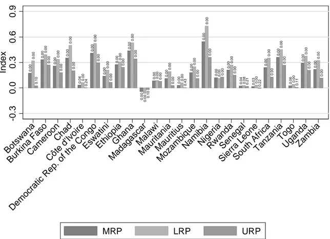
The performance of the remaining 20 countries can be summarized using the relative polarization indexes (Figure 5). Besides the 4 presented in detail above, other 18 countries show the same distributional change. All are undergoing an accentuated polarization process as evidenced by the positive and significant15 value of the MRP. Polarization is mainly driven by downgrading – reflecting a more accentuated concentration in the lower tail than in the upper. Supporting this, the LRP always exceeds the URP in magnitude and is always significant, whereas in 6 countries out of 16 the URP is not significantly different from 0. Madagascar and Nigeria are outliers to this otherwise homogenous pattern. Madagascar is the only country in the group analyzed where polarization decreases, while Nigeria is the only one where upgrading exceeds downgrading.

The picture that emerges from the analysis is of an increasing divide between the bottom 40 percent of SSA population and the rest. This bottom 40 percent coincides in most of the analyzed

15_{The null hypothesis of no change with respect to the reference distribution is tested for each index.} 16_{Botswana, Cote d’Ivoire, Mauritius, Senegal Sierra Leone and Togo.}

Figure 5: Relative polarization indices by country. The number close to each bar indicates the p-value for the null hypothesis that the index equals 0.

0. 0 0 0. 0 0 0. 0 0 0. 0 0 0. 0 4 0. 0 0 0. 0 0 0. 0 0 0. 0 0 0. 0 0 0. 0 0 0. 0 0 0. 0 0 0. 0 0 0. 0 0 0. 0 0 0. 0 0 0. 0 4 0. 0 3 0. 0 0 0. 0 0 0. 0 6 0. 0 0 0. 0 0 0. 0 0 0.0 0 0. 0 0 0. 0 0 0. 0 0 0. 0 0 0. 0 0 0. 0 0 0. 0 0 0. 0 0 0. 0 0 0. 0 0 0. 0 0 0. 0 0 0. 0 0 0. 0 0 0. 0 0 0. 0 8 0. 0 0 0. 0 0 0. 0 0 0. 0 0 0. 0 0 0. 0 0 0. 1 0 0. 0 0 0. 0 0 0. 0 0 0. 2 4 0. 0 0 0. 0 0 0. 0 0 0. 0 0 0. 1 0 0. 0 0 0. 0 0 0. 4 3 0. 0 0 0. 0 0 0. 0 0 0. 0 0 0. 2 1 0. 2 2 0. 0 0 0. 0 0 0. 1 1 0. 0 0 0. 0 0 -0. 3 0. 0 0. 3 0. 6 0. 9 Inde x Bot swa na Bur kina F aso Cam eroo n Chad Côt e d' Ivoi re Dem ocrat ic Re p. o f the Cong o Eswa tini Ethio pia Ghan a Mad aga scar Mal awi Mau ritani a Mau ritius Moz am bique Nam ibia Niger ia Rw and a Sen ega l Sie rra Leo ne Sout h Af rica Tanz aniaTogo Ugand a Zam bia MRP LRP URP

(24)

24

countries with those living below the poverty line and a certain amount of the so called vulnerable middle class – those at risk of poverty whose wellbeing is just above the poverty line but can easily fall below in the event of a negative shock. According to a recent report from the Ranzani and Paci (forthcoming) on structural transformation in SSA, this segment of the population remains trapped in a segment of the labor market characterized by low productivity, high seasonality and variability of incomes and whose living conditions have been only partially affected by the buoyant growth of the early 2000’s.

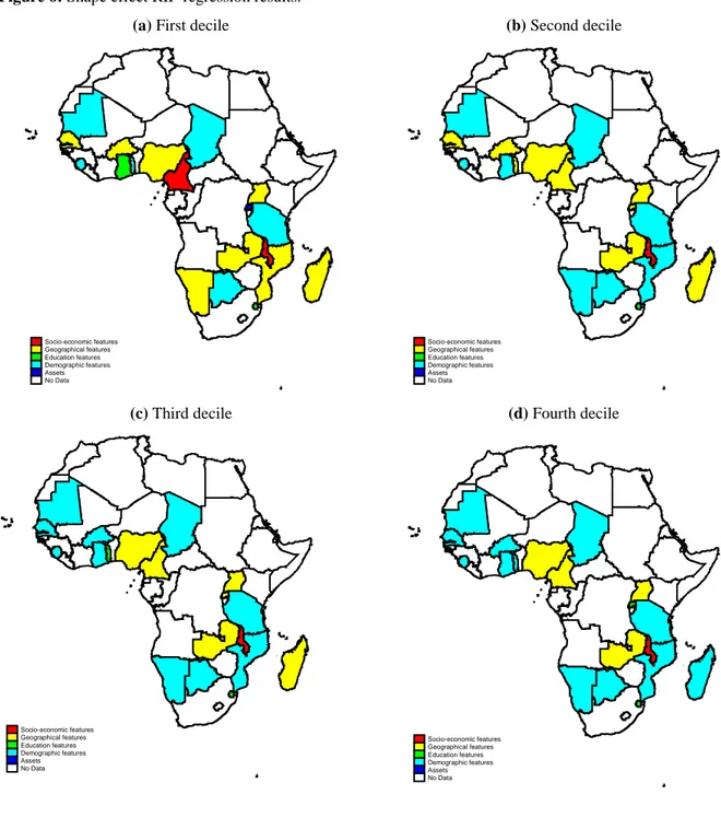
Having identified this downgrading (polarization in the lower tail) within the bottom 40 percent as the main distributional change in SSA over the last two decades, we proceed by analyzing the drivers of this process. For the sake of brevity, we present the outcome in map format. The full econometric and the Oaxaca-Blinder decomposition results by decile are all available upon request. We produced 4 maps (Figure 6 on the next page), one for each of the bottom four deciles, indicating the main driver of downgrading for every country.

Overall, results are rather homogenous in the countries analyzed. Drivers of downgrading are found to consist of two groups of variables: household characteristics and spatial/infrastructure covariates; both contributed to increase downgrading. Regarding demographic variables, this result confirms the urgency of addressing the demographic determinants of poverty risk: larger households with more dependents tend to be worse-off and benefit less from aggregate consumption growth. Likewise, the result on the spatial infrastructure variables (a group including access to basic services, infrastructure and place of residence) confirms that unequal access to infrastructure and regional developmental disparities within countries accentuate the divide between the poorest and the rest of the country.

In this regard, the Nigerian case is illustrative: Here, the spatial/infrastructure group of variables are consistently driving the downgrading process in all deciles considered. As pointed out by recent analysis on Nigeria (inter alia Clementi et al. 2017; World Bank 2016), this pattern of distributional change is driven by the widening of the north-south divide. Lower deciles are increasingly dominated by households residing in the North-West and in the conflict-stricken North-East, while at the top end of the distribution more households from the South tend to cluster. This process exacerbates the north-south divide that already characterized the country.

(25)

25

6 Discussion and conclusion

In the past two decades, SSA’s robust and sustained growth has been accompanied by poverty reduction rates which have lagged behind those of comparable developing countries. A common explanation for the non-inclusiveness of growth in the region is that the growth process which has predominated has been driven largely by growth in the primary sector. It has not been driven by, nor has led to, the kind of manufacturing-based structural transformation which has been

Figure 6: Shape effect RIF-regression results.

(a) First decile (b) Second decile

(c) Third decile (d) Fourth decile

Socio-economic features Geographical features Education features Demographic features Assets No Data Socio-economic features Geographical features Education features Demographic features Assets No Data Socio-economic features Geographical features Education features Demographic features Assets No Data Socio-economic features Geographical features Education features Demographic features Assets No Data

(26)

26

the historical hallmark of sustained poverty reduction and job creation in other developing countries (Rodrik, 2016, McMillan et al., 2014). The SSA growth pattern has remained characterized by the capture of resource rents by political and economic elites and is accompanied by the failure to develop secondary sectors which could lead to a more sustainable and equitable distribution of the fruits of growth.

In the context of this growth experience and in the face of SSA’s demonstrably low growth elasticity of poverty, it would be reasonable to expect inequality to have increased over this period (Bourguignon, 2004). However, when using standard inequality measures such as the Gini index, inequality trends in SSA do not display an unambiguous upward trend. Rather, inequality trends appear to have, over the past two decades, “bifurcated” (Odusola et al., 2017), with about half of the region’s countries experiencing declining inequality, and half experiencing increasing inequality. On average, there does not seem to have been any generalizable increase in inequality when measured using the Gini index.

However, in this paper we ask whether standard synthetic measures like the Gini might conceal as much as they reveal regarding distributional trends. We discuss how, in principle, this is possible if increasing inequality between top and bottom consumption groups is accompanied by decreasing inequality within these groups. For the purpose of linking distributional patterns to changes in poverty incidence, it is the clustering of households at the bottom of the distribution which is most relevant, and this clustering may be overlooked by standard measures. Specifically, we discuss and produce evidence on how a process of identification (decreasing within-group inequality) may compensate for alienation (increasing between-group inequality) when using standard inequality measures, and in this way misleadingly underestimate the severity of inegalitarian distributional trends. As long as alienation is more relevant to poverty reduction than identification, this feature of synthetic inequality measures makes them blunt tools for distributional analysis which aims to link to both growth and poverty reduction.

Decile dispersion ratios, which simply compare the consumption shares captured by top and bottom groups, are a class of commonly-used inequality measures that do not share these properties with synthetic measures. Because of this, they may be better suited to linking distributional analysis with an integrated analysis of growth and poverty reduction. Testing this hypothesis, we find that the D9/D1 ratio shows evidence of much more generalizable inequality increases across SSA than the Gini.

(27)

27

However intuitively appealing they may be, decile dispersion ratios remain crude measures. We propose that polarization analysis, using both synthetic indices as well as relative distribution analysis, may provide more complete and textured information about the nature of distributional changes which is sensitive to clustering of households at the top and the bottom of the consumption distribution – the most relevant changes for poverty reduction. Unlike standard synthetic inequality measures, in polarization analysis an increase in identification does not compensate for an increase in alienation. Within the family of polarization analysis, the relative distribution provides particularly rich information on the nature of the polarization process.

Applying these methods to comparable survey data from 24 SSA countries, we find that trends in polarization, unlike trends in inequality, have increased homogenously in SSA. In 23 out of 24 African countries where comparable data is available, distributional shifts over time were characterized by identification and alienation which led most strikingly to so called “downgrading” – that is, a clustering in the lower tail of the consumption distribution. Furthermore, for a subsample of these countries we also observe a significant but substantially smaller, “upgrading”, or a clustering in the upper tail of the consumption distribution. That is, we observe an increasing disparity between rich and poor, while at the same time decreased inequality within these groups. In this sense, polarization analysis using relative distribution methods represents a promising complement to standard inequality measures in that it is sensitive to certain distributional shifts that increase the divide between the poor and rich which standard inequality measures overlook.

Finally, we investigate the covariates of this polarization process. This investigation reveals that the drivers of polarization (and the clustering of households in the lower tail of the relative distribution in particular) are relatively similar across SSA: Demographic processes – in particular, high fertility rates among the poor – contribute to clustering in the lower tails of the consumption distribution, and as a consequence, to the degree of polarization. Urban/rural, regional variables and access to basic infrastructure are the most important drivers of downgrading in many countries in the first decile. However, these variables fade in importance the further one moves up along the distribution, with the notable exception of Nigeria - a country characterized by a very strong and increasing spatial divide.