Intelligent Systems for the Exploration of Structured and Complex Environments

(1)

(2)

(3)

Università Politecnica delle Marche Dottorato di Ricerca in Scienze dell’Ingegneria

Curriculum in Ingegneria dell’Informazione

Intelligent systems for the

exploration of structured and

complex environments

Ph.D. Dissertation of:

Nicolò Ciuccoli

Advisor:

Dott. Ing. David Scaradozzi

Curriculum Supervisor:

Prof. Francesco Piazza

(4)

(5)

Università Politecnica delle Marche Dottorato di Ricerca in Scienze dell’Ingegneria

Curriculum in Ingegneria dell’Informazione

Intelligent systems for the

exploration of structured and

complex environments

Ph.D. Dissertation of:

Nicolò Ciuccoli

Advisor:

Dott. Ing. David Scaradozzi

Curriculum Supervisor:

Prof. Francesco Piazza

(6)

Facoltà di Ingegneria

(7)

Abstract

Robotics is related with the development of robotic systems able to move know-ing the environment where they must act. The environments diversities have brought researchers developing indoor and outdoor robotic techniques and tech-nologies able to perceive movements and effects at the time arise. This work investigated possible design and implementation of mechatronic structures, able to work in industrial or complex unstructured environments.

As first aspect structured environment and needed sensors has been investi-gated. The work has been then expanded adding complexity to the aims and reducing the structures faced. During the work, three innovative mechatronic systems have been investigated. The first one regarded the highly structured industrial environment in which an intelligent and semi-autonomous station for testing domestic boilers during the production has been studied.

Considering a more challenging, not structured environment, where optical data need to be gathered with poses information, the author concentrated then on the underwater seabed reconstruction by means of photo cameras carried by divers. The most important challenge in the development of the designed platforms was the Unscented Kalman Filter (UKF) implementation to solve the navigation problem that fuses the data provided by an Ultra Short Base-line (USBL), an Inertial Measurement Unit (IMU) and a receiver for global positioning (GPS).

The work, after considering structured environment reconstruction by means of vision advanced techniques and after facing the situations without position-ing structures in the environment, closed with the study of a situation where the robot movement alter the pose but in a way that can be estimated and pre-vented. An innovative Backstepping controller with a non-linear disturbance observer (NDO) has been designed for the hybrid actuation of the underwa-ter robot under analysis reducing the oscillatory behavior introduced by the biomimetic propulsion.

Keywords: Object detection; image filtering; localization problem; Kalman

Filter; underwater applications

(8)

(9)

Sommario

L’attività di ricerca si è concentrata sullo studio, progettazione e realizzazione di sistemi di raccolta dati in ambienti strutturati e complessi. Si è iniziato stu-diando metodologie e sensori tipicamente utilizzati negli ambienti strutturati, in particolare quello industriale, per poi procedere sull’ambiente sottomarino (ambiente complesso).

Tre sistemi meccatronici innovativi sono stati realizzati. Partendo da un am-biente strutturato è stata sviluppata una stazione automatica per il collaudo dei boiler domestici installata al termine di una catena produttiva. In questo caso studio si è contribuito allo sviluppo e implementazione di tecniche di im-age processing per l’identificazione dei difetti. La macchina in questo momento lavora autonomamente presso un importante azienda italiana e nelle varie ses-sioni ha una percentuale di individuazione dei difetti superiore al 90%, con solo il 3% di falsi positivi: percentuali di gran lunga migliori a quelle ottenute dagli operatori esperti dell’azienda.

Considerando l’ambiente sottomarino è stato progettato e sviluppato un dis-positivo capace di collezionare dati per subacquei al fine di aiutare gli archeologi nell’esplorazione di siti archeologici e ricostruzione 3D. La sfida più importante nello sviluppo è stata implementare l’Unscented Kalman Filter (UKF) risol-vente il problema della localizzazione fondendo i dati forniti da Ultra Short Baseline (USBL), Unità di Misura Inerziale (IMU) e ricevitore GPS. Pros-eguendo nella tematica di raccolta dati in ambienti non strutturati è stato sviluppato un veicolo marino pesciforme autonomo a propulsione ibrida. È stato caratterizzato il sistema di visione del veicolo basato su action camera ed il sistema di controllo dell’orientamento. Il controllore realizzato (Back-stepping con osservatore non lineare del disturbo) ha permesso, tramite due motori brushless, la cancellazione del comportamento oscillatorio introdotto dalla propulsione biomimetica.

(10)

(11)

List of Figures

2.1. Red, Green, Blue (RGB) Cube2 _{. . . .} ₉

2.2. Hue, Saturation, Lightness (HSL) space3 _{. . . .} ₁₀

2.3. Edge model4 . . . 11

2.4. Edge Strength4_{. . . .} ₁₂

2.5. Edge Polarity4 . . . 12

2.6. Simple Edge Detection4 _{. . . .} ₁₃

2.7. Advanced Edge Detection4 _{. . . .} ₁₄

2.8. Example of Sobel operator . . . 14

2.9. Framework Test Robot . . . 15

2.10. Global Positioning System (GPS) receiver - Adafruit GPS Break-out5 . . . 24

2.11. GPS Trilateration6 _{. . . .} ₂₅

2.12. Ultra Short Baseline . . . 27

2.13. Short Baseline . . . 28

2.14. Long Baseline . . . 29

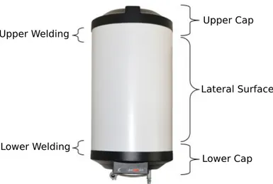
3.1. Boiler components . . . 36

3.2. Camera . . . 36

3.3. Lens . . . 37

3.4. The described defects . . . 38

3.5. The real test station . . . 39

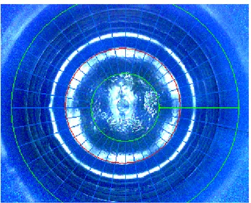
3.6. In red to circumference found . . . 40

3.7. Fall Glaze Filtering Process on 4.5 mm image . . . 41

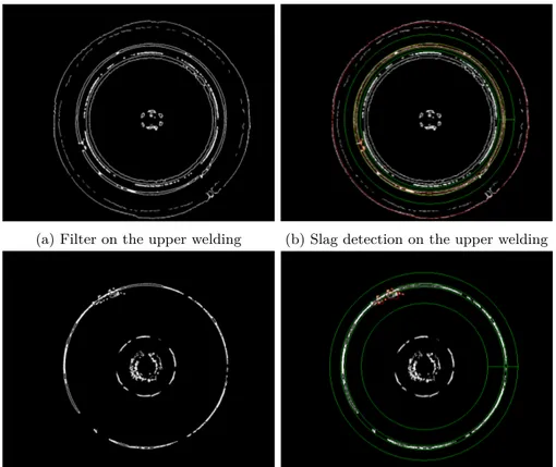
3.8. Slag filter on lower and upper welding . . . 42

4.1. Docking Station - Hardware Scheme . . . 47

4.2. Docking Station . . . 49

4.3. Mission Planner - Selection . . . 50

4.4. Mission Planner - 3D Map View . . . 50

4.5. Navigation app - Track view . . . 51

4.6. Navigation app - Camera view . . . 51

4.7. Estimated position by the Unscented Kalman Filter . . . 55

4.8. Estimated Position Error . . . 55

4.9. Depth and temperature during a mission . . . 56

4.10. 3D reconstruction . . . 57 xiii

(14)

4.11. Docking Station testing . . . 57

5.1. Brave Drawing Computer Aided Design (CAD) . . . 60

5.2. Brave . . . 61

5.3. Reference Frames of the Fish Robot . . . 62

5.4. Propulsive forces and torque decomposition . . . 64

5.5. Heading control diagram . . . 64

5.6. surge velocity at different thruster oscillation frequencies . . . . 68

5.7. Body rotation at different thruster oscillation frequencies . . . 68

5.8. Biomimetic Thrust at 1 Hz . . . 69

(15)

List of Tables

3.1. Camera parameters . . . 37

3.2. Defects during the comparison machine-operator . . . 43

3.3. Comparison results . . . 43

4.1. Nvidia Jetson TX1 characteristics . . . 46

4.2. IMU specifications . . . 48

B.1. Physical parameters . . . 77

B.2. Added mass and damping coefficients for a cylinder . . . 77

B.3. Propellers Parameters . . . 78

B.4. Biomimetic Thruster Parameters . . . 78

B.5. Controller and observer Parameters . . . 78

(16)

(17)

List of Abbreviations

AG-LGT Absence or Low Glaze Thickness. 35, 39, 43 AGV Automated Guided Vehicle. 6

AHRS Attitude and Heading Reference System. 17, 60 AUV Autonomous Underwater Vehicle. 27, 31, 59 CAD Computer Aided Design. xiv, 59, 60, 73 CCD Charge-Coupled Device. 7

CMOS Complementary Metal-Oxide Semiconductor. 7 DC Direct Current. 60

DG Discontinuous Galerkin. 63

DGPS Differential Global Positioning System. 26, 27 DOF Degrees Of Freedom. 5, 6, 20

DS Docking Station. 45–47, 51, 52

DSMS Docking Station Motion Software. 49, 51 DVL Doppler Velocity Log. 26, 27, 31, 73 ECEF Earth-Centered, Earth-Fixed. 54 EIF Extended Information Filter. 19, 30

EKF Extended Kalman Filter. 18, 19, 22, 27–31, 75 ENU East North Up. 52, 54

FOG Fiber Optic Gyroscope. 21, 22, 27, 73 GIBs GPS intelligent Buoys. 28

GNSS Global Navigation Satellite System. 22

(18)

GPS Global Positioning System. xiii, 19, 22–26, 47, 49, 52–54 GR Graniglia. 35, 39, 43

GRV Gaussian Random Variable. 18, 75 GS-FG Greasy Stain-Fall Glaze. 35, 39, 43 HSL Hue, Saturation, Lightness. xiii, 9, 10

IMU Inertial Measurement Unit. 17, 19–22, 27, 29, 46, 52, 53, 60, 73 INS Inertial Navigation Systems. 17, 19, 26, 27, 45

IoT Internet of Things. 47

KF Kalman Filter. 18, 19, 21, 27, 29, 75 LBL Long Baseline. 28–30

LSR Least Square Regression. 19, 20

MEMS Micro Electro-Mechanical Systems. 21, 22 MP Mission Planner. 49

NA Navigation App. 49

NAVSTAR GPS NAVigation by Satellite Timing And Ranging GPS. 22, 23 NDO Nonlinear Disturbance Observer. 64, 66, 67, 69

NN Neural Network. 33, 39 PF Particle Filter. 19, 22, 29–31 RGB Red, Green, Blue. xiii, 8–10 ROI Region of Interest. 11, 39 ROV Remote Operated Vehicle. 59 SBL Short Baseline. 28

SIFT Scale-Invariant Feature Trasform. 6

(19)

List of Abbreviations xix

SS Soldering Slag. 35, 39, 43 SSBL Super Short Baseline. 26

TCP Transmission Control Protocol. 51 ToF Time of Flight. 8, 17, 24–26, 28 UCH Underwater Cultural Heritage. 45 UDP User Datagram Protocol. 52

UKF Unscented Kalman Filter. 19, 22, 27, 45, 52, 54, 75 USBL Ultra Short Baseline. 26–28, 47, 49, 52–55, 71 WGS World Geodetic System. 26, 54

(20)

(21)

Chapter 1. Introduction

1.1. Operational Background

The development of intelligent robotic systems that explore every type of en-vironment by performing the inspection and documentation is a field of study with a constant increase in interest. Companies, Universities and research cen-tres are spreading more and more resources in the development of these robots. Anyway, in the past the robots had limited computing and sensory skills so they could perform only a limited number of tasks with little autonomy. Nowadays, robotic systems are equipped with a high number of highly efficient sensors that allow them to know their position in the world, their asset, to acquire and understand the environment state and to carry out all kinds of manipulations. The ability of a robot to move and perform its functions within its working space is becoming very important, so the robustness of the software and the sensors accuracy have become fundamental requirements in order that it can respond to a series of deterministic events. Based on this ability, the robots can be classified as:

• Not autonomous, which substitute the human in his activity because more efficient. Usually these types of robots work in structured environments and are driven by deterministic software or directly by humans.

• Autonomous, who carry out their activity in unstructured and complex environments, without the need for human intervention. Mobile robots are part of this category and the ability to navigate automatically within an environment is a non-prescriptive attribute.

The use of robots in activities such as visual inspection or quality control allows first of all to carry out these tasks in a rigorous and objective manner, compared to the man who in the past, and still today, has often done this activity not using the same evaluation criteria. In addition, the robotic sys-tems allow the performance of functions even in particular environments such as the submarine, the space, nuclear industries etc... obtaining very precise information, which for humans are difficult and dangerous.

(22)

1.2. Objective

The Ph.D research activity, explained in the present work, was born from the cooperation of the Università Politecnica delle Marche and the "BCB electric", an Italian company from the Marche region with strong know-how on automatic and intelligent mechatronic systems for quality assessment on production lines. The aim of the research was the study and development of mechatronic systems for the exploration of structured environments, such as the industrial one, or complexes like the underwater one. The systems have been equipped with more high-efficiency sensors, specifically vision, localization and inertial measurement units, combining and processing their information/measures in order to be used for inspection, documentation, mapping and reconstruction of the environment.

The main activities described in this thesis are:

• The study and development of image processing techniques. • The study and development of localization algorithms.

• The implementation and validation of these techniques on case studies in different environments.

The main environments taken into consideration are the highly structured in-dustrial one and the submarine one because they represent the two extreme cases in which a robot can operate, the first is completely known or easy to render, while in the latter there is no knowledge.

1.3. Thesis Overview

This dissertation starts with a review on sensors for structured and complex environment (chapter 2), in which, the first part explains in detail the sensors typically used in the industrial environment to carry out the inspection tasks, in particular the vision systems. The state of art continues by describing the image processing techniques used in the case of study in a structured environment. The second part of the chapter discusses the navigation problem and the sensors used for its solution up to describe those for the submarine environment and the data fusion algorithms.

The following chapters describe the case studies in the different environments that have been addressed. Chapter 3, "A Structured Environment Case study:

Video inspection test of domestic boilers", presents a case study where the

en-vironment is structured, a mechatronic system which automatically tests the domestic boilers, developed with the partnership of BCB electric s.r.l. After a brief discussion of the problem and the mechatronic system, the image filtering

(23)

1.3 – Thesis Overview 3 algorithms and the results obtained are described extensively. Chapter 4, "An

Unstructured Environment Case study: Underwater Documentation", presents

a platform developed within the European project Lab4Dive which helps marine archaeologists to explore archaeological sites. In detail the hardware architec-ture of the system and the localization algorithm has been described. Chapter 5, "System for exploration of complex environment" describes the case study for the complex environment, an innovative autonomous underwater vehicle with biomimetic/hybrid propulsion. The chapter begins by describing the robot, then moving on to the mathematical model and the heading control system.

(24)

(25)

Chapter 2. State of Art

In recent years robots are attracting increasing interest, due to their strong autonomy and ability to carry out relatively difficult tasks in different envi-ronments, especially autonomous vehicles that operate where humans can not. Based on the knowledge of the space in which the robot carries out its activi-ties, the environment can be classified as structured, when it is known how it is done, what will happen inside it, the possible agents that move, including their behaviour and the possible abnormal events that may occur. While an environment becomes unstructured when some of the previous hypotheses are missing, for example, the map, events or agents are not known until to turn into complex when the knowledge is minimal. A robot in order to acquire in-formation on the surrounding space needs tools that allow it to know its status and that of the environment. These instruments are called sensors that can then be defined, more precisely, as "devices that receive a stimulus and respond with an electrical signal" that can then be processed off-line or in real-time [25]. A very important classification for sensors for automation is that concerning the quantity to be measured:

• displacements, levels and proximity • force, deformation and tactile • flow

• vision systems • localization

A typical example of a robot moving in a structured environment by execut-ing its tasks is the manipulator. In [53] a 7 Degrees Of Freedom (DOF) ma-nipulator for industrial application was designed. This particular robot is able to know its state (position of the joints) and the objects presence to be taken by means of displacement and proximity sensors (encoder and photocells), or by means of a monocular camera [46]. Another important task performed by automatic machines in a structured environment is the inspection for quality 5

(26)

assessment purposes of components or for reasons of object detection that in the past was carried out by manual operators. In [69] a machine that carries out the blister packing inspection based on a vision system is presented. An example of object detection in a structured environment is illustrated in [96] in which video surveillance techniques has been implemented.

In recent years human-robot interaction in unstructured environments has become a research area with a steady increase in interest. In [68] the au-thors proposed a cooperation method between robots and human which per-mits agents to work together during navigation, combining their advantages in standalone performance, while in [93] asymmetric cooperation was tested be-tween a 6-DOF manipulator and human in an environment in which the robot can make mistakes and the human can help it.

In the industrial environment there are often Automated Guided Vehicle (AGV), robots that have the main function of transporting every kind of thing produced or logistics without the intervention of the human [72], but also used to carry out inspections [75]. These vehicles need to have specific sensors with respect to the robots described above because they have to solve the naviga-tion problem (described in detail in the secnaviga-tion 2.4). In an indoor environment (structured) an example of localization is provided by MA et all. [54] in which the vehicle is able to know its position by means of the geometric character-istics of the map, in [9] localization is performed by means of an algorithm called Scale-Invariant Feature Trasform (SIFT) which calculates the displace-ment based on how much the features extracted from an image has moved into the next. Another method for performing indoor localization is through the recognition of Landmark [51].

Localization task is the main problem to solve in complex environments like aerial [95] and [45], surface [20] and underwater [32], [73] in order for the robot to carry out its activities. This type of robot requires a sensor and a higher calculation capacity than the previous ones, having to process a greater amount of information.

2.1. Sensors for structured environment

Typical sensors adopted on robots that perform their tasks on structured envi-ronments are vision systems. It is a system composed of one or more cameras used for the reconstruction of the work environment map, for the objects iden-tification/detection and to interact with them.

The main components that characterize a vision system are the lenses and the frame grabber of the camera. The lenses are useful to change the direction of the light rays and to convey them in the desired way: when the light emitted by an object enters in a lens, its direction is modified according to Snell’s law.

(27)

2.1 – Sensors for structured environment 7 The position and size of the image that is created downstream of the lens depends on the focus, which indicates the plane or point where single rays forming a beam of distinct electromagnetic radiations coming from a point to infinity. Moreover, the type of lens is the element that characterizes the angle of view and the distortion of the acquired image.

The frame grabber is a lattice of photosensitive elements on a chip that produce a charge proportional to the brightness of the corresponding point of the scene, this charge is then converted into an image from the camera internal electronics. There are two different construction technologies:

• Charge-Coupled Device (CCD) in which the value of each pixel is treated independently of the others with the advantage of having a low consump-tion and a high reading speed. This technology causes a high level of independent noise for each pixel.

• Complementary Metal-Oxide Semiconductor (CMOS) in which the signal is transferred and processed for the entire photoelectric element, creating a high signal/noise ratio. The disadvantage is the higher consumption and the low reading speed.

Vision systems are widely used to test components at the end of production chains, for example in [69] a single monocular camera is used to inspect the blister packing inspection, while in [13] a system composed of 3 cameras to monitor the colour degradation of textile yarns and beverage.

For documentation purposes, vision systems are used in all kinds of environ-ments, as in [36],[63] and [38], in which helicopters were equipped with cameras to monitor the state of damage to cables, infrastructures or power lines, or on submarine vehicles [19] to monitor the status of the bridges or archaeological site.

In particular inspection applications where temperature monitoring is re-quired such as the health of electrical component [33], food inspection [86] or oil layer measurement [24] infrared cameras or thermo-cameras are used. The thermo-camera is a no contact device that detects infrared energy (heat) and converts it into an electronic signal, which is then processed to produce a thermal image and perform temperature calculations. The heat detected by a thermal imaging camera can be quantified or measured with extreme precision, allowing to monitor not only thermal performance, but also to identify and assess the relative severity of problems due to heat.

When the information of a 2D image is no longer sufficient, cameras com-posed of at least 2 lenses and 2 frame grabber are used. This device, called stereo camera, allows to simulate human binocular vision, and to obtain three-dimensional images or range measurement after a elaboration process [28].

(28)

Stereo cameras are used to check the quality of components. In [52] and [47] stereoviews is presented in order to verify the correctness of the solder on Circuit Board Printed, in particular the ball height and coplanarity, and the terminal lead are analysed. Other applications are the identification of faults in the sewer pipes [35] or factory defects in different types of products [34]. Stereo cameras is also the technology used to make 3D pictures and films.

A new technology widely used in the case of applications that need three-dimensional images are the Time of Flight (ToF) cameras that consist of a range imaging camera systems, which exploits the knowledge of the light speed and the answer time between it and the object for each pixel. Comparing it to the stereo vision these devices do not need texture and good lighting conditions to bring out the fundamental elements of the images. The main disadvantage is the low resolution and the maximum distance from the framed object of maximum 30 meters. Moreover, this type of sensor is very compact and suitable for obtaining 3D images with a high frame rate focusing the object only from a frontal point of view. In the industrial environment, these types of cameras have been used to solve the problem of bin-picking, i.e. a robot capable of recognizing objects, including their orientation, taking, placing and manipulating them in an orderly manner in his own work space. In [66] the authors present an algorithm for locating objects via ToF cameras. While in [58] is adopted to solve the bin-picking problem.

2.2. Image processing techniques

In this section all the image processing techniques used to identify faults in boiler enamelling will be reported1.

2.2.1. RGB colour model

The most usually representation of colour space is the RGB model, being re-lated to the physiology of the human eye. In fact, man has in the eye 3 types of conical photo-receptor cells with which he receives visual information divided into the three main chromatic components: red, green and blue, also known as

"additive primary colour". In this system, any shade it can be reproduced as

a combination of these primary colours. The RGB colour space can be viewed as a three-dimensional axis system, as shown 2.1 :

In this three-dimensional space, black represents the origin of the cube whereas the opposite end there from the white. The primary colours represent each side of the cube and take the value 0 in the origin ("No contribution") until to reach the value 1 at the opposite end ("totally saturated colour"). Each point inside

(29)

2.2 – Image processing techniques 9

Figure 2.1.: RGB Cube2

the cube represents a colour that can be represented by a tuple composed of 3 numbers (respectively the levels R G and B), in particular those located on the diagonal that cross the cube through Black (point [0,0,0]) and white (point [1,1,1]) are all different levels of grayscale colour, that is, in which the three primary components are matched. However, not all hardware and software use colour ranges between 0 and 1. The most commonly used ranges are 0-255 (also used for filtering in this thesis) and 0-65.535. Although the RGB space more closely reflects human vision and is easily used for the representation of a colour, there are some drawbacks. It may be difficult to select a particular colour only by interacting on the RGB levels without being able to choose ad-ditional features that will have to satisfy (to lighten a colour, for example, each of the 3 RGB components must be proportionally increased). Moreover, the RGB space can represent a quantity of colours lower than those visible.

2.2.2. HSL colour model

The HSL colour model has been developed to simplify the procedure for se-lecting a specific colour. In this space a colour is identified from this three characteristic: Hue, Saturation and Luminance. The Hue is defined as the degree of similarity of a colour to red, green, blue and yellow. Saturation rep-resents the level of hue purity. A vivid and ringing colour has a very high

2_{http://zone.ni.com/reference/en-XX/help/372916L-01/nivisionconcepts/color_}

(30)

value, while as the saturation decreases the colour becomes weaker and tends to Gray, so saturation is also commonly defined as the measure of the amount of Gray present in an image. The Luminance indicates the quantity of light present in the colour, if it appears light or dark and it is therefore related to the perception of the light emitted or reflected by an object. The brightness can then be interpreted as the amount of white or black present in an image. An image with a maximum brightness level is completely white while an image with a minimum brightness level is completely black. Compared to the RGB model in which the space is represented by a cube in the HSL model the colours are defined within a hexcone as shown in fig 2.2.

Figure 2.2.: HSL space3

The Hue values are shown on the circumference and they take values between 0◦and 360◦.At the value 0 there is the primary Red, at 120◦the primary Green is present while at 240◦ the primary Blue, and then returns to the primary

3_{http://zone.ni.com/reference/en-XX/help/372916L-01/nivisionconcepts/color_}

(31)

2.2 – Image processing techniques 11 Red at 360◦. Saturation and Luminance instead vary between 0 and 1. The saturation value 1 corresponds to a pure colour, while the luminance value 1 coincides to the white colour.

2.2.3. Edge detection methods

In the filtering phase it is essential to correctly identify the portion of the image to be analysed called Region of Interest (ROI). This region can be chosen as constant (appropriately defining the coordinates of this region), or it can be traced dynamically by exploiting the morphology of the image. For this purpose, different edge detection techniques can be used.

In a grayscale image an edge is defined as a substantial change in value between 2 adjacent pixels. This variation is generally sought along a one-dimensional profile that can take the form of a straight line, a perimeter of regular geometric figure or, more generally, a perimeter of a manually defined region. A software, which is looking for edges, examines the grayscale value of each pixel along the selected profile in order to identify significant or user-defined variations in intensity.

An edge is easily characterized by the model shown in the figure 2.3. As

Figure 2.3.: Edge model4

you can see for the correct identification of the border it is necessary to set the following parameters:

• Edge Strength. It indicates how much the grayscale value must vary between the background and the object for the edge to be identified. It is also called "edge contrast". Same object with different strength are showed in figure 2.4. The contrast of an edge may depend on several factors, including:

4_{http://zone.ni.com/reference/en-XX/help/372916L-01/nivisionconcepts/edge_}

(32)

– Light condition: if the general lighting of the framed scene is poor,

the edges of the bodies present in the image will be poorly defined and therefore the contrast will be low causing the visible effects in Fig. 2.4.

Figure 2.4.: Edge Strength4

– Bodies with different grayscale characteristics: if there are objects

illuminated differently in the scene, the edge of the less illuminated objects will be low.

• Edge Length, it defines the maximum distance (segment length) within the analysis profile in which the pixel value must vary. In other words, it indicates the speed of colour variation. So It is necessary to define a greater length to identify the edges characterized by a gradual transition between the background and the object.

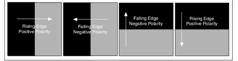
• Edge Polarity, it indicates whether the grayscale value is increasing (rising edge) or is decreasing (falling edge). It is therefore necessary to define a direction along which to analyse the edge as shown in Fig. 2.5

Figure 2.5.: Edge Polarity4

• Edge Position: it indicates the x, y coordinates in which to place the border point inside an image once identified, as shown in Fig. 2.3 Different edge detection techniques have been developed, the most commonly used in this thesis are the following:

• Simple Edge Detection. This technique consists in analysing pixel by pixel, all the points along the selected profile.

(33)

2.2 – Image processing techniques 13 In the first point where the contrast value between two pixels exceeds the set threshold (Edge Strength) added to a certain hysteresis value, a rising edge is detected. The hysteresis value is then used to define different Edge Strength thresholds for both sides. Once a rising edge has been identified, the method searches for a falling edge, as shown in Fig 2.6. This process is repeated for all the pixels along the profile to be

Figure 2.6.: Simple Edge Detection4

analysed. This technique provides excellent results for images that are not subject to noise, and therefore in which the object’s colour quickly deviates from the rest of the image.

• Advanced Edge Detection. This technique differs from the previous one by the fact that the intensity value along the profile is calculated within a defined spatial window, allowing to limit the error caused by the noise in simple edge detection procedure. Once the punctual average is calculated for each pixel along the profile, as for the previous technique this value is compared with the following ones and checked with the contrast threshold (Edge Strength). The spatial window must be chosen based on the noise, a high-noisy image requires a larger spatial window than a low-noisy image. The advance edge detection is showed in fig 2.7. Identified all the probable edge is selected and labelled the one with the most contrast as Start Edge Location (SEL). In order to find the End Edge Location (EEL) point the steepness parameters is added to the Start Edge Location. The Edge location is identified as the first point between the Start Edge and End Edge location such that:

Ip− ISE>= (ISE− IEE)/2 (2.1)

where Ip, ISE, IEE are respectively the intensity of the point in exam,

(34)

Figure 2.7.: Advanced Edge Detection4

• Sobel Operator [76]. It is a differential operator, which calculates an approximate value of the gradient of a function that represents the bright-ness of the image. The algorithm consists in the convolution of the image with an integer valued filter of dimensions 3x3, applied both directions (horizontal and vertical) and it is therefore "economic" in terms of re-quired computational power. After applying this operator to an image the gradient norm corresponds to each pixel. On the other hand, the gradient precision is relatively low, especially when the image is subject to rapid and frequent variations. The operator calculates the brightness

(a) Original image (b) Sobel Operator Figure 2.8.: Example of Sobel operator

gradient of the image at each point, finding the direction along which there is the highest possible increase from light to dark, and the rate at which change occurs along this direction. The result obtained provides a measure of how "abruptly" or "gradually" the image changes at that point, and therefore of the probability that that part of the image represents a contour, and also provides an indication of the probable orientation of that contour. In mathematical terms, the gradient of a function of

(35)

2.3 – Framework Design 15 two variables (here the image brightness function) is at each point of the image a two-dimensional vector whose components are the derivatives of the brightness value in the horizontal and vertical direction. This means that in the areas of the image where the brightness is constant the Sobel operator has zero value, while in the points on the edges it is a vector oriented through the contour, which points in the direction in which it goes from dark values to clear values.

2.3. Framework Design

Mechatronic systems equipped with vision systems can perform very different tasks, sometimes they are machines specifically designed for the execution of a unique activities of their kind. However, the documentation systems, having part of the common sensors, in particular the cameras, perform some generally common functions such as trying to understand the environment state from sensors, the acquisition and processing of images, the search for objects within the image, the fusion of information and then make decisions based on the results of these elaborations. This section presents a general framework, which describes the main activities of an exploration/documentation system. Figure 2.9 shows the framework block scheme.

Environment Robotic System Camera 1 Camera 2 Camera n Sensor 1 Sensor 2 Sensor n Decision Making Robot Sensors Sensor Acquisition Images Acquisition Images Processing Vision System Environment Status

Figure 2.9.: Framework Test Robot

The environment can be of any type (stuctured, unscructerd or complex) and it is the place where the robot moves to accomplish its task. The environ-ment knowledge is a fundaenviron-mental task, so the mechatronic system needs to be equipped with a set of sensors whose characteristics are adequate to measure his state.

Sensors can be of various types: proprioceptive or exteroceptive, displace-ment sensors, localization and/or vision systems. The acquisition process of both the images and the measurement coming from the other sensors is funda-mental because quality information allows better performance of the apparatus.

(36)

The images processing block contains all the image elaboration algorithms for the reconstruction of the environment or for object detection that can be performed on-line, and then fuse this information with the other sensors mea-surement to obtain the status of the environment and robot.

The last block, called "Decision Making", consists of the intelligent part of the machine, that is, the module that decides which actions must follow and then continue with its own tasks.

2.4. Navigation Problem

A mobile robot called to complete a task in an unknown environment without the aid of man it is necessary for it to answer the following questions [26]:

• How do I know where I am? • How do I know where I must go?

• How do I know how to go to the destination point?

The first problem is defined as a problem of localization: the robot must be able to estimate its position from a starting point or inside a map (known in advance or dynamically constructed as a result of robot movements). The sec-ond problem is defined as target identifying: the robot, known as the starting point, must be able to define the next point to move; the intermediate points between the departure and arrival points are called way-points. The third one is called the problem of defining the trajectory: the robot, known the starting point and the arrival point, must be able to establish the path to follow, re-specting suitable specifications (e.g.: avoiding possible obstacles on the route). These three problems together contribute to the so-called "Navigation

Prob-lem". To achieve this goal, different sensors and techniques have been adopted

in literature. There are two possible approaches to localization:

• Dead Reckoning, the robot estimates his position based on the path it has made. The starting position is known, the robot deduces the current location by integrating the path travelled, it is also necessary to know the direction of the motion (orientation), the space travelled, the speed, the acceleration, the time, etc... Moreover the errors accumulate over time. • Map-based Positioning, the robot measures its position with respect to

reference points. It can be realized by providing a map of the environment in which the robot must operate, in this case the obtained localization has a high accuracy but the constraint that the robot can not leave the known area; or providing the tools to build a map autonomously but getting less

(37)

2.4 – Navigation Problem 17 accuracy map. Positioning in maps built by the robot during navigation is called Simultaneous Localization and Mapping (SLAM) Both approaches require different types of sensors. Especially for the first approach it is necessary to have a sensorial system able to perceive the move-ment of an object with respect to the surrounding environmove-ment because in the field of robotics most of the control algorithms are designed on this sensorial data, therefore their availability and reliability is a fundamental requirement.

An Inertial Navigation Systems (INS) is a system that can capture the ob-ject’s navigation information (linear and angular positions and velocities) in its reference space and transform it into the "absolute" reference space. In many applications it is not necessary to know the complete navigation information, but it is sufficient to know only the inertial measurements (linear acceleration and angular velocity), in these cases we speak of Inertial Measurement Unit (IMU). In other applications it is sufficient to have only the attitude measure-ments (angular positions) and, therefore, it is possible to combine a IMU with a processor for the resolution of the alignment equations, in this case we are talk-ing about Attitude and Headtalk-ing Reference System (AHRS). An INS consists of the following sub-systems:

• IMU.

• a microprocessor for the calculation of the structure. These two elements make up a AHRS.

• Navigation Aids, a set of sensors that provide aid measures that, com-bined with the previous ones and inserted into data fusion algorithms, allow to obtain a better estimate of the motion parameters.

Among the most widespread navigation aids in mobile robotics it is possible to mention:

• radio transmissions form earth base station,the receiver is equipped with an antenna that allows to receive the position of the ground station and calculate its position by means of triangulation;

• sonar, the receiver is equipped with an ultrasound system based on ToF able to estimate its height relative to the ground or its position with respect to a known map;

• laser range finder, as for the previous one, a system based on ToF but with superior performance;

• vision system, through the images provided by a camera it is possible to obtain the position or the movement made.

(38)

• magnetometer, the receiver is equipped with a sensor that, by measuring the earth’s magnetic field, can provide an estimate of the orientation in static conditions;

• GPS receiver, the absolute position estimate in external environments is obtained by means of a receiver equipped with an antenna.

On this system a recursive algorithm is implemented that estimates the state of the system xk composed of location and orientation. This algorithm calculates

at each instant time:

P (xk|u0:k, y0:k, x0) (2.2)

where u0:k and y0:k are respectively the histories of control inputs and sensors

measurements, and x0 the initial state. This formula indicates that the

pos-terior probability density of the state vehicle is calculated starting from the knowledge of the previous inputs, measurements, and of the initial conditions. Nonlinear discrete-time model including process n(k) and measurement v(k) noise is used to represent the state propagation.

{

x(k + 1) = f (x(k), u(k), n(k))

y(k) = h(x(k), v(k)) (2.3)

Typically, Bayes’ filter approximation is used to estimate the state. It is divided into two steps, prediction [85]:

The main techniques used are [62]:

• Kalman Filter (KF). It is an algorithm that estimates the state of a system starting from the measurements and from the model, which for hypothesis must be linear. Furthermore, the state distribution is approximated to a Gaussian Random Variable (GRV), so both the model uncertainty and the measurement noise are modelled as white Gaussian noise with a zero average which enter linearly in the process.

• Extended Kalman Filter (EKF). It is an extension of the KF to nonlinear processes, where the model is linearized at the work point at any time instant. Also in this case it is assumed that the noise enters

(39)

2.4 – Navigation Problem 19 linearly both in the state and output equation. The estimate obtained is good if there are small non-linearities in the model.

• Unscented Kalman Filter (UKF). Other KF for nonlinear systems. It reduces errors due to the linearization of the EKF propagating sigma points in the process equations. It improves estimation by increasing computational complexity. In the appendix A this algorithm is described in detail.

• Extended Information Filter (EIF). [84] Information Filter is an al-gorithm based on the same hypotheses of the KF, the main difference is that the state and covariance estimates are parametrized by the in-formation vector and matrix. This technique allows to process multiple measurements in a single moment of time by summing their information matrices and vectors, speeding up the update times. The main disad-vantage is that it takes time to recover the mean and covariance of the state.

• Particle Filter (PF). This category includes a set of sequential Monte Carlo algorithms to compute posteriors the state distribution in partially observable Markov processes. The common idea of these filters is that the distribution is represented by a set of random state samples called

"parti-cles". The main advantage is that it can be applied almost to all processes

that can be modelled as a Markov Chain. Performances deteriorate as the space dimension increases.

• Least Square Regression (LSR). The update equation can be formu-lated as a least squares problem which can be solved analytically. This technique has the advantage of taking into account all the past states, allowing to optimize the whole trajectory as well as being widely used in SLAM.

These filters are used in both aero, land, surface and submarine vehicles. Of course in submarines as explained below it is necessary to introduce sensors specifically designed for the marine environment, both in Dead Reckoning and Map-Positioned Based localization. For example, an adaptive version of KF was used in [94], [29], [31] for the realization of INS for vehicles composed of GPS/IMU which returns the orientation and position as latitude, longitude and altitude. Instead, in [95], [45] the EKF was used, in particular in [45] the vehicle mathematical model was exploited obtaining greater precision than [95] which used the uniformly accelerated motion model. UKF has been used in [1] where the problem of locating a submarine vehicle has been addressed. There are examples of EIF both in aerial [88], [87] and underwater environment [20]. PF is another technique widely used in systems composed of IMU/GPS [43].

(40)

In addition, in [79] and [90] the data provided by a vision system are merged together with the position, acceleration and speed data. LSR can be found in [18] in which the authors estimate the position of a mini mobile robot inside an indoor environment.

While for the SLAM only some Navigation AIDS are typical sensors such as laser range finder, ultrasonic sensors and Visions systems that allow to iden-tify landmarks, meaning relevant objects, salient points, within the map built on-line or known a priori. In SLAM the algorithms are always in the form prediction-update, in which at every instant the probability m of the environ-ment map is also estimated, then the formula 2.2 becomes [85]:

P (xk, m|u0:k, y0:k, x0) (2.6)

2.4.1. Inertial Measurement Unit

IMU is a unit of sensors composed of accelerometers and gyroscopes that pro-vide the measurement of linear accelerations and angular velocities. The classic configuration of these sensors is called "strapdown", the inside of which the sen-sitive axes of inertial sensors (gyroscopes and accelerometers) are mutually orthogonal in a Cartesian reference system. A unit in strapdown configuration can contain:

• 3 single-axis gyroscopes and 3 single-axis accelerometers; • 2 two-axis gyroscopes and 3 single-axis accelerators.

The sensors are rigidly connected to the housing of the unit, which is in turn installed on the object whose motion is to be measured, using an anti-vibration system.

Another type of configuration is the "skewed" which provides for the place-ment of gyroscopes and accelerometers on a tilted cone at a certain angle to the vehicle. The main advantage of this configuration is that it guarantees a certain fault tolerance because there are redundant elements. It is also able to measure angular velocities outside the measuring range, by scaling the actual velocity with the inclination angle of the sensors. With the same performance to be achieved it is good to know that the skewed configuration introduces more errors than the strapdown, therefore, requires higher quality gyroscopes and the exact knowledge of the inclination angle, otherwise it is subject to strong errors due to misalignment.

In the modern IMU the magnetometer has been introduced, a device able to provide a measure of the three dimensions earth’s magnetic field. In this case we talk about IMU at 9 DOF compared to 6 of that made up of only accelerometers and gyroscopes. The magnetometers are used as electronic compasses able to

(41)

2.4 – Navigation Problem 21 provide the orientation of the sensor with respect to the Earth’s magnetic north. This sensor requires a calibration after each installation because every metallic device has its own magnetic field that is not distinguishable from the terrestrial one.

There are different types of construction based on the physical principle of both accelerometers (mechanical, capacitive, piezoelectric, piezoresistive, heated gas) and gyroscopes (Mechanical, Laser, Fiber optic) [25], a widely used technology is Micro Electro-Mechanical Systems (MEMS) that allows the realization of IMU of reduced dimensions, and being suitable for the production of large volumes are very economical. These devices have the main advantage of being very robust to shock and vibration, but have a high sensitivity to tem-perature variations and in the gyroscope there is the output drift that must be eliminated by calibration. For this reason, Fiber Optic Gyroscope (FOG) are used in vehicles, which, even if very expensive, make it possible to obtain very small estimation errors after hours of use.

A IMU is subject to the following sources of error:

• Bias, It is defined as an independent and uncorrelated additive value (of acceleration or angular velocity) that manifests itself in IMU. Generally the 90% of the bias occurs at power-up, while the remaining 10% is due to temperature effects.

• The imperfect knowledge of the scale factor (ratio between the variation of the measurand and the variation of the measurement) implies a deviation between the sensor output and the value of the measurand, which however can be compensated by the internal filter to the IMU.

• No orthogonality. The strapdown configuration requires orthogonality between the sensitive axes of the sensors: if this orthogonality is lost (un-certainty in the construction of the sensor) then an error occurs. Usually this error is corrected during calibration by a series of tests that provides orthogonal rotations.

• Noise. It derives from electrical and mechanical instabilities and it has a Gaussian distribution at rest, which however can vary during the move-ment of the unit: it is possible to limit (but not to cancel) the filtering effects.

An evaluation of the MEMS accelerators was performed in [61], in which the distance traveled was obtained by double integration inside a KF which limited the effect of the noise. Random bias drift due to temperature variations also proves a significant increase in the error, requiring subsequent calibration by means of other external measures. The final experiment shows that this type of sensor can be a solution for short distance measurements.

(42)

Similar analysis was performed for MEMS gyroscopes in [92], in which angle output deviation was evaluated, caused by both the magnetostatic and elec-trostatic field. The deviation results to be much greater for the magnetostatic. Other very important properties to analyse in order to understand the work-ing performance [27] are the vibrational ones (rivwork-ing resonant frequency and detection resonant frequency).

In [16] and [67] several IMU have been compared. A first static analysis allowed to evaluate the noise, the stability of the bias even in the presence of magnetic fields. A second kinematic analysis integrating the unit with a GPS receiver was made to verify the validity of this solution for the mobile mapping application or for the direct photogrammetry on air vehicles. As expected, the unit equipped with FOG turned out to be the one with a lower drift and error after prolonged use.

The magnetometer has been used in various fields of application. In [80] a study was presented on the measurements coming from the magnetome-ters installed on the Android-based platform, observing the phenomenon of interference due to external devices, and developing a calibration algorithm to compensate them. In [70] the possibility of using the MEMS magnetometers for the determination of the spacecraft’s attitude is assessed, finding sufficient requisites in some of them. In [83] the magnetometer is used to estimate ori-entation as well as its rate of turn, offering different solutions with different computational complexity and precision, in order of precision and complexity: PF, EKF and UKF.

A new constructive solution was presented in [57] and [49] in which the performances of the MEMS magnetometers based on the physical principle of Lorentz force were improved in terms of sensitivity to external interferences, resolution and noise.

2.4.2. Global Positioning System

GPS is a system able to provide the position of a point on earth starting from the calculation of the distance from some known points in space (satel-lites). North American origin system, called NAVigation by Satellite Timing And Ranging GPS (NAVSTAR GPS), is the most common , but in reality there are others: the GLONASS (Russian), the GALILEO (European) and the BEIDOU/COMPASS system (Chinese) are still being tested. In the common language the NAVSTAR GPS system is usually abbreviated with GPS, a new term has been coined to indicate a "generic" global positioning system, that is Global Navigation Satellite System (GNSS) which indicates the 4 existing. The NAVSTAR GPS system consists of three basic segments:

(43)

2.4 – Navigation Problem 23 • the user segment (receivers),

• the control segment (stations).

The space segment consists of 24 operational satellites (plus 8 in reserve) that orbit at around 20000 km in height in 6 flat orbits (4 satellites for each orbit) with an inclination of 55◦ with respect to the equator and a revolution period of about 12 hours. Each satellite brings on board:

• a high precision atomic clock; • a control computer

• a radio system for L-band transmissions (from the satellite to the control and user segment) and S-band (from the station to update the almanac and ephemeris);

• a rockets system for attitude control.

The control segment includes 12 ground control stations with the following functions:

• keep the atomic clocks of the satellites in sync; • monitor the orbits of the satellites;

• monitor the status of the satellites (faults, malfunctions).

All the stations are automatic and continuously receive the signals emitted by all the satellites, their position is known with high precision and the recep-tion of the signals takes place using very sophisticated receivers, equipped with watches of the same type as those carried on board the satellites. Each station is equipped with meteorological instruments to evaluate the effect of the at-mosphere on the signals received and make the appropriate corrections. Four stations are able to send messages to satellites, and in detail these messages contain:

• the updated values of the ephemerids and almanac ; • the clock correction parameters;

• some data on the model of the atmosphere.

The user segment of the NAVSTAR GPS system consists of end users, whether civil or military, equipped with a receiving device consisting of:

(44)

• a clock (digital quartz, therefore not as precise as the one installed on board the satellites);

• a unit of calculation; • a management software.

The cost of GPS devices for the end user is very variable and depends mainly on the accuracy achievable with the same (from 10 m for devices without any type of correction up to 3 m for the most sophisticated devices). The signal

Figure 2.10.: GPS receiver - Adafruit GPS Breakout5

sent by the satellites consists of two carriers (L1 = 1575.42 MHz and L2 = 1227.60 MHz), two or more digital codes (Coarse Acquisition code or C/A on L1 and P-code on both L1 and L2), and a navigation message. Civilians have access to only C / A code on L1: the P code is encrypted with an unknown code, resulting in a signal used only for military purposes and called "antispoof-ing": the use of this code allows a very precise estimate. The new satellites recently introduced into orbit transmit two additional codes (L2 CM - Civilian Moderate and L2 CL-Civilian Long): these signals are useful for minimizing errors due to the effects of the atmosphere. The navigation signal contains in-formation about the almanac, ephemeris, clock correction, satellite health and atmospheric compensation factors: it is added to both the C/A and P signals. The C/A and P codes contain the satellite identity and the synchronization information: they are then modulated by the L1 carrier (both the C/A code and the P) and by the L2 carrier (P code only).

The principle of operation at the base of the position calculation by GPS is based on trilateration: the position of an object on the earth’s surface is deter-mined starting from the ToF of the signals sent by two satellites to the same receiver. The product between the ToF and the speed of light in a vacuum allows to estimate the distance between the single satellite and the receiver (the radius of the circle that has the satellite centre and the circumference

5_{https://www.distrelec.de/en/mtk3339-gps-breakout-adafruit-746-gps-breakout/p/}

(45)

2.4 – Navigation Problem 25 passing through point, see fig. 2.11), and the intersection of the two circumfer-ences makes it possible to identify the point on the earth’s surface. Since the distance calculation takes place indirectly starting from ToF, we are talking about pseudo-distance, indicating that it depends on time: a small error in the measure of time, in fact, can lead to a big error in position. If the measurement of a third satellite is used, however, it is possible to correct the time offset and identify a curved region within which to position the receiver. Since all GPS measurements are performed for three-dimensional localization, the signals of at least 4 satellites are required to obtain latitude, longitude and altitude.

Figure 2.11.: GPS Trilateration6

The receiver reproduces the C/A code of each satellite, varies its delay and calculates the correlation with the received C/A signal. The delay that maxi-mizes the correlation, multiplied by the speed of light in the vacuum, returns the pseudo-distance between the satellite and the receiver (three pseudo-distances for the trilateration and one for the compensation of the offset of the receiver). The satellite positions are known because each satellite sends the ephemeris in-formation as part of the navigation message. The receiver then solves a system of 4 equations in 4 unknowns:

Di=

√

(x − xi)2+ (y − yi)2+ (z − zi)2− cδi=1,..,4 (2.7)

where

If measurements from more than 4 satellites are available then it is possible to apply a least squares algorithm to obtain an optimal estimate of the position of the receiver.

(46)

One way to improve the receiver position estimation is to correct it with a term provided by a reference station whose position is known a priori. This system is called Differential Global Positioning System (DGPS) which allows to reach uncertainties of the order of 1 meter. A similar principle is used by kinematics satellite navigation (Real Time Kinematics GPS - RTK GPS), which takes into account the carrier instead of the modulated signal which is at a much higher frequency, reaching an accuracy of less than 10 centimetres.

2.5. Sensors for underwater environment

The navigating problem in the water is an even more difficult challenge. The difficulties of the environment due to the lack of light, the presence of sea cur-rents, the turbidity and the high attenuation coefficient of water add complexity to the estimation algorithms and make several sensors, that have an excellent behaviour in the air, unusable, such as GPS or radio transmission sensors INS use a set of measurements from sensors specifically designed for the submarine environment.

The Doppler Velocity Log (DVL) is used to measure the velocity in surge, sway and heave directions and the distance from the seabed. It transmits a series of acoustic beams and by measuring the Doppler shifted returns calculates these speeds. For the measurement of each velocity the device must emit a beam so usually these devices emit at least 4 beams. They have a good precision, in fact the standard deviation of the measurements is between 0.3 and 0.8 cm/s. Underwater depth can be measured with a barometer or pressure sensor. The precision that can be reacted with this sensor is of the order of the centimetre. The problem of localization is solved through acoustic navigation techniques by means of devices that measure the ToF of acoustic signals.

Ultra Short Baseline (USBL) is one of the most common method, also some-times called Super Short Baseline (SSBL). It involves two acoustic devices, a transceiver mounted on a surface vehicle or a buoy, called "head transceiver" and a transponder on the underwater vehicle. The term "baseline" indicates the distance between the transducers in the transceiver head, which are usually at least three spaced about 10 centimetres. The communication between the 2 devices starts from the head that sends an acoustic impulse, the submarine transponder detects it and replicates it with its acoustic impulse, in turn identi-fied by the transceiver. The range is measured by the head multiplying the time between the emitted and received pulse (ToF) with the sound speed in water. Position is subsequently calculated starting from this distance and from the the received pulse angle. The algorithm called "phase-differencing" is used to calculate the direction of the pulse emitted by the transponder. Furthermore, if the head knows its position in World Geodetic System (WGS) coordinates

(47)

2.5 – Sensors for underwater environment 27 it is able to calculate the position in the same coordinates. Fig. 2.12 shows the operation of USBL. With this method it is possible to locate vehicles at a maximum distance of 200 meters from the head.

In [71] in order to map and inspect the hydro dams an Autonomous Under-water Vehicle (AUV) equipped with IMU, FOG, DVL and a USBL has been developed. The head mounted on a buoy equipped with a DGPS allowed to improve the accuracy of the estimate obtained. Twp different EKF have been implemented: one to estimate the position of the vehicle and the other to trace and follow the dam wall identified by a mechanical scanning imaging sonar. For missions of this type the USBL turns out to be very adapted because the areas to be covered are reduced. A precision improvement was obtained in [1] where in a vehicle with the same sensors the UKF was implemented. Furthermore, an increase in the robustness of the INS was obtained by using the vehicle model in [1] and [32], allowing to examine many scenarios, including sensor removal or dropouts.

In [4], a sensor-based integrated guidance and control law is designed to pilot an underactuated AUV by USBL positioning system, in which the head transponder is installed on a known fixed position.

In [91], two algorithms for the tracking based on USBL measurements were introduced. The first method uses a simple KF which keeps the drift error limited, while in the second it is also considered the systematic error on the speed of sound, and, since the model is non-linear, EKF was used as a fusion technique.

(48)

A second technique is Short Baseline (SBL). It is very similar to the previous one, it differs in the fact that on the vehicle of surfaces there are two transceivers positioned aft and bow of the ship. (fig. 2.13). This system becomes more precise as the baseline increases, thus increasing the size of the boat. When

Figure 2.13.: Short Baseline

the accuracy and reliability requests exceed the capacity of USBL and SBL Long Baseline (LBL) or GPS intelligent Buoys (GIBs) are used, which consists in placing several transceivers at least three on the bottom for the first or on buoys for the second and calculate the position by triangulation. Figure 2.14 shows an example of LBL. The main limits of LBL are the cost and set-up times, as well as to have greater precision and the position in absolute coordinates requires the exact knowledge of the transponders position.

A high-precision LBL system was presented in [48] in which 3 transponders were positioned within a range of 700 meters, achieving an accuracy of ±30 centimetres. In order to achieve this result the position of the transponders was measured with a precision of ±8 centimetres by measuring the two-way ToF between transponders and a shipboard transducer with a resolution of the microsecond. While in [6] GIBs is developed, system composed of three transponders hanging on different buoys with the limit of 500 meters maximum depth. This system has been developed to cover very large areas, tens of kilometres with maximum errors in the order of 2% of the range.

In [12] a Bayesian Near Real Time estimation algorithm is presented for navigation with LBL transceivers. This approach combines a traditional EKF used between the LBL measurement and optimal Bayesian trajectory when the

(49)

2.5 – Sensors for underwater environment 29 point is received from the positioning system.

Figure 2.14.: Long Baseline

Modern technology has made it possible to localize through individual transceiver positioned on the bottom, this method is called "Single Fixed Beacon", and through acoustic modems positioned on autonomous non stationary vehicles.

An example of navigation with a single beacon is [50] where this technique, called virtual LBL, was simulated using real data. In [50] the impact of this system on the vehicle’s observability has been investigated, demonstrating that for some types of path, in particular long distance lines, the position error diverges. In order to solve this issue the vehicle must travel long distances in the tangential direction to the circular beams emanating from the single transponder.

The same problem has been addressed in [3] for a vehicle equipped only by a IMU, in which first the necessary and sufficient conditions for observability were analysed in order to control the path, and then a KF was implemented to estimate the position.

In [23] the homing problem, that is, the task to return the vehicle to the starting position (origin) fixed on the surface, has been resolved through the Single beacon navigation. Both the PF and the EKF have been designed and compared in terms of performance. To obtain good results the PF has risked a high number of particles while EKF requires assumptions on the type of noise, therefore the best performances have been obtained through a mixed solution. All these methods have a latency and a low rate in the calculation of the position, so prediction of the state estimation algorithms is provided by the

(50)

measurements from the dead reckoning sensors until the acoustic measurement that provides the update that corrects the errors due to the integration of measures subject to errors and noise.

Sonar includes a further technology of devices widely used in submarine vehicles that exploits the propagation of sound in water. It is divided into 2 macro-categories [62]:

• Imaging Sonars which provide an image of the sea floor, therefore also widely used in SLAM;

• Ranging Sonars providing bathymetric or range data.

Among the Imaging Sonar, devices can be categorized according to the pur-pose of use and the number of beams emitted:

• Sidescan Sonars that emit multiple beams perpendicular to the direc-tion of movement in order to obtain a 2D map of the seabed.

In [82] an Sidescan Sonar has been used for the SLAM in which an Aug-mented EKF and Rauch-Tung-Striebel smoother have been impleAug-mented. This combination has made it possible to obtain a good estimate of the trajectory, with the aim of get also a 2D mosaic of the seabed. In [22] the previous approach has been improved by combining the sonar with update range from a surface vehicle using acoustic modems. The images of the Sidescan Sonar are very often subject to classification [78] to inter-pret the contents of the sea floor. In [7] a procedure for the correction of the sonar images is described in detail by improving the results obtained by classifying the images.

• Forward-Looking Sonars, very similar to the Sidescan, only they emit the acoustic waves frontally also in order to avoid obstacles.

Forward Looking Sonars are very used in SLAM, for example, in [87] has been implemented EIF for a ship hull inspections, while in [30] PF was used to estimate the position of the submarine vehicle and landmarks. In [64] the map-based position estimation techniques by means of sonar and transponder-based through LBL are confronted. Forward Looking Sonars are also used in obstacles avoidance and path planning systems for submarine vehicles [65].

• Mechanical Scanned Imaging Sonars, that emits a single beam frontally, which changes direction by means of an actuator. In [5] and [56] Nav-igation Problem is solved by Mechanical Scanned Imaging Sonars and EKF.