A tool suite for modelling spatial
interdependencies of distributed systems with
Markovian Agents
Davide Cerotti1, Enrico Barbierato2, Marco Gribaudo3 1 Dipartimento di Informatica, Universit`a di Torino, Torino, Italy
2 Dip. Informatica, Universit`a Piemonte Orientale, Alessandria, Italy [email protected]
3 Dip. Elettronica ed Informazione, Politecnico di Milano, Italy [email protected]
Abstract. Distributed systems are characterized by a large number of similar interconnected objects that cooperate by exchanging messages. Practical application of such systems can be found in computer systems, sensor networks, and in particular in critical infrastructures. Though formalisms like Markovian Agents provide a formal support to describe these systems and evaluate related performance indices, very few tools are currently available to define models in such languages, moreover they do not provide generally specific functionalities to ease the definition of the locations of the interacting components. This paper presents a prototype tool suite capable of supporting the study of the number of hops and the transmission delay in a critical infrastructure.
1
Introduction
The 2006 European Programme for Critical Infrastructure Protection (EPCIP) stated that “The security and economy of the European Union as well as the well-being of its citizens depends on certain infrastructure and the services they provide. The destruction or disruption of infrastructure providing key services could entail the loss of lives, the loss of property, a collapse of public confidence and moral in the EU” [12].
Among the eight critical infrastructures identified were telecommunications, electrical power, gas and oil storage, transportation and water supply. These in-frastructures share some common aspects: i) their components are controlled by communication networks and ii) their physical infrastructure can be represented by graphs. For instance in a power grid, telecontrol buildings, like the SCADA control centers, or the electrical stations can be represented as node of a graph. Instead the links can model the communication channel or the high-voltage lines over which the current travels.
The representation of networks as a graphs pervades the study of critical in-frastructures and more generally of distributed systems, in [24] the authors pro-pose a graph-based model to represent and to analyze interdependencies among
critical infrastructures; in [20] structural analysis of graphs is performed to sup-port disaster vulnerability assessment, moreover in [3, 5, 6] the reliability of a power grid controlled by a SCADA communication network was computed.
The number of hops and transmission delays are well-known concepts in data-communication networks. These parameters have proved to be useful as approximated performance metrics in different application contexts. The occur-rence of a critical event (e.g. fault in an electrical line) in a power grid, its location or its distance from the station, as well as the total delay from the in-stant of the occurrence need to be signaled to a central station. When a critical event is detected, the alarm signal is propagated along a path of intermediate nodes. Assuming that the distances between the nodes are known or estimated, the number of hops provides a measure of the distance between the critical event and the central station.
Though formalisms like Markovian Agents (MAs) [16] provide a support to describe these systems and evaluate related performance indices, very few tools are currently available to define models in such languages, moreover they do not provide generally specific functionalities to ease the definition of the locations of the interacting components. In Section 4 a new tool for the definition of graph-based interconnection network is presented.
Section 5 shows a formal stochastic model, based on MAs, to compute the number of hops between a source and a destination in addition to the transmis-sion time in a multi-hop routing. More precisely, the model represents a system of interconnected nodes where each node is represented by a MA that can trans-mit messages directly or through intermediate nodes to a specific destination. Transmitted messages carry the number of hops, incrementing this value at each step so that the mean hop count and the mean time needed by a message to reach its destination are computed.
2
Related works
Beside the work on MAs, that will be considered in depth in Section 3, several other spatial models have been introduced in the literature. One of the more mature is Cellular automata (CAs) [21]. They are simple models of a spatially extended decentralized systems composed by a set of individual entities (cells). The communication between cells is limited to local interaction, and each in-dividual can be in a state which changes over time depending on the states of its local neighbors and on simple rules. In the area of performance evaluation, applications of CA can be found in biomedical [23], ecology [15, 13] and geology [19]. All the models of this sort are usually studied by running several simula-tions of the CA, starting from different initial states and computing the desired performance indexes.
More recent works considering spatial models are for example Spatial
Pro-cess Algebra (SPA) [14] where Locations are added to take into account spatial
algebra PEPA by allowing named locations to appear in process terms and on the labels of the transitions between them.
The need of automatic tools to include spatial aspects in performance mod-els is considered in [1]. The authors derive a Generalised Stochastic Petri Net (GSPN) model from high-precision location tracking data traces, using cluster-ing techniques. In particular, GSPNs places are used to model locations where an object spends a large amount of time, and timed transitions are used to model the movement among the locations.
3
Markovian Agents
MA models consist of a set of agents positioned into a space. The behavior of each agent is described by a continuous-time Markov chain (CTMC) with two types of transitions: local transitions that model the internal features of the MA, and
induced transitions that account for interaction with other MAs. During local
transitions, an MA can send messages to other MAs. The perception function u(·) regulates the propagation of messages, taking into account the agent position in the space, the message routing policy, and the transmittance properties of the medium.
MAs are scattered over a space V, which can correspond either to a dis-crete number of locations, or to continuous n-dimensional space. Agents can be grouped in classes, and messages divided into different types. Formally a
Multi-ple Agent Class, MultiMulti-ple Message Type Markovian Agents Model (M AM ) is a
tuple:
M AM ={C, M, V, U, R}, (1) where C = {1 . . . C} is the set of agent classes; M = {1 . . . M} is the set of message types;V is the space (discrete or continuous) where Markovian Agents are spread;U = {u1(·) . . . uM(·)} is a set of M perception functions (one for each
message type); R = {ξ1(·) . . . ξC(·)} defines the density of agents, where each component ξc(v) accounts either for the number or the density of class c agents in position v∈ V.
Each agent M Ac of class c is defined by the tuple:
M Ac ={Qc(v), Λc(v), πc0(v), Gc(m, v), Ac(m, v)}. (2)
Qc(v) = [qcij(v)] is the infinitesimal generator matrix of the CTMC that models the local behavior of an agent of class c. An element qijc(v) represents the tran-sition rate from state i to state j (with qc
ii(v) = − P j6=iq c ij(v)), and Λc(v) = [λc
i(v)], is a vector containing the rates of self-jumps (i.e. the rate at which the
Markov chain re-enters the same state). Using self-jumps, an agent can contin-uously send messages while remaining in the same state. Gc(m, v) = [gc
ij(m, v)]
and Ac(m, v) = [ac
ij(m, v)] represent respectively the probability that an agent
of class c generates a message of type m during a jump from state i to state j, and the probability that an agent of class c accepts a message of type m in state
i, performing an immediate jump to state j. πc
distribution. All the previous quantities depends on the location v: this allows the agents to modify the rate at which they perform their activities as a function of the position in which they are located.
The perception function is defined as um:V ×C ×IN×V ×C ×IN → IR+, and
um(v, c, i, v0, c0, i0) represents the probability that an agent of class c, in position
v, and in state i, perceives a message m generated by an agent of class c0 in position v0 in state i0.
M As models can be analyzed solving a set of differential equations that
compute the density ρc
i(t, v) of agents in class c, in state i in position v at
time t. In [8], a prototype tool, called MASolver from now on, was developed to analyse M As models using conventional discretization techniques for both time and space. Since M As models have no strict form of synchronisation, the whole state-space of the model is not built, avoiding the well-known state explosion problem. To consider the interaction among agents, we resort to an approximate techinique based on mean-field theory [22]. The behavior of each agent depends on both its local behavior, represented by the infinitesimal generator matrix
Qc(v), and the behavior induced by the interactions with other M As, computed
as a mean-field. The whole behavior is represented by an infinitesimal generator matrix Kc(t, v) which changes in time and depends on the class and the position
of the agent.
The evolution of the entire model can be studied by solving∀v, c the following differential equations: ρc(0, v) = ξc(v)πc0(v) (3) dρc(t, v) dt = ρ c(t, v)Kc(t, v). (4) where ρc(t, v) = [ρci(t, v)].
The computation of the matrix Kc(t, v) represents the most expensive step in the solution algorithm, because it considers all the possible interactions among agents and messages, in every possible location. However, in most practical ap-plications, the definition of the perception function confines the interaction of each M A to a limited number of neighboring M As, significantly reducing the complexity of this step. Please refer to [8, 7] for a more detailed description of Markovian Agents and the related analysis techniques.
3.1 Algorithmic Generation of Spatial Dependencies
The MA have been enhanced in order to model the geographical location of agents over the space. The modelling of complex spatial behaviors is based on a set of matrices that define the local agent behavior and the perception function depending on the location v.
This approach requires however a larger set of parameters that needs to be specified: without appropriate tools or techniques, it is not possible to exploit such features. Another aspect to consider concerns the kind of topology. In case
of very simple or special topologies, the spatial dependencies can be determined by using simple algorithms.
For example, in [11] a sensor network with a circular topology and the sink in the center were considered. The perception function was computed to take into account a specific minimal number of hops routing policy. In [7] instead, a protocol based on ant colony optimization was studied. In that case the matrices were constants, and the only spatial dependency was on the location of the sinks. Sinks however were very limited in number, and their position were specified by manually indicating their coordinates. In [4] the motion of agents in a tunnel was considered. In that case, the parameters could be computed starting from broad characteristics like the curvature of the track.
In more complex cases, specific tools are required to automatically infer the model parameters from measured data, or to allow the modeler to design freely the interactions among agents.
3.2 The Image-based tools
In previous works about MAs, parameters were obtained using Image-based tools. These tools create the spatial dependencies starting from a bit-mapped image that color-codes the value of the different parameters. They are suitable for studying models defined over a geographical areas where parameters can be extrapolated from already available maps.
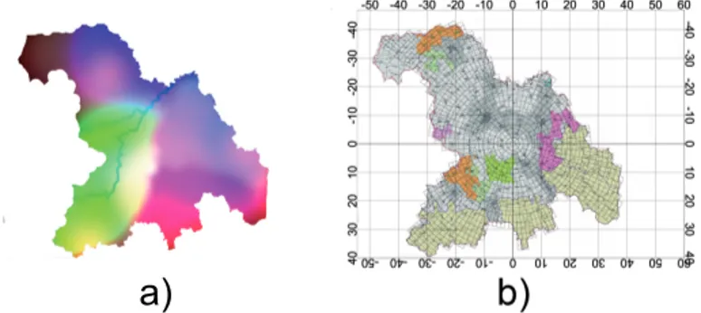
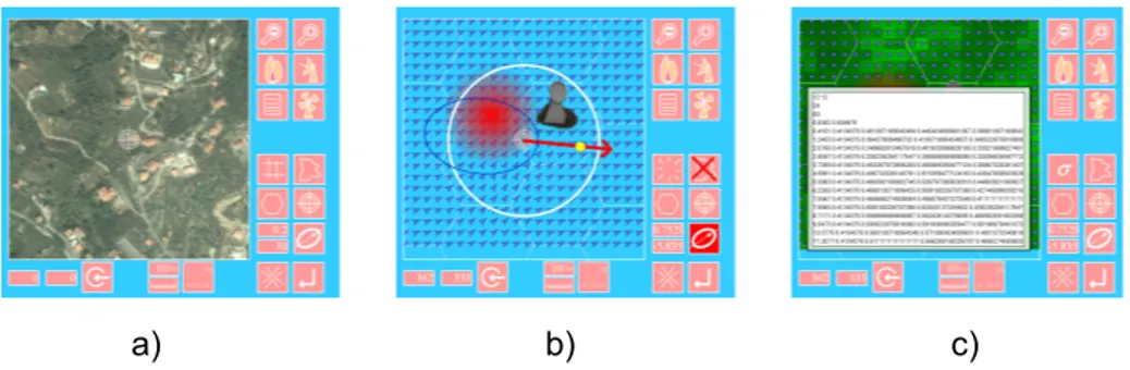
For example in [9], the propagation of a disaster such as an earthquake was studied starting from maps of the considered region such as the one presented in Figure 1. In that particular case, an application capable of performing discretiza-tion over a circular or elliptic grid was used. Figure 2 shows some screen-shots of GUI of such application. The application is capable of specifying both the center of the discretization that corresponds to the epicenter of the propagation, a semi-axis and a direction in case of elliptical propagation. The output of the tool consists in a list of cells, each characterized by its own parameters derived from the associated map.
Fig. 1. Color coded maps of the model parameters: a) the source data; b) the discretized version .
Fig. 2. The circular/elliptic discretization Tool screen-shot: a) importing the terrain data; b) defining the center and the form of the discretization; c) the tool output .
In [10], the propagation of fire over a region was considered. In that case a simple application that extracts the agent densities and the fire-extinction rate from the RGB channels of a satellite image, and that allows the user to specify the wind direction sampled by the meteorological stations was developed. Some screen-shots of the tool interface are shown in Figure 3. The tool divides the region into square cells of equal dimensions such that the burning properties and the wind direction inside each cell can be considered constant. Also in this case the tool produces a list of cells, each characterized by the property of the corresponding area under the map.
Fig. 3. Tool screen-shot: a) importing the terrain data; b) defining the wind intensity; c) exporting the output values .
Both applications are written in Adobe Flash, and join with the MASolver can be considered as a part of a tool suite developed to allow the specification and analysis of spatial dependencies in MA models.
4
The Graph-based tool
In this work a new tool for the Graph-based specification of the interconnection among agents is introduced. This tool allows the user to define visually the interaction among the objects using a graphical user interface, and it is preferable over image-based tools when the number of objects is limited and the interactions among the components can be defined manually.
The Graph-based tool uses the DrawNet[17, 18] framework as its Graphical User Interface. DrawNet is a framework supporting the design and solution of models represented in any graph-based formalism. It is based on an open archi-tecture and uses an XML-based language to create new (multi)formalisms and model-based (multi)formalisms.
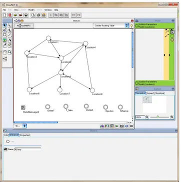
A new DrawNET formalism4called Markovian Agents Routing Graph has been implemented to define the interconnection graph of stochastic models based on multi-hop networks. The formalism allows the user to edit the following objects: i) Location Nodes, ii) the Message Service Rates and iii) a set of Parameters used to define the solution. Locations are used to define the posi-tions of the agents in the model, and message service rates are used to specify the interconnections among the agents. An example of a model-based Markovian Agents Routing Graph is shown in Fig.4.
The built model can be exported to a plain ASCII file and made available for further processing by other tools including the MASolver. The exported data includes the Topology Incident Matrix, the Message Service Rates, the so-lution Parameters and a Distance Matrix. The Topology Incident Matrix is a matrix M where, for each pair of indexes (i, j), M [i][j] is set to 1 if there is a directed arc from Locationito Locationj (0 otherwise).The Message Service
Rates and the solution Parameters are floating point numbers; finally, the Distance Matrix is a matrix D where, for each pair of indexes (i, j), D[i][j] is calculated as the geometric distance between Locationi and Locationj. Fig.5
shows an example of output file for the previous model.
5
Computing the number of hops in critical
infrastructures with MA
In this section we provide an application of the Graph-based tool join with the
MASolver to define and analyse a case study of a simplified fault detection
distributed system monitoring an electrical power grid.
In a power grid, the nodes monitor the status of the electrical lines and signal the presence of faults to the central station by sending messages each time they detect a faulty line. These messages are transferred to the central station by means of intermediate nodes according to a multi-hop routing. Moreover, each message includes the number of hops traversed in its path to the sink. In this
4
DrawNET addresses sets of graphical primitives that can be used to design a model as formalisms
Fig. 4. A Markovian Agents Routing Graph model in DrawNet
way the central station can infer the distance from its position to the detected faulty line in terms of number of hops. Each time a node receives messages with different values of number of hops, it forwards only the message carrying the minimum value incremented by one. This is done in order to signal to the central station the minimum number of hops to reach the faulty line. This scenario is illustrated in Figure 6(b): node A receives messages from both nodes B and C with a value of hops equal to one and zero respectively, and sends to the central station S a message where the number of hops is set to one.
I 0 1 2 3 m0 m1 m2 m1 m0 m1 m0 m0 m2 m3 λ µ µ µ µ
(a) Agent Node
hp:0 hp:1 hp:1 hp:0 A B C S
(b) Multi hop routing
Fig. 6. Agent Node (a), choice of the minimum between different values of hop number (b).
Node Agent Agents belonging to the node class represent the distance of a
detected or signalled fault in their state space. It is assumed that the grid is deployed to signal the presence of fault at most at M hops from the central station, in such case each node maintains information of the presence of a fault at most at M hops. The node agent is therefore characterized by M + 2 states, and its state space is defined as Sn={I, 0, 1, . . . , M}. Nodes are represented by
a single agent MAn shown in Figure 6(a) for M = 3. The meaning of the states
is the following:
I - is the idle state: the node does not detect fault and it has not received
messages signaling the presence of it;
i - are the detection states: state 0 means that the node has detected a local
fault, state i, with 0 < i≤ M, means that the node was informed by the other ones of the presence of a fault at i hops from its position.
The local transition at a rate λ from the idle state to the state 0 indicate the detection of a local fault.
The MAn can emit and receive M + 1 types of messages (m
0, m1, ..., mM)
corresponding to the number of hops. The behavior of the MAn agent at the
reception of the messages is the following:
mi - the signal message; a message mi is sent with probability 1 at the rate µ
when the MAnsojourns in state i (shown as a self-loop in Figure 6(a)); when
the MAn is in states j and a message of type m
i is perceived, it induces a
transition to state i + 1 with probability 1 only if j = I or i + 1 < j, it is ignored otherwise. In such a way a node agent a, which is informed of a faulty line at i hops from its position, transfers one hop further this information at his neighbor node b which jumps to state i + 1. Such information is ignored if node b is already informed of a closer fault.
The nodes of the grid are connected to each other by communication links along which the messages are exchanged. This results in a communication net-work with a topology that can be represented by a graph G = (V, E), where the elements in the set V are the vertices and the elements in set E are the edges of the graph. The perception function umi(v, n, i, v0, n, i0) is built to route messages of type mi along the edges of such graph. To this end, the perception
function is defined for all the node of class n and all the message of types mias:
umi(v, n, i, v0, n, j) = 1 if (v0, v)∈ E 0 otherwise (5)
Therefore, a node v perceives messages incoming from a node v0, if and only if node v0 is directly connected with v.
5.1 Performance evaluation
For each node of the network, the main measure of interest is the evolution of the mean value of the hop-number carried by the received incoming messages. This value is computed as:
φ(t, v) =
M
X
i=0
i· ρni(t, v) (6)
For a given node v of the network at time t, such index measures on average how far (in hop units) are the sources of the incoming messages received by the node.
A practical performance index is defined as the mean time needed by a mes-sage - originated at a distance equal to a number of i hops from a node v - to be received. This index is denoted as T (v, i). Another measure of interest can be derived by calculating how quickly the central station was informed of the detection of a fault in the electrical lines of the power grid and how quickly it could recover the fault. The value of T (v, i) depends on both:
– the number of hop i needed by a message originated in the faulty section of
the grid to reach the central station;
– the mean time needed to the message to perform a single hop in its path to
the central station. Due to the exponential distribution of the time needed by a transition to be performed by an MA , this value is equal to 1/α. The index can be computed as:
T (v, i) =
Z +∞ 0
(1− ρni(t, v))dt (7)
the derivation of Eq (7) can be found in [25].
5.2 Numerical results
The indices defined in Eq (6) and (7) have been computed by means of the
MASolver under different topologies of the communication network monitoring
the power grid. The first set of experiments include two simple topologies shown in Figure 7. They are called direct ring (a) and direct ring with shortcut (b). In both cases it is assumed that the fault is originated in the section of the grid monitored by node n7. In the direct ring topology such node starts to send messages to its only neighbor node n0, n0 forwards to n1 and so on, instead in the direct ring with shortcut n7 forwards its messages to both n0 and n3, then n0forwards to n1and n3forwards to n4 and so on. In all the experiments,
λ = α = 10s−1 while the initial state of n7is set to 0, i.e. this node has detected a fault. The initial state of all other nodes is set to the idle state I.
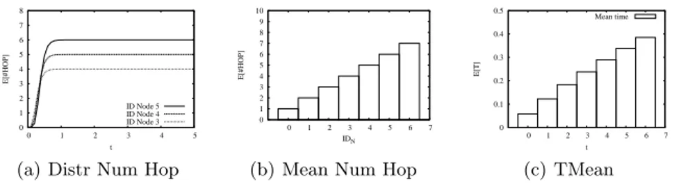
Figure 8(a) plots the evolution in time of φ(t, v), the mean value of the hop-number carried by the messages received by the nodes n3, n4 and n5. It can be observed that these values are equal to zero at t = 0 and then converge to the exact number of hops that separate them to the node n7. Set t to the time of convergence, Figure 8(b) shows the node identifier nion the x-axis and the value
of φ(t, ni) on the y-axis. For all the nodes, this value is equal to the distance
in number of hops to the node n7, which confirms that the defined behavior of the MAs allows to compute correctly in a distributed way the number of hops between node n7 and all the other nodes of the network. Finally, Figure 8(c) plots for each node of the network the value of T (ni, j) with j equal to the exact
distance in number of hops between the node itself and the node n7. This value is the time interval needed by a message originated from node n7to reach the other nodes ni. The expected trend obtained in the figure is due to the topology of
the network. This time interval is proportional to m∗ K, where m is the number of hops performed and K is a constant equal to the time needed to perform a single hop.
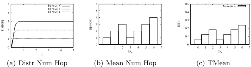
The second topology was designed to test whether the defined behavior of the MAs allows not only to compute the number of hops, but also the minimum value of them. To this end, it has been added a shortcut to the ring topology allowing the message originated from node n7to reach some nodes with less hops. Figure
9 plots for the ring with shortcut case the same set of results previously shown for the ring topology. The minimum value is computed correctly in this case as well. For example, node n3 can be reached by node n7 in two ways: along the path n7→ n0→ n1→ n2→ n3 with four hops or directly through the shortcut with one hop. As shown in Figure 9(b), the last path with the minimum number of hop was correctly chosen.
n 0 n1 n2 n 7 n3 n 6 n5 n4 (a) Ring n 0 n1 n2 n 7 n3 n 6 n5 n4 (b) Ring Short
Fig. 7. Topologies: Direct Ring (a), Direct Ring with shortcut.
0 1 2 3 4 5 6 7 8 0 1 2 3 4 5 E[#HOP] t ID Node 5 ID Node 4 ID Node 3
(a) Distr Num Hop
0 1 2 3 4 5 6 7 8 9 10 0 1 2 3 4 5 6 7 E[#HOP] IDN
(b) Mean Num Hop
0 0.1 0.2 0.3 0.4 0.5 0 1 2 3 4 5 6 7 E[T] t Mean time (c) TMean
Fig. 8. Topology: ring. Time evolution of the mean hop number to reach each node (a), mean hop number to reach each node in steady state (b), mean time T (v, i) (c).
A final case was used to test a complex topology. This included a random net-work - generated by using the functionality of the tool Pajek - and the computed value of φ(t, ni). Pajek [2] is a tool developed by the University of Ljubljana for
the generation and analysis of large networks. Given a set of parameters (e.g. number of nodes, connectivity degree distribution, ecc...) this tool is able to gen-erate automatically a random network with specific characteristics, moreover it can export the network in standard formats such as adjacency matrix, adjacency list or others. The network produced by Pajek is shown in Figure 10(a), whereas Figure 10(b) plots for each node nithe value of φ(t, ni). Also, in complex random
0 1 2 3 4 5 1 2 3 4 5 E[#HOP] t ID Node 2 ID Node 3 ID Node 4
(a) Distr Num Hop
0 1 2 3 4 5 6 1 2 3 4 5 6 7 E[#HOP] IDN
(b) Mean Num Hop
0 0.1 0.2 0.3 0.4 0.5 0 1 2 3 4 5 6 7 E[T] IDN Mean time (c) TMean
Fig. 9. Topology: ring with shortcut. Time evolution of the mean hop number to reach each node (a), mean hop number to reach each node in steady state (b), mean time
T (v, i) (c). n 1 n3 n2 n 0 n 5 n 4 n 9 n 7 n 6 n 8 (a) Random Topology
0 1 2 3 4 5 6 7 8 9 10 0 1 2 3 4 5 6 7 8 9 10 E[#HOP] IDN
(b) Mean Num Hop
Fig. 10. Random topology (a), mean hop number to reach each node in steady state (b).
6
Conclusions
In this work the problem of considering spatial aspects and performance models in MAs has been considered. A review of some of the available tools has been provided, and a new tool for the definition of graph-based interactions has been introduced. To demonstrate how the tool works, an application including a power grid critical infrastructure has been presented.
The graph-based and the image-based tools considered in this work, although intended for MAs, can be applied also to other spatial formalisms (such as CAs or SPAs). Currently, the presented tools are still in an experimental phase; future works aim at integrating them into a multi-formalism environment to allow full analysis of MA and SPA models.
Acknowledgments
This work has been partially supported by Regione Piemonte within the frame-work of the “M.A.S.P.” project POR FESR 2007/2013 -Misura I.1.3 “Poli di Innovazione - Polo Information & Communication Technology”.
References
1. N. Anastasiou, T.-C. Horng, and W. Knottenbelt. Deriving generalised stochas-tic petri net performance models from high-precision location tracking data. In
Proceedings of the ValueTools 2011, ValueTools 2011. IEEE, 2011.
2. V. Batagelj and A. Mrvar. Pajek - analysis and visualization of large networks. In
Graph Drawing Software, pages 77–103. Springer, 2003.
3. A. Bobbio, G. Bonanni, E. Ciancamerla, R. Clemente, A. Iacomini, M. Minichino, A. Scarlatti, R. Terruggia, and E. Zendri. Unavailability of critical SCADA com-munication links interconnecting a power grid and a telco network. Reliability
Engineering and System Safety, 95:1345–1357, 2010.
4. A. Bobbio, D. Cerotti, and M. Gribaudo. Presenting dynamic markovian agents with a road tunnel application. In MASCOTS09. IEEE-CS, 2009.
5. A. Bobbio, R. Terruggia, A. Boellis, E. Ciancamerla, and M. Minichino. A tool for network reliability analysis. In F. Saglietti and N. Oster, editors, Int. Conference
on Computer Safety, Reliability and Security, SAFECOMP2007, pages 417–422.
Springer Verlag - LNCS, Vol 4680, 2007.
6. G. Bonanni, E. Ciancamerla, M. Minichino, R. Clemente, A. Iacomini, A. Scar-latti, E. Zendri, and R. Terruggia. Exploiting stochastic indicators of interdepen-dent infrastructures: the service availability of interconnected networks. In Safety,
Reliability and Risk Analysis: Theory, Methods and Applications, volume 3. Taylor
and Francis, 2009.
7. Dario Bruneo, Marco Scarpa, Andrea Bobbio, Davide Cerotti, and Marco Grib-audo. Markovian agent modeling swarm intelligence algorithms in wireless sensor networks. Performance Evaluation, In Press, Corrected Proof:–, 2011.
8. Davide Cerotti. Interacting Markovian Agents. PhD thesis, Universita degli Studi di Torino, 2010.
9. Davide Cerotti, Marco Gribaudo, and Andrea Bobbio. Disaster propagation in heterogeneous media via markovian agents. In CRITIS, pages 328–335, 2008. 10. Davide Cerotti, Marco Gribaudo, Andrea Bobbio, Carlos Miguel Tavares Calafate,
and Pietro Manzoni. A markovian agent model for fire propagation in outdoor environments. In EPEW, pages 131–146, 2010.
11. C.F. Chiasserini, R. Gaeta, M. Garetto, M. Gribaudo, D. Manini, and M. Sereno. Fluid models for large-scale wireless sensor networks. Performance Evaluation, 64(7-8):715 – 736, 2007.
12. European commission: http://europa.eu/rapid/pressReleasesAction.do?reference=MEMO/06/477, 2006.
13. A. Dunn. A model of wildfire propagation using the interacting spatial automata
formalism. PhD thesis, University of Western Australia, 2007.
14. Vashti Galpin. Modelling network performance with a spatial stochastic process algebra. Advanced Information Networking and Applications, International
15. S. Di Gregorio, R. Rongo, R. Serra, W. Spataro, G. Spezzano, D. Talia, and M. Vil-lani. Parallel simulation of soil contamination by cellular automata. In Parcella, pages 295–297, 1996.
16. M. Gribaudo, D. Cerotti, and A. Bobbio. Analysis of on-off policies in sensor networks using interacting markovian agents. In PerCom, pages 300–305, 2008. 17. Marco Gribaudo, Daniele Codetta Raiteri, and Giuliana Franceschinis. Drawnet,
a customizable multi-formalism, multi-solution tool for the quantitative evaluation of systems. In QEST, pages 257–258, 2005.
18. DrawNet Project: http://www.draw net.com, 2011.
19. A. Jimnez and A. M. Posadas. A moore’s cellular automaton model to get prob-abilistic seismic hazard maps for different magnitude releases: A case study for greece. Tectonophysics, 423(1-4):35 – 42, 2006.
20. Timothy C. Matisziw and Alan T. Murray. Modeling s-t path availability to sup-port disaster vulnerability assessment of network infrastructure. Comput. Oper.
Res., 36:16–26, January 2009.
21. J. V. Neumann. Theory of Self-Reproducing Automata. University of Illinois Press, Champaign, IL, USA, 1966.
22. M. Opper and D. Saad. Advanced Mean Field Methods: Theory and Practice. MIT University Press, 2001.
23. P. Siregar, J. P. Sinteff, M. Chahine, and P. Lebeux. A cellular automata model of the heart and its coupling with a qualitative model. Comput. Biomed. Res., 29(3):222–246, 1996.
24. Nils Kalstad Svendsen and Stephen D. Wolthusen. Graph models of critical in-frastructure interdependencies. In Proceedings of the 1st international conference
on Autonomous Infrastructure, Management and Security: Inter-Domain Manage-ment, AIMS ’07, pages 208–211. Springer-Verlag, 2007.
25. Kishor S. Trivedi. Probability and statistics with reliability, queuing and computer
science applications. John Wiley and Sons Ltd., 2nd edition edition, 2002. pages