A
A
l
l
m
m
a
a
M
M
a
a
t
t
e
e
r
r
S
S
t
t
u
u
d
d
i
i
o
o
r
r
u
u
m
m
–
–
U
U
n
n
i
i
v
v
e
e
r
r
s
s
i
i
t
t
à
à
d
d
i
i
B
B
o
o
l
l
o
o
g
g
n
n
a
a
DOTTORATO DI RICERCA
Scienze Geodetiche e Topografiche
Ciclo XX
Settore scientifico disciplinare di afferenza: ICAR06
TITOLO TESI
Monitoring Ice Velocity Field in Victoria Land (Antarctica) Using
Cross-Correlation Techniques on Satellite Images
Presentata da:
Ivano Pino
Coordinatore
Dottorato Relatore
Prof.
Gabriele
Bitelli
Prof.
Gabriele
Bitelli
A
A
l
l
m
m
a
a
M
M
a
a
t
t
e
e
r
r
S
S
t
t
u
u
d
d
i
i
o
o
r
r
u
u
m
m
–
–
U
U
n
n
i
i
v
v
e
e
r
r
s
s
i
i
t
t
à
à
d
d
i
i
B
B
o
o
l
l
o
o
g
g
n
n
a
a
DOTTORATO DI RICERCA
Scienze Geodetiche e Topografiche
Ciclo XX
Settore scientifico disciplinare di afferenza: ICAR06
TITOLO TESI
Monitoring Ice Velocity Field in Victoria Land (Antarctica) Using
Cross-Correlation Techniques on Satellite Images
Presentata da:
Ivano Pino
Coordinatore
Dottorato Relatore
Prof.
Gabriele
Bitelli
Prof.
Gabriele
Bitelli
Key Words: Cross-Correlation Global Change Ice Velocity Image Enhancement Multisensor Orthorectification
Dedication
(Dedica)
_______________
To my family
(Alla mia famiglia)
Preface
The large ice sheets of Antarctica and Greenland are immensely important in the global climate system, occupying about 11% of the Earth’s land surface. In spite of its importance, the mass balance (the net volumetric gain or loss) of the Antarctic ice sheet is poorly known; it is not known exactly whether the ice sheet is growing or shrinking. Changes in the area and volume of the polar ice sheets are strictly linked to global changes and could result in sea-level variation that would severely affect the densely populated coastal regions on the Earth.
Velocity of ice-streams is a critical parameter, which, together with ice thickness, allows the determination of ice discharge rates; this information is however in large part not available, or only partially available for the last years, and can be mainly provided by using remote sensing technologies and techniques.
Antarctica is the only continent which has still to be fully explored [144]. Because of its geographical position and physical characteristics, together with the distance from sources of pollution and the almost total absence of anthropic disturbance, Antarctica provides us with a unique opportunity to obtain data for a global knowledge of the planet [144]. Antarctica is perhaps the continent in which the nations respond more freely to the need for common research programmes. A Treaty was signed in Washington on December 1st 1959 by the 12 countries participating in the International Geophysical Year (1957-1958); the Treaty covers the area south of 60°S latitude. Its objectives are simple yet unique in international relations, being:
- to demilitarize Antarctica, to establish it as a zone free of nuclear tests and the disposal of radioactive waste, and to ensure that it is used for peaceful purposes only;
- to promote international scientific cooperation in Antarctica; - to set aside disputes over territorial sovereignty.
The Antarctic Treaty remains in force indefinitely. The success of the Treaty has been the growth in membership. Forty six countries, comprising around 80% of the world’s population, have acceded to it. Consultative (voting) status is open to all countries who have demonstrated their commitment to the Antarctic by conducting significant research.
In the context of the research in Antarctica, Italian contribution is developed by the Italian National Antarctic Research Programme (Programma Nazionale di Ricerca in Antartide, PNRA), active since 1985 with an expedition every year. The research Programme includes many disciplines: Earth Sciences, Atmosphere Physics, Cosmology, Biology and Medicine, Oceanography, Environmental Sciences, Technology. During its development, the Programme increasingly addressed the study of global phenomena inside the atmosphere, the biosphere, and the geosphere. PNRA has its main base at Mario Zucchelli Station in Terra Nova Bay, lying between Cape Washington and the Drygalski Ice Tongue along the coast of Victoria Land. Logistic and research facilities allow there the execution of activities in the main research fields and in the framework of major international projects. Other important research activities are carried out at the Concordia Station, recently completed in collaboration with France, built 3233 m above sea level at a location called Dome C on the Antarctic Plateau; Concordia Station is located 1200 kilometres inland from Mario Zucchelli Station. This site was chosen by the European Project for Ice Coring in Antarctica
2007-2008 has been appointed as the International Polar Year. Since the first International Polar Year in 1882-83 there have been a number of major international science initiatives in Polar Regions and all have had a major influence in providing a better understanding of global processes in these areas. These initiatives have involved an intense period of interdisciplinary research, collecting a broad range of measurements that provide a snapshot in time of the state of the polar regions. As mentioned, a fundamental moment was the International Geophysical Year 1957-58, involving 80000 scientists from 67 countries: it produced new explorations and discoveries in many fields of research and changed in a fundamental manner how science was conducted in the polar regions. Fifty years on, technological developments such as growing availability of earth observation satellites, autonomous vehicles and molecular biology techniques offer enormous opportunities for a further step in our understanding of polar systems.
The International Polar Year (IPY) 2007-2008, actually running from March 2007 to March 2009, is then an international programme of coordinated, interdisciplinary scientific research and observations in the Earth's polar regions with the aim to:
- explore new scientific frontiers;
- deepen our understanding of polar processes and their global linkages;
- increase our ability to detect changes, to attract and develop the next generation of polar scientists, engineers and logistics experts;
- capture the interest of schoolchildren, the public and decision-makers.
Focus areas of IPY campaigns are Atmosphere, Ice, Land, Oceans, People, Space.
One might ask what are or what will be the advantages of the research activities performed in Antarctica, considering the financial effort they require. The answer is essentially "knowledge". Research activity does not necessarily engender immediate tangible results. The product is the outcome of slow maturation and derives from the combination of results obtained by the various countries in the various sectors of research.
The introduction of the Thesis focus on the Global Change problem and the linkage with ice flows behaviour in polar regions. Chapter 2 describes remote sensing observation of ice sheets and glaciers and their characterization. Third chapter describes the most utilized approaches to the determination of ice motion. Chapter 4 and 5 are related to the study of an ice flow (David glacier) carried out by a multitemporal analysis developed using imagery coming from different sensors (MSS, TM, ETM+, ASTER, HRVIR) on board of different satellites (Landsat, Terra and Spot). The images were acquired from 1973 to 2006 and the scenes cover about 200 km of the coastal zone in Victoria Land (Terra Nova Bay); the major glaciers of Victoria Land flow into this bay. Mario Zucchelli Station, formerly known as Terra Nova Bay Station, is located along the coast of the northern foothills between the Campbell and Drygalski glacier tongues.
The study, mainly concentrated on the monitoring of David glacier, seeks to develop a methodology aiming to reach the following objectives:
- multisensor satellite data integration using image cross-correlation techniques, in order to measure ice displacements;
- enhancement of measurement precision by image processing techniques and filtering methodologies, also applying GIS techniques;
- accuracy assessment and comparison with the results obtained using different methods and surveying techniques.
Acknowledgements
SPOT images are provided thought OASIS (Optimizing Access to SPOT Infrastructure for Science), European project coordinated by CNES and financed by the European Commission. ASTER images are provided through a grant with NASA (National Aeronautics and Space Administration, USA).
ENEA (Ente per le Nuove tecnologie, l’Energia e l’Ambiente) “Casaccia” Research Centre, Roma, provided MSS, TM and some ETM+ Landsat images through a research collaboration with Dr. Massimo Frezzotti.
Table of Contents
Chapter 1 Introduction
1
Chapter 2 Remote Sensing of Glaciers and Ice Sheets
11
2.1 Introduction 11
2.2 Remote Sensing Techniques 11
2.3 Ice Sheet and Glaciers 14
2.4 Physical Characterization 15
2.5 Electromagnetic Properties in the Optical and Near Infrared Regions 18 2.6 Mass Balance 18
Chapter 3 Ice
Velocity
Measurement
by
Satellite
21
3.1 Introduction 21
3.2 Remote Sensing Techniques 22
3.2.1 Visual-based Photogrammetric method 22
3.2.2 Image Cross-Correlation 22 3.2.3 SAR Interferometry 24
3.3 Global Positioning System 27
Chapter 4 Determination of Ice Velocity Field: Instruments
29
4.1 Introduction 294.2 Physical Basis of Remote Sensing 29
4.3 Resolution and Sampling in Remotely Sensed Data 31
4.4 Electro-Optical System in the Visible and Near-Infrared Region 32 4.5 Satellite-borne multispectral system 34
4.5.1 Landsat 1 - Mulltispctral Scanner System (MSS) 34
4.5.2 Landsat 4 - Thematic Mapper (TM) 35
4.5.3 Landsat 7 - Enhanced Thematic Mapper Plus (ETM+) 36 4.5.4 SPOT 4 - High Resolution Visible Infra Red (HRVIR) 38 4.5.5 Terra-ASTER VNIR Sub-System 39
Chapter 5 Monitoring of David Glacier in Victoria Land: Method and
Application
43
5.1 Introduction 43 5.2 Image Preprocessing 45 5.2.1 Band Transformation 47 5.2.2 Radiometric Correction 47 5.2.3 Geometric Correction 48 5.2.4 Radiometric Enhancement 55 5.3 Cross-Correlation Processing 57 5.4 Post-Processing 60 5.4.1 Fine Coregistration 60 5.4.2 Output Filtering 60 5.4.3 Assessment Accuracy 63 5.5 Method Validation 655.6 David Glacier Monitoring 68
Chapter 6 Conclusions
72
Appendix
1:
Principal
Component
Analysis
74
Appendix
2:
Direct
Orthorectification
Model
75
Appendix 3: Root Mean Square Deviation (or Error)
80
Appendix
4:
Spatial
Filtering
81
Appendix
5:
Histogram
Equalization
83
Appendix 6: Automatic Displacement Filtering (MATLAB)
85
Appendix
7:
Propagation
of
Uncertainty
89
Chapter 1
Introduction
Although the Earth system is constantly changing, ozone depletion, increases in atmospheric greenhouse gases, large-scale pollution and changing patterns of natural resource use demonstrate that human activities are altering the Earth system at an accelerated pace. Awareness of this has led to an evolving international consensus on the importance of both increasing our scientific understanding of global change and linking scientific findings to policy decisions [139].
Climate change is one of the most critical global challenges of our time. Recent events have emphatically demonstrated our growing vulnerability to climate change. Climate change impacts will range from affecting agriculture, further endangering food security, sea-level rise and the accelerated erosion of coastal zones, increasing intensity of natural disasters, species extinction and the spread of vector-borne diseases [145]. In recent usage, especially in the context of environmental policy, the term "climate change" often refers to changes in modern climate, consequences of global warming phenomenon, that represents the increase in the average temperature of the Earth's near-surface air and oceans in recent decades (Figure 1.1) and its projected continuation (Figure 1.5) [129]. In common usage, the term refers to recent warming and implies a human influence [50]. The United Nations Framework Convention on Climate Change (UNFCCC) uses the term "climate change" for human-caused change, and "climate variability" for other changes [111]. The term "anthropogenic global warming" is sometimes used when focusing on human-induced changes.
The Intergovernmental Panel on Climate Change (IPCC) is a scientific body tasked to evaluate the risk of climate change caused by human activity [129]. The panel was established in 1988 by the World Meteorological Organization (WMO) and the United Nations Environment Programme (UNEP), two organizations of the United Nations. IPCC concludes "most of the observed increase in globally averaged temperatures since the mid-20th century is very likely due to the observed increase in anthropogenic greenhouse gas concentrations"[47] via the greenhouse effect (Figure
1.2). The greenhouse effect is the process in which the emission of infrared radiation by the
atmosphere warms a planet's surface. The name comes from an incorrect analogy with the warming of air inside a greenhouse compared to the air outside the greenhouse [129]. The Earth's average surface temperature of 15 °C is about 33 °C warmer than it would be without the greenhouse effect [48]. Understanding global warming requires understanding the changes in climate forcings that have occurred since the industrial revolution. These include positive forcing from increased greenhouse gases, negative forcing from increased sulphate aerosols and poorly constrained forcings from indirect aerosol feedbacks as well as minor contributions from solar variability and other factors. The poorly constrained aerosol effects results from both limited physical understanding of how aerosols interact with the atmosphere and limited knowledge of aerosol concentrations during the pre-industrial period. Contrary to the impression given by Figure 1.3, it is not possible to simply sum the radiative forcing contributions from all sources and obtain a total forcing. This is because different forcing terms can interact to either amplify or interfere with each other. For example, in the case of greenhouse gases, two different gases may share the same absorption bands thus partially limiting their effectiveness when taken in combination. This is a
significant source of uncertainty in comparing modern climate forcings to past states [129].
FIGURE_1. 1: Global mean surface temperature anomaly 1850 to 2007 relative to 1961-1990 (instrumental record of global average temperatures as compiled by the Climatic Research Unit of the University of East Anglia and the Hadley Centre of the UK Meteorological Off
FIGURE_1.2: Climate change attribution. This figure, based on Meehl et al. 2004 [84 ], shows the ability of a global climate model (the DOE PCM [57][58]) to reconstruct the historical temperature record and
FIGURE_1. 3: Components of the current radiative forcing as estimated by the IPCC Fourth Assessment Report (1750-2005).
Figure 1.4 shows the variations in concentration of carbon dioxide (CO2) in the atmosphere during
the last 400 thousand years. Throughout most of the record, the largest changes can be related to glacial/interglacial cycles within the current ice age. Although the glacial cycles are most directly caused by changes in the Earth's orbit (i.e. Milankovitch cycles), these changes also influence the carbon cycle, which in turn feeds back into the glacial system. Since the Industrial Revolution, circa 1800, the burning of fossil fuels has caused a dramatic increase of CO2 in the atmosphere, reaching levels unprecedented in the last 400 thousand years. This increase has been implicated as a primary cause of global warming.
Natural phenomena such as solar variation combined with volcanoes probably had a small warming effect from pre-industrial times to 1950 and a small cooling effect from 1950 onward [44][1]. These basic conclusions have been endorsed by at least 30 scientific societies and academies of science [106], including all of the national academies of science of the major industrialized countries [99][97][89]. While individual scientists have voiced disagreement with some findings of the IPCC [81], the overwhelming majority of scientists working on climate change agree with the IPCC's main conclusions [98][107].
The global average air temperature near the Earth's surface rose 0.74 ± 0.18°C (1.33 ± 0.32°F) during the 100 years ending in 2005 [47]. Climate model projections summarized by the IPCC indicate that average global surface temperature will likely rise a further 1.1 to 6.4°C (2.0 to 11.5°F) during the 21st century [47]. The range of values results from the use of differing scenarios of future greenhouse gas emissions as well as models with differing climate sensitivity.
Although most studies focus on the period up to 2100, warming and sea level rise are expected to continue for more than a thousand years even if greenhouse gas levels are stabilized. The delay in reaching equilibrium is a result of the large heat capacity of the oceans [85]. Figure 1.5 shows a projection of the geographic distribution of surface warming during the 21st century from Hadley Centre HadCM3 climate model [143]. As can be expected from their lower specific heat, continents warm more rapidly than the oceans in the model with an average of 4.2°C to 2.5°C respectively. The lowest predicted warming is 0.55°C south of South America, and the highest is 9.2°C in the Arctic Ocean (points exceeding 8°C are plotted as black). This model is fairly homogeneous except for strong warming around the Arctic Ocean related to melting sea ice and strong warming in South America related predicted changes in the El Niño cycle, that is part of a interannual cycle called ENSO (El Nino, Southern Oscillation) which occurs in the tropical waters of the Pacific Ocean (El Nino is the warm part of this cycle. It occurs once every 3 to 7 years).
Increasing temperatures tend to increase evaporation, which leads to more precipitation [47]. As average global temperatures have risen, average global precipitation has also increased. According to the IPCC, the following precipitation trends have been observed:
• Precipitation has generally increased over land north of 30°N from 1900-2005, but has mostly declined over the tropics since the 1970s. Globally there has been no statistically significant overall trend in precipitation over the past century, although trends have widely by region and over time.
• It has become significantly wetter in eastern parts of North and South America, northern Europe, and northern and central Asia, but drier in the Sahel, the Mediterranean, southern Africa and parts of southern Asia.
• Changes in precipitation and evaporation over the oceans are suggested by freshening of mid- and high-latitude waters (implying more precipitation), along with increased salinity in low-latitude waters (implying less precipitation and/or more evaporation).
• There has been an increase in the number of heavy precipitation events over many areas during the past century, as well as an increase since the 1970s in the prevalence of droughts especially in the tropics and subtropics.
FIGURE_1. 2: Carbon dioxide variation during the last 400 thousand years
FIGURE_1. 3: Predicted surface temperature changes expressed as the average prediction for 2070-2100 relative to the model's baseline temperatures in 1960-1990, calculated by the HadCM3 climate
In the Northern Hemisphere's mid- and high latitudes, the precipitation trends are consistent with climate model simulations that predict an increase in precipitation due to human-induced warming [141]. By contrast, the degree to which human influences have been responsible for any variations in tropical precipitation patterns is not well understood or agreed upon, as climate models often differ in their regional projections [47].
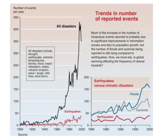
Increasing dramatic weather catastrophes are due to an increase in the number of severe events (Figure 1.6) and an increase in population densities, which increase the number of people affected and damage caused by an event of given severity. The World Meteorological Organization [16] and the U.S. Environmental Protection.
Agency [110] have linked increasing extreme weather events to global warming, as have Hoyos et
al. (2006), writing that the increasing number of category 4 and 5 hurricanes is directly linked to
increasing temperatures [45]. Similarly, Kerry Emmanuel in Nature writes that hurricane power dissipation is highly correlated with temperature, reflecting global warming. Hurricane modeling has produced similar results, finding that hurricanes, simulated under warmer, high CO2 conditions, are more intense than under present-day conditions.
Thomas Knutson and Robert E.Tuleya of the NOAA stated in 2004 that warming induced by greenhouse gas may lead to increasing occurrence of highly destructive category-5 storms [108]. Vecchi and Soden find that wind shear, the increase of which acts to inhibit tropical cyclones, also changes in model-projections of global warming. There are projected increases of wind shear in the tropical Atlantic and East Pacific associated with the deceleration of the Walker circulation, as well as decreases of wind shear in the western and central Pacific[114]. The study does not make claims about the net effect on Atlantic and East Pacific hurricanes of the warming and moistening atmospheres, and the model-projected increases in Atlantic wind shear [114].
Increasing global temperature will cause sea level to rise. Sea-level has risen about 130 metres (400 ft) since the peak of the last ice age about 18,000 years ago. Most of the rise occurred before 6,000 years ago. From 3,000 years ago to the start of the 19th century sea level was almost constant, rising at 0.1 to 0.2 mm/yr.[50] Since 1900 the level has risen at 1 to 2 mm/yr; since 1993 satellite altimetry from TOPEX/Poseidon indicates a rate of rise of 3.1 ± 0.7 mm yr–1 [15]. Church and White (2006) found a sea-level rise from January 1870 to December 2004 of 195 mm, a 20th century rate of sea-level rise of 1.7 ±0.3 mm per yr and a significant acceleration of sea-level rise of 0.013 ± 0.006 mm per year per yr. If this acceleration remains constant, then the 1990 to 2100 rise would range from 280 to 340 mm,[15].
Figure 1.7 shows the change in annually averaged sea level at 23 geologically stable tide gauge
sites with long-term records as selected by Douglas (1997) [19]. The thick dark line is a three-year moving average of the instrumental records. This data indicates a sea level rise of ~18.5 cm from 1900-2000. Because of the limited geographic coverage of these records, it is not obvious whether the apparent decadal fluctuations represent true variations in global sea level or merely variations across regions that are not resolved. For comparison, the recent annually averaged satellite altimetry data [19] from TOPEX/Poseidon are shown in red.
These data indicate a somewhat higher rate of increase than tide gauge data, however the source of this discrepancy is not obvious.
Changes in global climate and sea level are intricately linked to changes in the area and volume of polar ice sheets [72].
During the most recent glacial maximum, about 18,000 years ago, the total volume of ice was about 2.5 times, and the total area about three times, their present values [28] with the consequence that sea level was about 125m below its present level [23]. During the last glacial minimum, about
FIGURE_1. 4: Trends in natural disasters.
120,000 years ago, sea level was about 6m higher than today, and it is possible that the Greenland ice sheet largely disappeared [63]. The Little Ice Age was a period from about 1550 to 1850 when the world experienced relatively cooler temperatures compared to the present. Until about 1940, glaciers around the world retreated as the climate warmed. Glacial retreat slowed and even reversed, in many cases, between 1950 and 1980 as a slight global cooling occurred. However, since 1980 a significant global warming has led to glacier retreat becoming increasingly rapid and ubiquitous, so much so that some glaciers have disappeared altogether, and the existence of a great number of the remaining glaciers of the world is threatened. In locations such as the Andes of South America and Himalayas in Asia, the demise of glaciers in these regions will have potential impact on water supplies. The retreat of mountain glaciers, notably in western North America, Asia, the Alps, Indonesia and Africa, and tropical and subtropical regions of South America, has been used to provide qualitative evidence for the rise in global temperatures since the late 19th century [51][82]. The recent substantial retreat and an acceleration of the rate of retreat since 1995 of a number of key outlet glaciers of the Greenland and West Antarctic ice sheets, may foreshadow a rise in sea level, having a potentially dramatic effect on coastal regions worldwide [129]. Other large-scale phenomena that may be associated with global climate change include the possible destabilization and disintegration of the Antarctic ice shelves unstable [86]. Dramatic calving events (breaking away of ice) have been monitored [91]. In particular, it has been suggested that the West Antarctic ice sheet may be using satellite data. The Larsen ice shelf has been retreating since the 1940s, increasingly rapidly since about 1975 (Figure 1.8). Major calvings have occurred since 1986 [96], associated with acceleration of the glaciers that formerly fed the ice shelf, and the retreat is probably now irreversible [18] [102].
The respective communities have begun to communicate, linking their datasets to provide an important basis to assess ongoing climate and glacier change, and to develop realistic scenarios for future conditions and challenges in glacierised mountain regions [104]. Fluctuations of glaciers and ice caps have been systematically observed and measured for more than a century in various parts of the world [38]. They are considered to be highly reliable indications of worldwide warming trends [49]. Mountain glaciers and ice caps are, therefore, key variables to monitor for early detection strategies of global climate-related observations [104].
Since the beginning of the internationally-coordinated collection of information on glacier changes was initiated in 1894 [33], various aspects have evolved in striking ways [104]:
• Accelerating glacier shrinkage at the century time scale is now clearly non-cyclic, therefore there is little question that the originally envisaged “variations périodiques des glaciers” does not apply to ongoing developments [104];
• As a consequence of the growing influence of human impact on the climate system (enhanced greenhouse effect), dramatic scenarios of projected changes including complete deglaciation of entire mountain ranges must be taken into consideration [39]; [84]; [123]; • Such future scenarios may be beyond the range of historical/Holocene variability and most
likely introduce dramatic consequences (i.e., extent and rate of glacier melt and disequilibrium of glacier/ climate relationships) [104].
• The comparison of modern glacier retreat with the Holocene glacier variations provides important background information for our understanding of natural trends of, and human impacts on, climate change [104].
• A broad portion of the global community today recognizes glacier changes as a key indication of regional and global climate, and environment change [104];
• Observational strategies established by expert groups within international monitoring programmes build on advances in understanding processes and now include extreme perspectives [104];
• These strategies make use of the rapid development of new technologies and relate them to traditional approaches in order to apply integrated, multilevel concepts (in situ measurements to remote sensing, local-process oriented to regional and global coverage), within which individual observational
• components (length, area, volume/ mass change) fit together enabling a more holistic view of the cryosphere [10].
The link between historical and past glacier variations and climate can be made through numerical models. Such models can provide deeper insights concerning past climate and glacier dynamics [40][83][67] and several studies have made use of modelling approaches to derive information related to climate change over different timescales from glacier variations [124][104][62].
As well as their role as indicators of climate they can represent hazards through a variety of mechanisms [118] including advance, retreat and surges, release of ice-dammed lakes, iceberg discharge, and rapid disintegration [91].
There is thus a need to measure and monitor a range of properties of ice sheets and glaciers, including the ice volume and extent, distribution of surface features related to the temperature and wind regime [14][32], dynamics, and mass balance. As with snow cover, measurement of the surface albedo is also important, since it gives the possibility of modelling the energy balance of a glacier. Space-born techniques offer major advantages over in situ measurements in all of these cases [91]. Satellite remote sensing has revolutionized ice sheet research [9]. A variety of instruments sensitive to different parts of the electromagnetic spectrum take what the human eye detects as a flat, white desert and provide data sets rich in scientific information [9].
Remote sensing of terrestrial ice masses (glaciers, ice caps, and ice sheets) is generally a well-developed field. Remotely sensed data are regularly used to compile inventories and surveys of glaciers in Europe and the United States. Since 1999, the international GLIMS_ (Global Land Ice Measurements from Space) project has been carrying out routine monitoring of glaciers worldwide, using data from the ASTER and ETM+ sensors [60].
Melting of the ice sheets may severely impact the densely populated coastal regions on Earth [72]. Melting of the West Antarctic ice sheet alone could raise sea level by approximately 5 m [72]. In spite of their importance, the current mass balances (the net gains or losses) of the Antarctic ice sheets are not known. Because of difficult logistic problems in Antarctica, field research has focused on only a few major ice streams and outlet glaciers [72]. Yet, to understand the ice sheet dynamics fully, we must carefully document all of the coastal changes associated with advance and retreat of ice shelves, outlet glaciers, and ice streams [72]. A critical parameter of ice sheets is their velocity field, which, together with ice thickness, allows the determination of discharge rates [72]. Remote sensing, using moderate- to high- resolution satellite images, permits glacier movement to be measured on sequential images covering the same area; the velocities can be measured quickly and relatively inexpensively by tracking crevasses or other patterns that move with the ice [72]. Especially important are velocities where the ice crosses the glaciers grounding lines (locations along the coast where the ice is no longer ground supported and begins to float) [72].
Remote sensing has served as an efficient method of gathering data about glaciers since its emergence. The recent advent ofGeographic Information Systems (GIS) and Global Positioning
identifiable from aerial photographs and satellite imagery includespatial extent, transient snowline, equilibrium line elevation,accumulation and ablation zones, and differentiation of ice/snow.Digital image processing (e.g., image enhancement, spectral rationing and automatic classification) improves the ease andaccuracy of mapping these parameters. The traditional visiblelight/infrared remote sensing of two-dimensional glacier distribution has been extended to three-dimensional volume estimation anddynamic monitoring using radar imagery and GPS. Longitudinalvariations in glacial extent have been detected from multi-temporal images in GIS. However, the detected variations have neitherbeen explored nor modelled from environmental and topographicvariables. GPS has been utilized independent of remote sensingand GIS to determine glacier ice velocity and to obtain informationabout glacier surfaces. Therefore, the potential afforded bythe integration of non-conventional remote sensing (e.g., SARinterferometry) with GIS and GPS still remains to be realized in glaciology. The emergence of new satellite images will make remote sensing of glaciology more predictive, more global andtowards longer terms.
Figura 1.5: Larsen B Ice Shelf collapsing in Antarctica. Source: Moderate Resolution Imagin Spectroradiometer (MODIS), NASA Terra satellite, National Snow and Ice data Canter, University of Colorado [136]
Chapter 2
Remote Sensing of Ice Sheets and Glaciers
2.1
INTRODUCTION
The properties of a terrestrial ice mass that can be measured using remote sensing methods include its spatial extent, surface topography, bottom topography, total volume (which can be deduced from the surface and bottom topographies), surface flow field, accumulation and ablation rates (and hence mass balance), surface zonation, albedo, and changes in these quantities over time [91]. As well as its importance in indicating the total amount of ice, surface topography provides important clues about the internal structure and can reveal flow features and grounding lines [65]. The sensitivity of glaciers to climate, discussed in chapter 1, has meant that a major focus of research has been the assessment of mass balance. Various approaches have been adopted, including direct measurement, indirect approaches, for example based on estimating the altitude of the equilibrium line, and modeling. Modeling based on energy balance calculations requires accurate measurements of the surface albedo [112].
Visible–near-infrared (VIR) and synthetic aperture radar (SAR) imagery both play major roles in the remote sensing of terrestrial ice masses. Other remote sensing techniques are also important in studies of ice sheet and glaciers. Radio echo-sounding and closely related methods such as ground-penetrating radar can reveal depth and internal structure, and SAR interferometry reveals surface topography and velocity. Recently, laser profiling has demonstrated the ability to study topography in great detail, fine enough to resolve subtle surface features [91].
Remote sensing of terrestrial ice masses (glaciers, ice caps, and ice sheets) is generally a well-developed field. Remotely sensed data are regularly used to compile inventories and surveys of glaciers in Europe and the United States. The highest information density and most complete historical record for mountain glaciers are in the European mountain ranges, especially the Alps [59]. The situation in South America is much less complete [116]. The entire coastal zone of Antarctica from the 1970s onward is being mapped ([26]; [117]. Since 1999, the international GLIMS-(Global Land Ice Measurements from Space) project has been carrying out routine monitoring of glaciers worldwide, using data from the ASTER and ETM+ sensors [60].
2.2
REMOTE SENSING TECHNIQUES
In general terms, remote sensing can be interpreted as the gathering of information about an object without physical contact. In the more useful but more restricted sense in which the term is normally employed, it refers to airborne or spaceborne observations using electromagnetic radiation. This radiation is either naturally occurring, in which case the system is said to employ passive remote
sensing, or is generated by the remote sensing instrument itself (active remote sensing) [91].
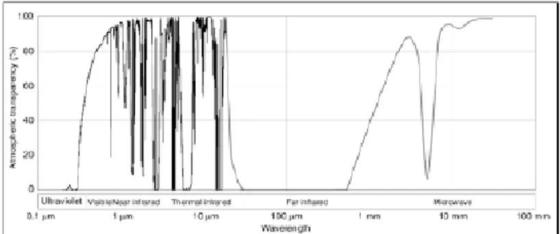
Naturally occurring radiation includes reflected solar radiation, which is largely confined to the visible and near-infrared parts of the electromagnetic spectrum (wavelengths between roughly 0.35 and 2.5 μm) and thermally emitted radiation. The range of wavelengths generated by a thermally emitting body depends on the temperature. The dominant wavelength is approximately A/T, where T is the absolute temperature of the body and A is a constant with a value of about 0.003 Km, so for a body at a temperature of 273K (0°C) the dominant wavelength is around 11 μm. The distribution of energy over wavelengths falls very sharply for shorter wavelengths, but at longer wavelengths the decrease is much more gradual. For this reason, thermally emitted radiation can be detected both in the thermal infrared part of the electromagnetic spectrum (wavelengths typically 8 to 14 μm) and also in the microwave region (wavelengths typically 1cm to 1m). The wavelength region between 14 μm and 1cm is largely blocked by the atmosphere. Figure 2.1 summarizes the useful regions of the electromagnetic spectrum for remote sensing and the transparency of the atmosphere [91]. Passive remote sensing systems that detect reflected solar radiation are designed to measure the radiance, i.e., the amount of radiation reaching the sensor in a particular waveband. If the amount of radiation that is incident on the Earth’s surface is known, the reflectance of the surface can be calculated (this requires that the effects of the atmosphere should be corrected). This can be said to be the primary variable that is measured by such systems [91].
profilers, while radio-frequency radiation is used by radar altimeters, impulse radar, and similar systems [91]. The second type of active system is, similarly to the passive reflective systems, primarily designed to measure the surface reflectance. However, instead of relying on incident solar radiation, the instrument illuminates the Earth’s surface and analyzes the signal returned to it [91]. This gives the possibility of much greater flexibility in the characteristics of the radiation its direction, wavelength, polarization, and time-structure (for example, it can be pulsed) can all be controlled [91]. Systems that employ this approach can generally be classed as imaging radars, since they operate in the microwave part of the electromagnetic spectrum. The primary variable measured in this case is the backscattering coefficient, a unitless quantity related to the concept of reflectance and usually specified in decibels (dB) rather than as a simple ratio or percentage. Its dependence on the imaging geometry is often important [91].
FIGURE 2. 1: Typical atmospheric transparency and principal regions of the electromagnetic spectrum. These regions can be further subdivided. The visible band is conventionally divided into the spectral colours from violet to red, while the microwave region is often is often designed by names of radar bands.
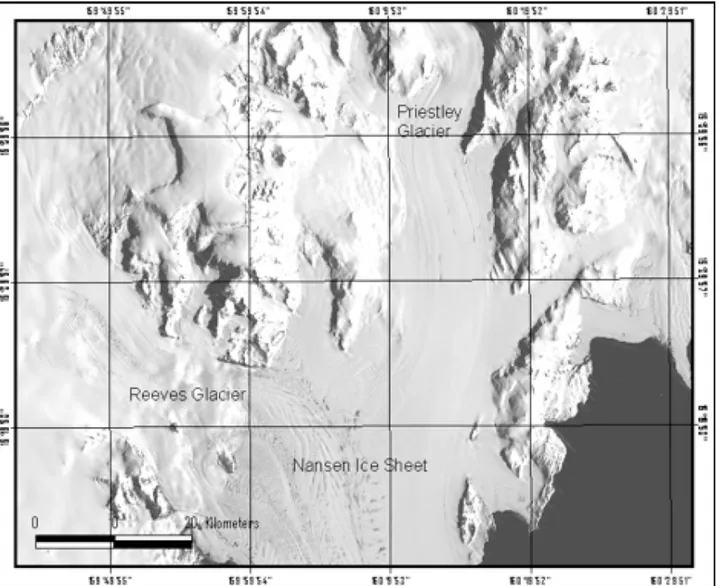
FIGURE_2. 2: Ortho image map of Terra Nova Bay (Landsat TM orthorectified image, 14 January 1992). Reeves Glacier and Priestley Glacier flow together into Nansen Ice Sheet.
2.3
ICE SHEET AND GLACIERS
Permanent snow cover eventually forms a glacier, defined as an accumulation of ice and snow that moves under its own weight. A glacier is defined as an accumulation of ice and snow that moves under its own weight [91]. Glaciers occur in a huge range of sizes, with a ratio of approximately 10 between the areas of the largest and the smallest [91]. The smallest glaciers are of the order of 10 ha (105 m2) in area, while the largest ice masses on Earth are the ice sheets of Antarctica and Greenland, representing between them about 99% of the mass and 97%of the area of land ice. Table 2.1 summarizes the global distribution of land ice [91]. The total of 3.30x10¹⁶m3 represents about 77% of the Earth’s fresh water, the remaining 23% being groundwater (22%) and lakes, rivers, snow, soil moisture, and water vapour (1%) [109]. The total discharge rate from the Earth’s land ice has been estimated as 3 1012 m3 per year [64] giving a mean residence time (the time for which a molecule of water remains as part of the glacier) of the order of 104 years [41]. This figure can be contrasted with the residence times of weeks or months for temporary and seasonal snow cover. The goal of subsequent analysis of the remotely sensed data is to interpret the value of this reflectance and its spatial and temporal variations. In the case of remote sensing systems that detect thermal radiation, the sensor again measures the radiance reaching the instrument in a particular waveband. This radiance is normally expressed as a brightness temperature, which is the temperature of a perfect emitter (a so-called black body) that would produce the same amount of radiation [91]. The primary variable to be determined is the brightness temperature of the radiation leaving the Earth’s surface (again, the effects of the atmosphere must be taken into account to relate the brightness temperature measured at the sensor to the brightness temperature leaving the surface) [91]. The brightness temperature is related to the physical temperature of the surface and its emissivity, a unitless quantity that defines the ratio of the actual radiance to the radiance that would be emitted by a black body at the same temperature [91]. It follows that the emissivity must therefore take a value between zero and unity, and that it is unity for a black body [91]. Clearly, if the emissivity of a material is known and its brightness temperature can be measured, its actual physical temperature can be calculated. Active remote sensing systems can be divided into two main types. Firstly, there are ranging instruments, whose primary purpose is to measure the distance from the sensor to the Earth’s surface by measuring the time for short pulses of radiation to travel down to the surface and back again [91]. From this information, the Earth’s surface topography can be investigated. The radiation is visible light or (more usually) near-infrared in the case of laser As indicated by Table 2.1, the two ice sheets are enormously thick — on average over 1km, and reaching a maximum thickness of 4500 m in the case of Antarctica, about 3000min Greenland. In fact, the Antarctic ice sheet is really two ice sheets, the East Antarctic and West Antarctic ice sheets, separated by the Transantarctic Mountains. The East Antarctic ice sheet is larger, thicker, and older than the West Antarctic ice sheet; the former is almost entirely above sea level, while the latter is almost entirely below it. Like all glaciers, ice sheets flow in response to gravitational forces. Faster moving regions of ice are called ice streams, essentially rivers of ice flowing across the slower-moving ice sheet. Ice also flows from the ice sheets in the form of outlet glaciers (Figure 2.1). When these reach the coast the ice continues to flow over the sea, forming an ice shelf that is anchored to the coast, as displayed in Figure 2.2, where Reeves and Priestley Glaciers flow together and form the Nansen Ice Sheet (the name given by first explorer, although it is really an ice shelf). Ice shelves are primarily an Antarctic phenomenon. Virtually all of the land area of Antarctica is covered by the ice sheet, while only about 80% of the area of Greenland is ice-covered. About 50% of the Antarctic coastline has ice shelves attached to it, the largest being the Ross ice shelf, between 200 and 1000m thick and roughly the area of France. About 11% of the area and 2.5% of the
the process is out of equilibrium in a number of cases, with ice shelves undergoing large-scale collapse [91].
Somewhat smaller than the ice sheets are the ice caps (Formally, an ice cap is up to 500,000 km2 (5 1011 m2) in area. Beyond this size it would be classed as an ice sheet), dome-shaped glaciers covering high-latitude islands or highland areas, and typically a few thousand square kilometers in extent (Figure 2.3). The major ice caps occur on Iceland, in the Canadian Archipelago, Svalbard, and the islands of the Russian Arctic. The remaining classes of glacier are the valley glaciers, which form in mountain valleys, and piedmont glaciers which form when the ice from a glacier spreads out over flatter ground (Figures 2.4). Glaciers occur on all continents except Australia. The principal glaciated areas are Alaska, Iceland, Svalbard, Norway, the Russian Arctic islands, the Alps, southern Andes, Karakoram, and Himalaya mountains [105]. Of the Earth’s glaciated area, excluding the Antarctic and Greenland ice sheets, only a few percent occurs in the southern hemisphere, predominantly in Chile [95].
2.4
PHYSICAL CHARACTERIZATION
Remote sensing, as we have already discussed and in the terms in which we have defined it, involves making inferences about the nature of the Earth’s surface from the characteristics of the electromagnetic radiation received at the sensor. This process of inference requires that we should establish the relationship between the characteristics of the radiation and the relevant physical properties of the material [91].
A glacier is a large (usually larger than 10 hectares) mass of ice having its origin on land, and normally displaying some movement. It is usually in a state of approximate dynamic equilibrium, with a net input of material in its upper accumulation area and a net loss of material in its lower ablation area. These two areas are separated by the equilibrium line. Figure 2.5 illustrates schematically the relationship between these areas and the flow of ice within the glacier. The input to a glacier is in the form of snowfall, and the output is principally in the form of melt-water and, in the case of a glacier whose lower terminus is in water, icebergs that calve off and float away. The snow is transformed to ice through a number of mechanisms [91].
The surface of a glacier can be divided into a number of zones or facies, an idea developed by Benson (1961, [4]) and Muller (1962, [79]). These are illustrated in Figure 2.6, which is adapted from [88], as is the following description. Uppermost is the dry-snow zone in which no melting takes place. This zone is only found inland in Greenland and over most of the Antarctic ice sheet, and on the highest mountain glaciers, where the annual average temperature is lower than some threshold value that was originally proposed as -25°C [4] but is now believed to be around -11°C (Peel 1992). Next is the percolation zone, in which some surface melting occurs during the summer. The meltwater percolates downward and refreezes to form inclusions of ice in the form of layers, lenses, and pipes. The dry-snow and percolation zones are separated by the dry-snow line. Below the percolation zone, and separated from it by the wet-snow line, is the wet-snow zone in which all the current year’s snowfall melts. Below this, and separated from it by the snow line (sometimes called the firn line) is the superimposed ice zone. In this zone, surface melting is so extensive that the meltwater refreezes into a continuous mass of ice. The lower boundary of this zone is the equilibrium line [91].
Not all of these zones are present in all glaciers. As has already been stated, only the coldest glaciers possess dry-snow zones. Temperate glaciers, in which the temperature of all but the upper few meters is at the freezing point, exhibit only wet-snow and ablation zones (the superimposed ice zone is generally negligible so the snow line and equilibrium line coincide) [91]. Ice shelves, which are parts of glaciers or ice sheets that extend over water, do not have ablation zones but instead lose meltwater, and refreezing of sublimated ice to form depth hoar. The density of the material in a
glacier increases with depth [91]. Once the transformation process has begun, the material is referred to as firn rather than as snow, and firn (also called névé) generally has a density greater than 0.55 Mgm-3. Firn is porous, since it contains interconnected air channels. However, once the density increases above about 0.83 Mgm-3 these channels are closed off, resulting in ice in which closed air bubbles are trapped. Grain sizes in glaciers generally increase with depth, from typically 0.5 to 1 mm near the surface to a few millimeters at greater depths. The grains in depth hoar can be up to 5mm in size[91].
FIGURE_2. 3: Landsat satellite image mosaic of Devon Island ice cap, Canada. (Image reproduced with permission of Global Land Ice Measurements from Space (GLIMS) Canadian Regional Center, University of Alberta.)
FIGURE_2. 4: Marginal features of a piedmont glacier, Bylot Island, Nunavut, Canada. (Photograph taken by Ron DiLabio. Reproduced with permission of the Minister of Public Works and Government Services Canada, 2004, and by courtesy of Natural Resources Canada, GeolOGICAL Survey of Canada
2.5
ELECTROMAGNETIC PROPERTIES OF GLACIERS IN THE
OPTICAL AND NEAR-INFRARED REGIONS
In the winter, a glacier surface is usually covered by snow. In the summer, however, other surfaces can be exposed. Figure 2.7 summarizes some experimental data on the spectral reflectance properties of glacier surfaces [91]. The spectra a, c, e, and f, for fresh snow, firn, clean glacier ice, and dirty glacier ice, respectively, are adapted from Qunzhu, Meishing, and Xuezhi (1984) [90], while the spectra b and d, for the accumulation and ablation areas of Forbindels Glacier in Greenland, are adapted from Hall et al. (1990) [42]. We note from Figure 2.7 a general tendency for the visible-wavelength reflectance of a glacier surface in summer to increase with altitude, moving upwards from the ablation area. This is illustrated in Figure 2.8, which shows the broad-band albedo of the glacier Midre Love´ nbreen in Svalbard, measured in situ in summer [91].
At wavelengths longer than about 600 nm the same general trend is observed, although there is greater observed scatter in the results, presumably as a consequence of the greater sensitivity to structural details such as grain size [120] and the quantity and size of air bubbles in ice [91].
2.6
MASS BALANCE
The most obvious way of determining the mass balance of a glacier is to make repeated measurements of its surface topography, using airborne stereo-photography [2] or laser profiling [24] for small glaciers. The spatial distribution of the mass balance can be mapped by combining time-difference DEMs with the surface velocity field [46]. For the central regions of Antarctica and Greenland radar altimetry or airborne laser profiling can be used, though with difficulty [119][27]. Repeated airborne laser profiling surveys have shown that the Greenland ice sheet is stable in the center, though thinning at up to 1 m/yr toward the coast [65]. This technique has also been used in Antarctica, Alaska, and the Swiss Alps [27].
For glaciers on the peripheries of ice sheets the situation is more difficult [93]. Rignot in 2002 [93] adopted the following approach. The output ice flux is estimated from the product of ice shelf velocity (from ERS InSAR) and the cross-sectional area, the thickness being derived from a suitable DEM [3] and the assumption that the shelf is in hydrostatic equilibrium. The input ice flux is calculated by integrating the accumulation rate [33][113] over the delineated drainage basin. A correction is applied for basal melting. This work showed that the position of the grounding line of several major glaciers had previously been substantially misestimated [91]. Most of the glaciers are in fact more or less in balance. A similar approach was successfully adopted by Rignot et al. (2000) [94] on Greenland. Mass balance can also be estimated indirectly from changes in the distribution of the surface zones, e.g., expansion of the ablation area is indicative of negative mass balance. This can be done using VIR imagery [66] or SAR. Mass balance can be inferred indirectly from the equilibrium line elevation (ELA), provided that the relationship between the two variables has been calibrated [91].The equilibrium line often coincides more or less with the late summer snow line. The European remote sensing satellites ERS-1 and -2 used radar altimetry to measure the altitude of ice in the Antarctic ice sheets (Figure 3.. The first study is comprised of data from 1992-2002 which shows a mass loss and a mass gain which contributed to an overall negative mass balance [125]. The ice sheet in West Antarctica (WA) is losing mass (–47 +/- 4Gt per year) and the ice sheet in East Antarctica (EA) shows a small mass gain (+16 +/- 11 Gt per year) for a combined net change of –31+/- 12 Gt per year (+0.08 mm a–1 SLE) [125].
FIGURE_2. 6: Longitudinal profile of Midre Love´nbreen, Svalbard, showing the variation of summer albedo. (Data supplied by Dr. N. S. Arnold, Scott Polar Research Institute.).
FIGURE_2. 7: Schematic cross-section through a glacier, illustrating how its surface is separated by the dry snow, wet snow, snow, and equilibrium lines. Stippling denotes snow, horizontal shading firn, and vertical shading superimposed ice.
FIGURE_2. 8: Spectral reflectance of different glacier surfaces (simplified). a: fresh snow; b: accumulation area; c: firn; d, e: glacier ice; f: dirty glacier ice. See the text for further details.
Additionally, the as-yet-unpublished second study another by Eric Rignot apparently fuses newer ERS-1 and -2 data with similar data from Japanese and Canadian satellites and finds that ice loss increased extremely sharply during the decade 1996-2006. The net loss of ice mass from Antarctica increased from 112 (plus or minus 91) gigatonnes a year in 1996 to 196 (plus or minus 92) gigatonnes a year in 2006.
FIGURE_2. 9Rate of change of ice sheet altitude map (corrected data from Zwally et al, 2005 [128])
Chapter 3
Ice Velocity Measurement by Satellite
3.1
INTRODUCTION
Ice velocity measurement by satellite records of movements of glacier ice extend back for more than 20 years. Observations of terminus positions and of the gradual deformation of a straight line marked by painted rocks placed on the glacier surface have been replaced by more precise surveying methods [76]. When viewed from space, however, natural surface features supply adequate markers when their size is small enough to avoid affecting the flow rate. The future certainly portends a reversal of roles for field and remote-sensing glaciologists, wherein a few carefully placed field measurements will be collected to provide control for the dense velocity data fields extracted from satellite imagery [7] or from aerial datasets: as an example, the velocity-field of creeping mountain permafrost in Val Muragl, Swiss Alps, with speeds of up to 0.5 m per year, was determined with high resolution from aerial stereo imagery providing new insights in the spatial coherence of permafrost creep [58].
Knowledge about the spatio-temporal distribution of flow on fast-flowing Arctic [58] and Antarctic glaciers is still limited, but the flow mechanisms are crucial factors in determining mass balance and thus in controlling the reaction of these glaciers to climate changes, in particular when these glaciers are calving [58]. Therefore ice velocity is a critical parameter control, which, together with ice thickness, allows the determination of discharge rates.
This chapter describes the most utilized approaches to the determination of ice motion by satellite and for each technique advantages and disadvantages are specified.
Remotely sensed data approaches can be direct and indirect. Indirectly, motion can be estimated from a detailed surface topography and assumptions about ice flow. In this chapter only direct approaches are shown, that are more used than indirect ones. The most direct approach is through the identification of surface features such as foliation, crevasses and moraines, and tracking their motion in a time-series of images [43]. We examine the principal types of remote sensing systems, presenting theoretical outline and giving examples of important real cases.
A not image-based approach is by Global Positioning System (GPS) ground survey [29], that with InSAR is the most accurate method, but it presents some severe limitations for the monitoring of mountain glaciers, i.e. all glaciers except large ice caps, ice fields, and the Greenland and Antarctic ice sheets [6] ( see paragraph 3.2.3 ).
3.3
REMOTE SENSING TECHNIQUES
Direct approaches shown in this section based on the identification of surface features on ice. The features themselves can be identified manually [74][68][25][31] or by using a cross-correlation technique [100][101].
Motion ice surface can also be determined using Synthetic Aperture Radar Interferometry (InSAR), both aerial and terrestrial.
3 2.1 Visual-based photogrammetric method
Initial use of optical imagery to determine ice motion followed directly from their treatment as the more familiar aerial photography. Images were coregistered using common fixed points, such as mountain peaks and rock outcrops, and ice motion was determined by manually picking the position of persistent features on the moving ice.
Clearly, good image-to-image registration is necessary for this technique. If enough stable ice-free features (e.g., nunataks (Figure 3.1) or exposed rock surrounding a glacier) are visible in the images, these can be used as control points. This approach is usually satisfactory for glaciers and the peripheries of ice sheets but not for the interiors of ice sheets, where such features are not usually present [91].
Expansion of the regions of interest into the interior of the ice sheet, where sharply defined fixed points were absent, forced the development of new coregistration techniques. In parallel, faster computers have been employed to tirelessly match thousands of surface features, increasing dramatically the rate at which velocity data can be generated [7].
Aerial-photogrammetric methods are highly accurate, but the required images are only partially available for remote regions; often they cover only small sections. On the other hand, satellite imagery is able to cover large areas, however with a lower resolution [58].
3.2.2 Image Cross-Correlation
Cross-correlation techniques based on the pattern of pixel brightness values lie at the heart of each advance. In the algorithm, for each small image chip selected from a reference image, a matching chip is searched for in a larger search area within a second image. The reference chip is compared to a chip of a search area at every center-pixel location in the search area for which the reference chip will fit entirely within the search area. The brightness values, or data numbers (DN), for pixels within chips are compared on a pixel-by-pixel basis [101]. The similarity of the reference chip and the search area chips is quantified by the expression
CI(L,S )= r(l,s)−
μ
r(
)
(
s(l,s)−μ
s)
l,s∑
r(l,s)−μ
r(
)
l,s∑
⎡ ⎣ ⎢ ⎤ ⎦ ⎥ 1 2 s(l,s)−μ
s(
)
l,s∑
⎡ ⎣ ⎢ ⎤ ⎦ ⎥ 1 2chip; s(l,s) is the DN for the search-area chip pixel at location l,s; and μs is the average DN for the search-area chip [101]. The expression have a maximum value of one, if the reference chip and search area chip centered on pixel L,S have identical grey-scale values at corresponding pixel location. A ‘map’ of the correlation index is made from all the CI(L,S ) values over the search area.
FIGURE_3. 1: Eastern margin of the Greenland ice sheet. In this area, mountain peaks emerge through the ice sheet as nunataks. (Photograph by courtesy of Richard Waller, School of Earth Sciences and Geography, Keele University)
FIGURE_3. 2Example of matching based on ice surface features.
FIGURE_3. 3: Correlation index distribution for a chip to chip matching. The highest red peak is the optimum of correlation
From this correlation map, a variety of correlation statistics are computed to evaluate the match (see Paragraph 4.6 and 5.3). Defined by the position of the cross-correlation maximum (peak in
Figure 3.3), chip displacements can generally be found to a precision of 0.2 pixels, or
approximately 6 m for Landsat TM image data [101], applying preventively particular image-enhancing procedures (Paragraph 5.2.4).
To maximize the similarity of the surface features in sequential satellite imagery, sun angle and azimuth should be nearly the same in both images. This is best accomplished by acquiring scenes with the same scene center location taken at the same time of the year. If there isn’t a digital elevation model (DEM) of scene, images can’t be orthorectified. In this case the viewpoints for the two images should be minimized by acquiring scenes with the same scene-center location.
The images are preprocessed prior to extracting displacement measurements in order to remove noise (Paragraphs 5.2.1 and 5.2.2), to apply geometric correction (Paragraph 5.2.3) and to enhance the similarity of ice surface features (Paragraph 5.2.4).
Precision of the derived velocity measurement increases with a greater time interval; however, an increased time interval raises the chance that the surface features have changed in appearance. Velocity precision depends on the time separation and is a combination of the systematic error of image-to-image coregistration and chip correlation. Because this measurement is made in the ground plane of the image, the velocity is strictly the component in this plane. Generally, this component is dominant, and only minor differences are expected between velocities measured by this technique and the total speed.
These methods can succeed only where there are features unique enough to produce correlation maxima. Crevasses and crevasse scars (bridged crevasses) traveling downstream from a source region upstream are the most common source of these features. Fortunately, the most dynamic areas of the ice sheets, outlet glacier and ice streams, are well populated with crevasses, and their patterns have proven to be surprisingly unique [7].
In 1992 a very complete mapping using this technique has been accomplished over ice streams D and E in West Antarctica [8]. Even with more rapid and accurate Global Positioning System (GPS) surveying techniques, the production of a similar data set (over 75,000 measurements) would have required years of field work, thousands of aircraft hours, and great risk to surveyors’ safety increvassed areas. The image-derived velocity field has proven accurate enough to provide an accurate determination of surface-horizontal strain rates (velocity gradients) [7].
Kääb [58], in 2002, computed horizontal movements from multi-temporal aerial photography and Advanced Spaceborne Thermal Emission and Reflection Radiometer (ASTER) orthoimages using a double cross-correlation technique. The velocity-field of creeping mountain permafrost in Val Muragl, Swiss Alps was determined with high resolution from aerial stereo imagery and provided new insights in the spatial coherence of permafrost creep [58]. He estimates the achieved accuracy for horizontal displacements to approximate the size of one image pixel, i.e. 15 m for ASTER and 0.2 – 0.3 m for the here-used aerial photography.
Although automatic feature tracking by using image cross-correlation is primarily applied to VIR imagery, it can also be carried out using SAR imagery [22][73][80]. Speckle tracking, in which the features are the speckle pattern of the radar image, is also possible [77] [35].
within the fringe pattern, provide one means to adjust the relative field to an absolute datum, but these are not available in all cases. In the absence of fixed points, measured velocities are necessary to control the velocity field. As in the topographic case, phase noise limits the precision and complicates unwrapping. A typical noise value of 10 at C band (6.3-cm wavelength) corresponds to a precision of better than 1 mm, which, in the case of a 3-day image separation, corresponds to a velocity accuracy of 0.1 m/yr [7]. The comparatively small incidence angle of SAR (23 is typical) causes vertical motions to be amplified by at least a factor of two relative to horizontal motions [57]. Apparent horizontal motions are further reduced to the component along the line of sight.
These effects strongly influence the initial appearance of the calculated ice motion fringe pattern. Calculation of the desired velocity field requires an assumption of flow direction. Surface-parallel flow in the direction of maximum surface slope is generally assumed because the velocity perpendicular to the surface is generally less than 1 m/yr [7]. An interferometrically derived DEM can, once again, be employed to define the direction of maximum slope. If a second interferogram of an area is available from a different look direction, as is the case when data from ascending and descending orbits are used, the two velocity components can be combined with the assumption of surface-parallel flow to produce the full velocity field [56].
If the surface topography is known independently, it can be applied to individual interferograms extracting independent velocity fields and monitoring for changes in velocity. This concept was used to discover a surge of the Ryder glacier in northern Greenland [57]. In this case, sufficient data existed to measure topography and ice motion with one image triplet, and subsequent temporal changes in velocities were measured by repeated use of this topography. Given the weather, all-season capability of SAR, this type of monitoring is feasible and holds the promise of revealing unsuspected dynamic manifestations of ice sheets. The negative prospect of decorrelation and the extraordinary precision of SAR interferometry present new challenges for its practitioners.
Rapid metamorphism within the snowpack has hampered interferometric applications in warmer, higher-accumulation glaciated areas. Rapid decorrelation encourages short revisit times. Yet at the scale of millimeters, vertical motions become significant, requiring accurate and detailed DEMs, which can be obtained only with relatively large baselines. Thus there are constraints that define an optimal revisit time and baseline length: if either are too long, correlation is lost; yet if either are too small, either the velocity or topographic signal will be too small. The quantitative optimum depends on the scale of the topography and the direction of flow relative to the orbit ground track. No single set of parameters is ideal for all ice sheet locations.
Like all InSAR measurements, velocity determination depends on phase coherence between the images. If the time interval is long for repeat-pass interferometry, this can be a problem [91]. The Radarsat Antarctic Mapping Mission AMM-1 [54] had a repeat period of 24 days, which is very long by InSAR standards. Coherence was generally maintained only for areas with low accumulation rates, less than about 15 cm/yr, and in areas not strongly affected by katabatic winds or dynamic atmospheric conditions in general [55][121]. For the Radarsat repeat period and imaging geometry, the accuracy in velocity determination is good for low speeds (less than about 100 m/yr), but higher speeds cause difficulty in unwrapping the phase [55] (velocities on an ice shelf can reach 1000 m/yr or more [122]). Joughin (2002) has developed a technique that combines both InSAR and speckle tracking to cope with higher flow speeds. InSAR has also been used to monitor the flexure of ice shelves (of the order of a meter) and demonstrate that it is consistent with physical theory, yielding estimates of the position of the grounding line and the elastic modulus of the ice shelf [103][36]. Laser ranging will also have the potential to provide such information [87].
Using RADARSAT SAR imagery obtained during the 2000 Antarctic Mapping Mission, ice velocity vectors were obtained over the Lambert Glacier [128] (Figure 3.4). Only a handful of in situ velocity measurements have been previously reported of this huge glacier system. While the in situ and radar-derived measurements appear to be qualitatively similar, the extent and accuracy of
![Figura 1.5: Larsen B Ice Shelf collapsing in Antarctica. Source: Moderate Resolution Imagin Spectroradiometer (MODIS), NASA Terra satellite, National Snow and Ice data Canter, University of Colorado [136]](https://thumb-eu.123doks.com/thumbv2/123dokorg/8221091.128409/21.892.177.725.428.1008/collapsing-antarctica-moderate-resolution-spectroradiometer-satellite-university-colorado.webp)