2021-01-28T15:37:15Z
Acceptance in OA@INAF
All-sky search for long-duration gravitational wave transients in the first Advanced
LIGO observing run
Title
Abbott, B. P.; Abbott, R.; Abbott, T. D.; Abernathy, M. R.; Acernese, F.; et al.
Authors
10.1088/1361-6382/aaab76
DOI
http://hdl.handle.net/20.500.12386/30081
Handle
CLASSICAL AND QUANTUM GRAVITY
Journal
35
Number
arXiv:1711.06843v1 [gr-qc] 18 Nov 2017
All-sky search for long-duration gravitational wave transients in the first Advanced
LIGO observing run
B. P. Abbott,1 R. Abbott,1 T. D. Abbott,2 M. R. Abernathy,3F. Acernese,4,5 K. Ackley,6 C. Adams,7T. Adams,8
P. Addesso,9 R. X. Adhikari,1 V. B. Adya,10 C. Affeldt,10 M. Agathos,11 K. Agatsuma,11 N. Aggarwal,12
O. D. Aguiar,13L. Aiello,14,15 A. Ain,16 P. Ajith,17 B. Allen,10,18,19 A. Allocca,20,21 P. A. Altin,22 A. Ananyeva,1
S. B. Anderson,1 W. G. Anderson,18 S. Appert,1 K. Arai,1 M. C. Araya,1 J. S. Areeda,23 N. Arnaud,24
K. G. Arun,25 S. Ascenzi,26,15 G. Ashton,10M. Ast,27 S. M. Aston,7 P. Astone,28 P. Aufmuth,19 C. Aulbert,10
A. Avila-Alvarez,23S. Babak,29P. Bacon,30 M. K. M. Bader,11P. T. Baker,31,32 F. Baldaccini,33,34 G. Ballardin,35
S. W. Ballmer,36J. C. Barayoga,1S. E. Barclay,37B. C. Barish,1D. Barker,38F. Barone,4,5 B. Barr,37L. Barsotti,12
M. Barsuglia,30D. Barta,39J. Bartlett,38 I. Bartos,40 R. Bassiri,41 A. Basti,20,21 J. C. Batch,38 C. Baune,10
V. Bavigadda,35 M. Bazzan,42,43 C. Beer,10 M. Bejger,44I. Belahcene,24M. Belgin,45A. S. Bell,37 B. K. Berger,1
G. Bergmann,10C. P. L. Berry,46D. Bersanetti,47,48 A. Bertolini,11 J. Betzwieser,7S. Bhagwat,36R. Bhandare,49
I. A. Bilenko,50 G. Billingsley,1 C. R. Billman,6J. Birch,7R. Birney,51 O. Birnholtz,10 S. Biscans,12,1 A. Bisht,19
M. Bitossi,35 C. Biwer,36M. A. Bizouard,24 J. K. Blackburn,1 J. Blackman,52C. D. Blair,53 D. G. Blair,53
R. M. Blair,38 S. Bloemen,54 O. Bock,10 M. Boer,55 G. Bogaert,55 A. Bohe,29 F. Bondu,56 R. Bonnand,8
B. A. Boom,11 R. Bork,1V. Boschi,20,21 S. Bose,57,16 Y. Bouffanais,30 A. Bozzi,35C. Bradaschia,21P. R. Brady,18
V. B. Braginsky†,50 M. Branchesi,58,59 J. E. Brau,60 T. Briant,61 A. Brillet,55M. Brinkmann,10 V. Brisson,24
P. Brockill,18 J. E. Broida,62 A. F. Brooks,1D. A. Brown,36 D. D. Brown,46 N. M. Brown,12 S. Brunett,1
C. C. Buchanan,2 A. Buikema,12T. Bulik,63 H. J. Bulten,64,11 A. Buonanno,29,65 D. Buskulic,8 C. Buy,30
R. L. Byer,41M. Cabero,10 L. Cadonati,45G. Cagnoli,66,67 C. Cahillane,1 J. Calder´on Bustillo,45 T. A. Callister,1
E. Calloni,68,5 J. B. Camp,69 M. Canepa,47,48 K. C. Cannon,70 H. Cao,71 J. Cao,72C. D. Capano,10E. Capocasa,30
F. Carbognani,35S. Caride,73J. Casanueva Diaz,24 C. Casentini,26,15 S. Caudill,18 M. Cavagli`a,74 F. Cavalier,24
R. Cavalieri,35 G. Cella,21 C. B. Cepeda,1 L. Cerboni Baiardi,58,59 G. Cerretani,20,21 E. Cesarini,26,15
S. J. Chamberlin,75 M. Chan,37 S. Chao,76 P. Charlton,77 E. Chassande-Mottin,30 B. D. Cheeseboro,31,32
H. Y. Chen,78 Y. Chen,52H.-P. Cheng,6 A. Chincarini,48 A. Chiummo,35 T. Chmiel,79 H. S. Cho,80 M. Cho,65
J. H. Chow,22 N. Christensen,62 Q. Chu,53 A. J. K. Chua,81S. Chua,61 S. Chung,53G. Ciani,6 F. Clara,38
J. A. Clark,45 F. Cleva,55 C. Cocchieri,74 E. Coccia,14,15 P.-F. Cohadon,61 A. Colla,82,28 C. G. Collette,83
L. Cominsky,84 M. Constancio Jr.,13 L. Conti,43 S. J. Cooper,46 T. R. Corbitt,2 N. Cornish,85 A. Corsi,73
S. Cortese,35C. A. Costa,13M. W. Coughlin,62 S. B. Coughlin,86 J.-P. Coulon,55 S. T. Countryman,40P. Couvares,1
P. B. Covas,87E. E. Cowan,45D. M. Coward,53M. J. Cowart,7 D. C. Coyne,1 R. Coyne,73 J. D. E. Creighton,18
T. D. Creighton,88 J. Cripe,2 S. G. Crowder,89T. J. Cullen,23 A. Cumming,37L. Cunningham,37 E. Cuoco,35
T. Dal Canton,69 S. L. Danilishin,37 S. D’Antonio,15K. Danzmann,19,10 A. Dasgupta,90 C. F. Da Silva Costa,6
V. Dattilo,35 I. Dave,49 M. Davier,24 G. S. Davies,37 D. Davis,36E. J. Daw,91B. Day,45 R. Day,35 S. De,36
D. DeBra,41 G. Debreczeni,39 J. Degallaix,66 M. De Laurentis,68,5 S. Del´eglise,61 W. Del Pozzo,46 T. Denker,10
T. Dent,10 V. Dergachev,29 R. De Rosa,68,5 R. T. DeRosa,7 R. DeSalvo,92 R. C. Devine,31,32 S. Dhurandhar,16
M. C. D´ıaz,88L. Di Fiore,5 M. Di Giovanni,93,94 T. Di Girolamo,68,5 A. Di Lieto,20,21 S. Di Pace,82,28
I. Di Palma,29,82,28A. Di Virgilio,21Z. Doctor,78 V. Dolique,66 F. Donovan,12 K. L. Dooley,74 S. Doravari,10
I. Dorrington,95R. Douglas,37M. Dovale ´Alvarez,46T. P. Downes,18 M. Drago,10R. W. P. Drever,1J. C. Driggers,38
Z. Du,72 M. Ducrot,8 S. E. Dwyer,38 T. B. Edo,91 M. C. Edwards,62A. Effler,7 H.-B. Eggenstein,10 P. Ehrens,1
J. Eichholz,1 S. S. Eikenberry,6 R. A. Eisenstein,12 R. C. Essick,12 Z. Etienne,31,32 T. Etzel,1 M. Evans,12
T. M. Evans,7R. Everett,75 M. Factourovich,40V. Fafone,26,15,14H. Fair,36 S. Fairhurst,95 X. Fan,72 S. Farinon,48
B. Farr,78 W. M. Farr,46 E. J. Fauchon-Jones,95 M. Favata,96 M. Fays,95 H. Fehrmann,10 M. M. Fejer,41
A. Fern´andez Galiana,12I. Ferrante,20,21 E. C. Ferreira,13F. Ferrini,35 F. Fidecaro,20,21 I. Fiori,35D. Fiorucci,30
R. P. Fisher,36 R. Flaminio,66,97 M. Fletcher,37 H. Fong,98 S. S. Forsyth,45 J.-D. Fournier,55 S. Frasca,82,28
F. Frasconi,21Z. Frei,99 A. Freise,46 R. Frey,60V. Frey,24E. M. Fries,1 P. Fritschel,12V. V. Frolov,7 P. Fulda,6,69
M. Fyffe,7 H. Gabbard,10 B. U. Gadre,16S. M. Gaebel,46 J. R. Gair,100L. Gammaitoni,33 S. G. Gaonkar,16
F. Garufi,68,5 G. Gaur,101 V. Gayathri,102N. Gehrels,69G. Gemme,48 E. Genin,35 A. Gennai,21 J. George,49
L. Gergely,103V. Germain,8 S. Ghonge,17Abhirup Ghosh,17 Archisman Ghosh,11,17 S. Ghosh,54,11 J. A. Giaime,2,7
K. D. Giardina,7 A. Giazotto,21 K. Gill,104 A. Glaefke,37 E. Goetz,10 R. Goetz,6 L. Gondan,99 G. Gonz´alez,2
J. M. Gonzalez Castro,20,21 A. Gopakumar,105 M. L. Gorodetsky,50 S. E. Gossan,1M. Gosselin,35 R. Gouaty,8
A. Grado,106,5 C. Graef,37 M. Granata,66 A. Grant,37 S. Gras,12 C. Gray,38 G. Greco,58,59 A. C. Green,46
E. K. Gustafson,1 R. Gustafson,107 J. J. Hacker,23 B. R. Hall,57 E. D. Hall,1 G. Hammond,37 M. Haney,105
M. M. Hanke,10 J. Hanks,38 C. Hanna,75J. Hanson,7 T. Hardwick,2 J. Harms,58,59 G. M. Harry,3 I. W. Harry,29
M. J. Hart,37M. T. Hartman,6 C.-J. Haster,46,98 K. Haughian,37 J. Healy,108 A. Heidmann,61 M. C. Heintze,7
H. Heitmann,55P. Hello,24 G. Hemming,35 M. Hendry,37I. S. Heng,37 J. Hennig,37J. Henry,108A. W. Heptonstall,1
M. Heurs,10,19 S. Hild,37 D. Hoak,35 D. Hofman,66 K. Holt,7 D. E. Holz,78 P. Hopkins,95 J. Hough,37
E. A. Houston,37 E. J. Howell,53Y. M. Hu,10E. A. Huerta,109 D. Huet,24 B. Hughey,104 S. Husa,87 S. H. Huttner,37
T. Huynh-Dinh,7 N. Indik,10 D. R. Ingram,38R. Inta,73 H. N. Isa,37 J.-M. Isac,61 M. Isi,1 T. Isogai,12 B. R. Iyer,17
K. Izumi,38 T. Jacqmin,61 K. Jani,45 P. Jaranowski,110S. Jawahar,111 F. Jim´enez-Forteza,87 W. W. Johnson,2
N. K. Johnson-McDaniel,17D. I. Jones,112 R. Jones,37 R. J. G. Jonker,11L. Ju,53 J. Junker,10 C. V. Kalaghatgi,95
V. Kalogera,86S. Kandhasamy,74 G. Kang,80 J. B. Kanner,1S. Karki,60 K. S. Karvinen,10M. Kasprzack,2
E. Katsavounidis,12 W. Katzman,7 S. Kaufer,19T. Kaur,53K. Kawabe,38F. K´ef´elian,55D. Keitel,87 D. B. Kelley,36
R. Kennedy,91 J. S. Key,113 F. Y. Khalili,50 I. Khan,14 S. Khan,95 Z. Khan,90 E. A. Khazanov,114
N. Kijbunchoo,38 Chunglee Kim,115 J. C. Kim,116 Whansun Kim,117 W. Kim,71Y.-M. Kim,118,115 S. J. Kimbrell,45
E. J. King,71 P. J. King,38 R. Kirchhoff,10 J. S. Kissel,38 B. Klein,86 L. Kleybolte,27S. Klimenko,6 P. Koch,10
S. M. Koehlenbeck,10 S. Koley,11 V. Kondrashov,1A. Kontos,12 M. Korobko,27 W. Z. Korth,1 I. Kowalska,63
D. B. Kozak,1 C. Kr¨amer,10V. Kringel,10 B. Krishnan,10A. Kr´olak,119,120G. Kuehn,10 P. Kumar,98R. Kumar,90
L. Kuo,76A. Kutynia,119 B. D. Lackey,29,36M. Landry,38R. N. Lang,18 J. Lange,108 B. Lantz,41R. K. Lanza,12
A. Lartaux-Vollard,24P. D. Lasky,121 M. Laxen,7 A. Lazzarini,1 C. Lazzaro,43P. Leaci,82,28 S. Leavey,37
E. O. Lebigot,30C. H. Lee,118 H. K. Lee,122H. M. Lee,115 K. Lee,37J. Lehmann,10 A. Lenon,31,32 M. Leonardi,93,94
J. R. Leong,10N. Leroy,24N. Letendre,8Y. Levin,121 T. G. F. Li,123 A. Libson,12T. B. Littenberg,124 J. Liu,53
N. A. Lockerbie,111A. L. Lombardi,45L. T. London,95 J. E. Lord,36M. Lorenzini,14,15 V. Loriette,125 M. Lormand,7
G. Losurdo,21 J. D. Lough,10,19 G. Lovelace,23 H. L¨uck,19,10 A. P. Lundgren,10 R. Lynch,12 Y. Ma,52 S. Macfoy,51
B. Machenschalk,10 M. MacInnis,12 D. M. Macleod,2 F. Maga˜na-Sandoval,36E. Majorana,28I. Maksimovic,125
V. Malvezzi,26,15 N. Man,55 V. Mandic,126 V. Mangano,37 G. L. Mansell,22 M. Manske,18 M. Mantovani,35
F. Marchesoni,127,34 F. Marion,8 S. M´arka,40 Z. M´arka,40 A. S. Markosyan,41 E. Maros,1 F. Martelli,58,59
L. Martellini,55I. W. Martin,37D. V. Martynov,12 K. Mason,12A. Masserot,8T. J. Massinger,1 M. Masso-Reid,37
S. Mastrogiovanni,82,28 F. Matichard,12,1 L. Matone,40 N. Mavalvala,12 N. Mazumder,57 R. McCarthy,38
D. E. McClelland,22 S. McCormick,7 C. McGrath,18 S. C. McGuire,128 G. McIntyre,1 J. McIver,1D. J. McManus,22
T. McRae,22 S. T. McWilliams,31,32D. Meacher,55,75G. D. Meadors,29,10J. Meidam,11A. Melatos,129G. Mendell,38
D. Mendoza-Gandara,10 R. A. Mercer,18 E. L. Merilh,38 M. Merzougui,55 S. Meshkov,1 C. Messenger,37
C. Messick,75 R. Metzdorff,61 P. M. Meyers,126F. Mezzani,28,82 H. Miao,46 C. Michel,66 H. Middleton,46
E. E. Mikhailov,130 L. Milano,68,5 A. L. Miller,6,82,28 A. Miller,86B. B. Miller,86 J. Miller,12 M. Millhouse,85
Y. Minenkov,15 J. Ming,29 S. Mirshekari,131 C. Mishra,17 S. Mitra,16 V. P. Mitrofanov,50G. Mitselmakher,6
R. Mittleman,12A. Moggi,21M. Mohan,35 S. R. P. Mohapatra,12 M. Montani,58,59 B. C. Moore,96C. J. Moore,81
D. Moraru,38 G. Moreno,38S. R. Morriss,88 B. Mours,8 C. M. Mow-Lowry,46G. Mueller,6 A. W. Muir,95
Arunava Mukherjee,17D. Mukherjee,18 S. Mukherjee,88N. Mukund,16 A. Mullavey,7J. Munch,71E. A. M. Muniz,23
P. G. Murray,37A. Mytidis,6 K. Napier,45I. Nardecchia,26,15 L. Naticchioni,82,28 G. Nelemans,54,11T. J. N. Nelson,7
M. Neri,47,48 M. Nery,10 A. Neunzert,107 J. M. Newport,3 G. Newton,37 T. T. Nguyen,22A. B. Nielsen,10
S. Nissanke,54,11 A. Nitz,10 A. Noack,10F. Nocera,35D. Nolting,7 M. E. N. Normandin,88 L. K. Nuttall,36
J. Oberling,38 E. Ochsner,18 E. Oelker,12 G. H. Ogin,132 J. J. Oh,117 S. H. Oh,117 F. Ohme,95,10 M. Oliver,87
P. Oppermann,10 Richard J. Oram,7 B. O’Reilly,7 R. O’Shaughnessy,108 D. J. Ottaway,71 H. Overmier,7
B. J. Owen,73 A. E. Pace,75J. Page,124A. Pai,102S. A. Pai,49 J. R. Palamos,60 O. Palashov,114C. Palomba,28
A. Pal-Singh,27 H. Pan,76 C. Pankow,86 F. Pannarale,95B. C. Pant,49 F. Paoletti,35,21 A. Paoli,35
M. A. Papa,29,18,10H. R. Paris,41 W. Parker,7D. Pascucci,37A. Pasqualetti,35 R. Passaquieti,20,21 D. Passuello,21
B. Patricelli,20,21 B. L. Pearlstone,37M. Pedraza,1 R. Pedurand,66,133 L. Pekowsky,36 A. Pele,7 S. Penn,134
C. J. Perez,38 A. Perreca,1L. M. Perri,86 H. P. Pfeiffer,98 M. Phelps,37 O. J. Piccinni,82,28 M. Pichot,55
F. Piergiovanni,58,59V. Pierro,9G. Pillant,35 L. Pinard,66I. M. Pinto,9 M. Pitkin,37 M. Poe,18R. Poggiani,20,21
P. Popolizio,35 A. Post,10 J. Powell,37 J. Prasad,16J. W. W. Pratt,104V. Predoi,95 T. Prestegard,126,18
M. Prijatelj,10,35 M. Principe,9S. Privitera,29R. Prix,10 G. A. Prodi,93,94 L. G. Prokhorov,50O. Puncken,10
M. Punturo,34 P. Puppo,28 M. P¨urrer,29 H. Qi,18 J. Qin,53 S. Qiu,121 V. Quetschke,88 E. A. Quintero,1
R. Quitzow-James,60 F. J. Raab,38 D. S. Rabeling,22 H. Radkins,38 P. Raffai,99 S. Raja,49 C. Rajan,49
M. Rakhmanov,88 P. Rapagnani,82,28 V. Raymond,29M. Razzano,20,21 V. Re,26 J. Read,23 T. Regimbau,55
M. Rizzo,108N. A. Robertson,1,37 R. Robie,37F. Robinet,24 A. Rocchi,15 L. Rolland,8J. G. Rollins,1 V. J. Roma,60
J. D. Romano,88R. Romano,4,5 J. H. Romie,7 D. Rosi´nska,135,44 S. Rowan,37A. R¨udiger,10P. Ruggi,35K. Ryan,38
S. Sachdev,1 T. Sadecki,38L. Sadeghian,18 M. Sakellariadou,136 L. Salconi,35 M. Saleem,102 F. Salemi,10
A. Samajdar,137 L. Sammut,121 L. M. Sampson,86 E. J. Sanchez,1 V. Sandberg,38 J. R. Sanders,36 B. Sassolas,66
B. S. Sathyaprakash,75,95 P. R. Saulson,36O. Sauter,107R. L. Savage,38A. Sawadsky,19P. Schale,60J. Scheuer,86
E. Schmidt,104 J. Schmidt,10P. Schmidt,1,52 R. Schnabel,27 R. M. S. Schofield,60 A. Sch¨onbeck,27 E. Schreiber,10
D. Schuette,10,19 B. F. Schutz,95,29 S. G. Schwalbe,104J. Scott,37 S. M. Scott,22 D. Sellers,7 A. S. Sengupta,138
D. Sentenac,35 V. Sequino,26,15 A. Sergeev,114 Y. Setyawati,54,11 D. A. Shaddock,22 T. J. Shaffer,38
M. S. Shahriar,86B. Shapiro,41 P. Shawhan,65A. Sheperd,18D. H. Shoemaker,12D. M. Shoemaker,45K. Siellez,45
X. Siemens,18 M. Sieniawska,44D. Sigg,38A. D. Silva,13 A. Singer,1 L. P. Singer,69 A. Singh,29,10,19 R. Singh,2
A. Singhal,14 A. M. Sintes,87 B. J. J. Slagmolen,22B. Smith,7 J. R. Smith,23 R. J. E. Smith,1 E. J. Son,117
B. Sorazu,37F. Sorrentino,48 T. Souradeep,16 A. P. Spencer,37 A. K. Srivastava,90 A. Staley,40M. Steinke,10
J. Steinlechner,37 S. Steinlechner,27,37 D. Steinmeyer,10,19 B. C. Stephens,18 S. P. Stevenson,46 R. Stone,88
K. A. Strain,37N. Straniero,66G. Stratta,58,59 S. E. Strigin,50 R. Sturani,131 A. L. Stuver,7 T. Z. Summerscales,139
L. Sun,129 S. Sunil,90 P. J. Sutton,95 B. L. Swinkels,35 M. J. Szczepa´nczyk,104 M. Tacca,30 D. Talukder,60
D. B. Tanner,6M. T´apai,103A. Taracchini,29R. Taylor,1 T. Theeg,10E. G. Thomas,46 M. Thomas,7 P. Thomas,38
K. A. Thorne,7 E. Thrane,121 T. Tippens,45 S. Tiwari,14,94 V. Tiwari,95 K. V. Tokmakov,111 K. Toland,37
C. Tomlinson,91M. Tonelli,20,21 Z. Tornasi,37 C. I. Torrie,1 D. T¨oyr¨a,46 F. Travasso,33,34G. Traylor,7D. Trifir`o,74
J. Trinastic,6 M. C. Tringali,93,94 L. Trozzo,140,21 M. Tse,12R. Tso,1M. Turconi,55D. Tuyenbayev,88 D. Ugolini,141
C. S. Unnikrishnan,105 A. L. Urban,1 S. A. Usman,95 H. Vahlbruch,19G. Vajente,1 G. Valdes,88 N. van Bakel,11
M. van Beuzekom,11 J. F. J. van den Brand,64,11 C. Van Den Broeck,11 D. C. Vander-Hyde,36 L. van der Schaaf,11
J. V. van Heijningen,11 A. A. van Veggel,37 M. Vardaro,42,43 V. Varma,52S. Vass,1M. Vas´uth,39 A. Vecchio,46
G. Vedovato,43 J. Veitch,46 P. J. Veitch,71 K. Venkateswara,142G. Venugopalan,1D. Verkindt,8 F. Vetrano,58,59
A. Vicer´e,58,59 A. D. Viets,18S. Vinciguerra,46D. J. Vine,51 J.-Y. Vinet,55 S. Vitale,12 T. Vo,36 H. Vocca,33,34
C. Vorvick,38 D. V. Voss,6 W. D. Vousden,46 S. P. Vyatchanin,50 A. R. Wade,1 L. E. Wade,79 M. Wade,79
M. Walker,2 L. Wallace,1 S. Walsh,29,10 G. Wang,14,59 H. Wang,46 M. Wang,46 Y. Wang,53 R. L. Ward,22
J. Warner,38M. Was,8 J. Watchi,83B. Weaver,38L.-W. Wei,55 M. Weinert,10 A. J. Weinstein,1 R. Weiss,12
L. Wen,53 P. Weßels,10 T. Westphal,10 K. Wette,10 J. T. Whelan,108 B. F. Whiting,6 C. Whittle,121
D. Williams,37 R. D. Williams,1 A. R. Williamson,95 J. L. Willis,143 B. Willke,19,10 M. H. Wimmer,10,19
W. Winkler,10 C. C. Wipf,1 H. Wittel,10,19 G. Woan,37 J. Woehler,10 J. Worden,38 J. L. Wright,37 D. S. Wu,10
G. Wu,7 W. Yam,12 H. Yamamoto,1 C. C. Yancey,65 M. J. Yap,22 Hang Yu,12 Haocun Yu,12 M. Yvert,8
A. Zadro˙zny,119 L. Zangrando,43M. Zanolin,104 J.-P. Zendri,43 M. Zevin,86 L. Zhang,1M. Zhang,130 T. Zhang,37
Y. Zhang,108C. Zhao,53 M. Zhou,86 Z. Zhou,86 S. J. Zhu,29,10 X. J. Zhu,53 M. E. Zucker,1,12 and J. Zweizig1
(LIGO Scientific Collaboration and Virgo Collaboration)
†Deceased, March 2016.∗
(Dated: 21st November 2017)
We present the results of a search for long-duration gravitational wave transients in the data of the LIGO Hanford and LIGO Livingston second generation detectors betweenSeptember 2015 and
January 2016, with a total observational time of49 days. The search targets gravitational wave transients of 10 – 500 s duration in a frequency band of 24 – 2048 Hz, with minimal assumptions about the signal waveform, polarization, source direction, or time of occurrence. No significant events were observed. As a result we set 90% confidence upper limits on the rate of long-duration gravitational wave transients for different types of gravitational wave signals. We also show that the search is sensitive to sources in the Galaxy emitting at least ∼ 10−8
M⊙c 2
in gravitational waves.
I. INTRODUCTION
The first observing runs of the Advanced LIGO and Advanced Virgo detectors, with significant sensitivity im-provements compared to the first generation detectors,
yielded in less than two years incredible discoveries and major astrophysics results via gravitational wave (GW) detections. The first observed GW signals corresponded to the final moments of the coalescence of two stellar-mass black holes and their final plunge. GW150914 and GW151226 were observed with high confidence (> 5σ), while LVT151012 was identified with a lower signific-ance (1.7σ) [1–5] during the first observing run (O1). During the second observing run (O2), GW170104 and
GW170814 (which was detected simultaneously by the three LIGO and Virgo detectors) have confirmed the es-timated rate of stellar-mass black hole mergers [6, 7]. Lastly, the observation of a binary neutron star inspiral by the LIGO and Virgo network [8] in association with a gamma-ray burst [9] and a multitude of broadband elec-tromagnetic counterpart observations [10] has opened up a new era in multimessenger astronomy.
The searches that observed these binary compact ob-ject systems were also targetting neutron star – black hole mergers [11, 12] as well as intermediate-mass black hole mergers of total mass up to 600 M⊙ [13]. So far, only
O1 observing run results have been reported for these sources, and no other compact binary coalescence, nor any short duration signal targeted by unmodeled short duration searches [12] have been observed.
In this paper, we present an all-sky search for un-modeled long-duration (10–500 s) transient GW events. Astrophysical compact sources undergoing complex dy-namics and hydrodynamic instabilities are expected to emit long-lasting GWs. For example, fallback accre-tion onto a newborn neutron star can lead to a non-axisymmetric deformation which emits GWs until the neutron star collapses to a black hole [14–17]. Non-axisymmetric accretion disc fragmentation and instabil-ities can lead to material spiraling into the central stellar-mass black hole, emitting GWs [18–20]. Long-duration GWs may also be emitted by non-axisymmetric deforma-tions in magnetars [21, 22], which are possible progenitors of long and short GRBs [23, 24]. Finally, core-collapse su-pernovae simulations have shown that the turbulent and chaotic fluid movements that occur in the proto-neutron star formed a few hundred milliseconds after the core collapse can excite long-lasting surface g-modes whose frequency drifts over time [25, 26].
We extend the search for long-duration GW transi-ents previously carried out on initial LIGO data from the period 2005–2010 [27]. Four pipelines have been used to double the frequency band coverage from (40–1000 Hz) to (24–2048 Hz), and new waveform models have been used to estimate the pipelines’ sensitivities. We expli-citly demonstrate that the search is capable of efficiently detecting three of the four potential sources mentioned above. No significant events were detected and con-sequently, upper limits have been set on the rate of long-duration transient signals.
The organization of the paper is as follows. In Sec-tion II, we describe the dataset. SecSec-tion III is devoted to a brief description of the pipelines, whose sensitivities are presented in Section IV. In Section V, we give and discuss the results, then we conclude in Section VI with a discussion of future expectations.
II. DATA SET & DATA QUALITY
This O1 analysis uses data fromSeptember 12, 2015to
January 19, 2016. The LIGO detectors in Hanford, WA
and Livingston, LA ran with 40%coincident time. For this long-duration transient search, about two days of co-incident data have been discarded because they were af-fected by major detector failures or problematic weather conditions. The remaining 49 days of coincident data still contain many non-stationary short duration noise events that can mimic a signal. These noise events, or “glitches”, have a multitude of causes. For instance, low frequency glitches are caused by surges in power lines or seismic events, while many high frequency glitches are caused by resonances in the test mass suspension wires [28]. Many of these effects can be tracked in auxil-iary sensors that we use to define the severity of the loss of data quality [28–30].
The signals targeted by the long-duration transients search have their energy spread over a large time span. Consequently, even modest excesses of noise directly in-fluence the signal reconstruction. In order to be con-sidered as a potential real signal, events must be seen coincidently in the two LIGO detectors. This require-ment eliminates most of the noise events due to glitches. An accurate background estimation using the data them-selves is therefore necessary to measure the significance of any coincident excess of energy. A false alarm rate (FAR) is estimated after safe veto methods are applied to get rid of as many glitch events as possible. While a few families of these noise events can be suppressed by vetoes based on auxiliary channels, each search pipeline has its own background reduction strategy and its own implementation of the time-slides method [31] to estim-ate the FAR. It consists in introducing a time-shift in one detector’s strain time series. Details on these topics are provided in the next section.
III. PIPELINES
Four pipelines are used to analyze the data set and search for long-duration GW transient signals. These pipelines are described in the sub-sections that follow.
A. Coherent WaveBurst
Coherent WaveBurst (cWB) is a pipeline designed to search for generic GW transients. Using a maximum-likelihood-ratio statistic [32], it identifies coincident ex-cess power events (triggers) in a time-frequency space. The long-duration transient cWB search is implemented with the same pipeline also used to search for short tran-sient events [12] with a few specific changes: It operates in the frequency range 24–2048 Hz and only data which pass the strictest data quality criteria are examined (see Section II and [12]). Events are ranked according to their detection statistic (ηc), which is related to the
event signal-to-noise ratio (SNR). A primary selection is based on the network correlation coefficient Cc [32],
detectors, and the energy-weighted duration of detected triggers. Events with Cc < 0.6 or duration < 1.5 s are
excluded from the analysis. The selection criterion based on duration is specific to this long-duration search and it is the most powerful selection criteria to suppress back-ground triggers. To characterize the FAR, the data of one interferometer is shifted in time (the so called time-slides method) with respect to the other interferometer by multiple delays of 1 s for an equivalent total time of ∼ 70 years of coincident time.
B. The STAMP-AS pipeline
The all-sky STAMP-AS pipeline based on the Stochastic Transient Analysis Multi-detector Pipeline [27] cross-correlates data from two detectors and builds coherent time-frequency maps (tf -maps) of SNR with a pixel size of 1s × 1Hz. The SNR is computed for each second of data by estimating the mean noise over the neighboring seconds on each side. Pixels in frequency bins corresponding to known instrumental lines are suppressed. Once the tf -maps are built, overlapping clusters that pass a SNR threshold of 0.75 are grouped to form triggers. There are two variants of STAMP-AS that differ in cluster grouping strategy: Zebragard and Lonetrack.
1. Zebragard
Working with tf -maps of size 24-2000 Hz × 500 s, Zebragard groups together pixels above a given SNR threshold that lie within a 4 pixel distance from each other. Because a sub-optimal number of sky positions are targeted, a signal can be anti-coherent (negative SNR). The algorithm addresses this in such a way that the loss of efficiency due to the limited number of tested sky pos-itions is less than 10% [33]. The trigger ranking statistic, ΘΓ, is defined as the quadratic sum of the SNR of the
individual pixels. This analysis uses the same configura-tion and the same background rejecconfigura-tion strategy against short-duration noise transient “glitches” (the fraction of SNR in each time bin must be smaller than 0.5) as in [27]. In addition, the O1 data set contains an excess of back-ground triggers that required developing additional ve-toes. For example, using the fact that the two LIGO de-tectors are almost aligned, triggers due to a loud glitch in one detector are suppressed by demanding that the SNR ratio between the two detectors is smaller than 3. Mechanical resonances excited when the optical cavities of the interferometer arms are locked generate an excess of triggers at 39 Hz and 43 Hz at well identified times. Finally, the remaining glitches are efficiently suppressed by data quality vetoes based on auxiliary channels [34]. It has been verified that these vetoes minimally affect the search for the targeted signals (less than 5% of simulated signals are lost). The background is estimated by
time-shifting the data of one detector relative to the other in steps of 250 s. Data quality investigations and veto tuning are performed using a subset of the time-shifted triggers. The background rate is estimated with 600 time shift values between the detectors for an equivalent total time of ∼ 78 years of coincident time for the O1 data set.
2. Lonetrack
Lonetrack uses seedless clustering to integrate the signal power along spectrogram tracks using templates chosen to capture the salient features of a wide class of signal models. Templates here are not meant to exactly match the signal but rather to identify a few isolated pixels that are part of the signals. B´ezier curves [35–39], a post-Newtonian expansion for time-frequency track of circular compact binary coalescence signals [40], and an analytic expression for low-to-moderate eccentric com-pact binaries [41] have all been used previously as seed-less clustering parametrizations. These parameteriza-tions are used to create template banks of frequency-time tracks. In this present search, B´ezier curves were used in order to be sensitive to as many signal models as possible. The Lonetrack search hierarchically selects the most promising triggers. This allows us to estimate the events’ significance at very low FAR (to reach the equivalent of 5σ detection probability). It begins by applying seedless clustering to analyze spectrograms of a single-detector, incoherent statistic [39]. For times that pass a threshold on SNR of 6, tf -maps of cross-power SNR are construc-ted using the tracks derived from the single detector, in-coherent statistic. This analysis is carried out for 400 evenly spaced values of 0.05 ms time delay between the detectors. The FAR is estimated with an equivalent total time of ∼ 12,000 years. The detection statistic to rank triggers is the maximum SNR found per map.
C. X-SphRad
The X-pipeline Spherical Radiometer (X-SphRad) is a fast cross-correlator in the spherical harmonic do-main [42]. The spherical radiometry approach takes ad-vantage of the fact that sky maps in GW searches show strong correlations over large angular scales in a pattern determined by the network geometry [43]. Computing sky maps indirectly through their spherical harmonics minimizes the number of redundant calculations, allow-ing the data to be processed independently of sky posi-tion. The pipeline is built on X-pipeline [44, 45] which whitens the data in the pre-processing step and then post-processes the event triggers output using the spher-ical radiometer. The pipeline uses the ratio of the power in the homogeneous polynomials of degree l > 0 modes to that in the l = 0 mode to rank triggers. This rank-ing statistic provides a discriminatory power for rejectrank-ing background glitches [46]. To estimate the background,
X-SphRad time-shifts the data for each detector in the network. The X-SphRad O1 search used an equivalent total time of 57 years and covers the frequency band 24– 1000 Hz.
IV. SENSITIVITY
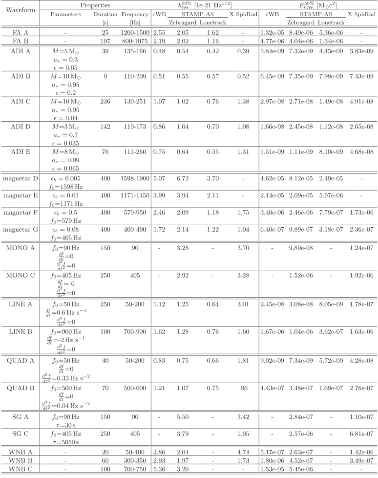
The sensitivity of each pipeline is estimated using 22 different types of simulated GW signals. Half of these are based on astrophysical source models and can be divided into 3 families: fallback accretion onto neutron stars (FA), black hole accretion disk instabilities (ADI) and magnetars. The other waveforms have ad-hoc mor-phologies that encapsulate the main characteristics for long-duration transients. The next section briefly de-scribes the models of sources whose chosen parameters are given in table I.
A. Waveform descriptions
FA: The fallback accretion disk model [17] focuses on newly born spinning neutron stars. In some unstable configurations, a non-axisymmetric deformation appears causing the production of GWs. The signal lasts from ∼ 10 s up to a few 100 s and its frequency evolution is almost linear.
ADI: This family includes five waveforms already con-sidered and described in the LIGO S5/S6 search [27] and the O1 GRB search [47]. In this model [19, 20], a thick accretion disk is coupled to a Kerr black hole through strong magnetic fields. This coupling is thought to gen-erate turbulence in the accretion torus that may form clumps of matter. The quadrupole components of the disk lead to gravitational wave emission that spin down the black hole and separate the clumps. The anti-chirp like waveform (frequency and amplitude decreases over time) depends on the mass of the central black hole M , the Kerr spin parameter a∗, and the fraction ǫ of the disk
mass that forms clumps.
Magnetar: Magnetic deformation of a rapidly rotat-ing neutron star can generate long-lastrotat-ing GWs that can live up to one hour with a slowly decreasing frequency and amplitude (i.e., an anti-chirp). We used the model described in [48], which includes two parameters: the magnetic ellipticity ǫb and the spin frequency f0 of the
neutron star, that entirely describe the frequency and amplitude variations.
Ad-hoc waveforms: These include monochromatic waveforms (MONO) and waveforms with a linear (LINE) and quadratic (QUAD) frequency evolution, as well as white noise band-limited (WNB) and sine-Gaussian bursts (SG) [27]. All of these waveforms have duration from ∼ 10 s up to a few 100 s and frequencies spanning the analysis range.
B. Detection efficiencies
In order to determine the detection efficiencies, wave-forms have been added coherently to the detector data at randomly chosen times over the full run period. We are using waveforms (H+ and H× polarizations) that have
been generated in the frame of the source. For each chosen time we draw a source sky position such that the whole set of source positions is uniformly distributed over the sky. In the frame of the detector the waveforms are elliptically polarized with an ellipticity that varies uni-formally between 0 and 1. The waveform amplitudes are also varied in order to estimate the dependency of the efficiency on the strength of the signal at a given FAR. Efficiency is simply the fraction of signals that are detected with a ranking statistic equal or larger than a value corresponding to the given FAR. To measure the in-trinsic amplitude strength of a waveform, we use the root-sum-square strain amplitude at the Earth hrss defined as
in [27], hrss= Z ∞ −∞ (H2 +(t) + H 2 ×(t)) dt, (1)
where H+ and H× are the GW strain polarizations in
the source frame. Table I provides the values of hrss at
which each pipeline recovers 50% or fewer of the injected signals for a FAR of 1 event in 50 years. Generally, cWB, Zebragard and X-SphRad have similar sensitivities while Lonetrack is better by a factor 2 for the waveforms that are well fit by B´ezier curves (LINE and QUAD).
Some of the listed waveforms are not detectable by a given pipeline. This is naturally the case for > 1 kHz signals for X-SphRad. But this is also the case for mono-chromatic signals (MONO and SG) for cWB and Lonet-rack. The reasons are different for each pipeline. For example, the way the pipelines whiten the data or es-timate the detector noise power spectrum may wash out continuous signals. This is the case for cWB and to a lesser extent for Zebragard and X-SphRad. Lonetrack by construction has no sensitivity to monochromatic signals and band limited white noise as these types of waveforms are not modelled by a Bezier curve.
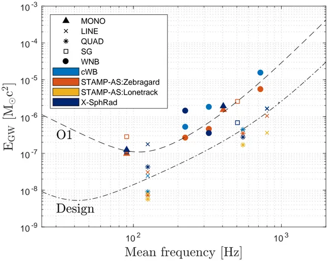
Figure 1 displays the GW energy emitted by a source located at 10 kpc for which the search efficiency drops below 50% for a FAR of 1 event in 50 years. The energy provides a universal quantity that can be directly com-pared to astrophysical predictions of the different possible sources. Assuming an isotropic GW emission, the energy emitted by a source at a distance r is given by
EGW = c3r2 4G Z ∞ −∞ h ˙h2++ ˙h 2 ×i dt, (2)
where ˙h+ and ˙h× are the time derivative of the GW
strain for the two polarizations in the detector frame. For the sake of visibility, only ad-hoc model waveforms are considered in the figure while values for all waveforms are reported in Table I. It illustrates the dependence on
the signal frequency which roughly follows the detect-ors’ sensitivity. Yet, one also sees that monochromatic (MONO and SG) and band limited white noise (WNB) waveform detections are systematically less efficient than the other waveforms. The minimal GW energy emit-ted by a source detecemit-ted in the Galaxy (10 kpc) is of the order of a few 10−8M
⊙c2. If one now looks at each
pipeline’s performance, for a given type of source, the detectable GW energy is spread over almost one order of magnitude and the most sensitive pipeline is different for each source.
To project the search sensitivity forward to the Ad-vanced LIGO detectors design sensitivity, we have con-sidered the matched filtered search results for an idealized monochromatic signal with a detection SNR threshold of 8. We are using monochromatic signals because the fre-quency is well defined. Results are then rescaled with a single factor such that the “O1” curve approximat-ively matches the MONO results of the O1 search. The “Design” curve is obtained using the predicted design Ad-vanced LIGO high-power signal recycling zero-detuning sensitivity curves [49], rescaled using the same factor as the “O1” curve. These curves show how the sensitiv-ity to monochromatic signals will evolve through the fu-ture observing runs assuming a FAR of 1 event in 50 years. In particular, a gain of two orders of magnitude on the energy is expected at low frequency with the Ad-vanced LIGO design sensitivity. Similar trends for the other waveforms are expected.
V. SEARCH RESULTS
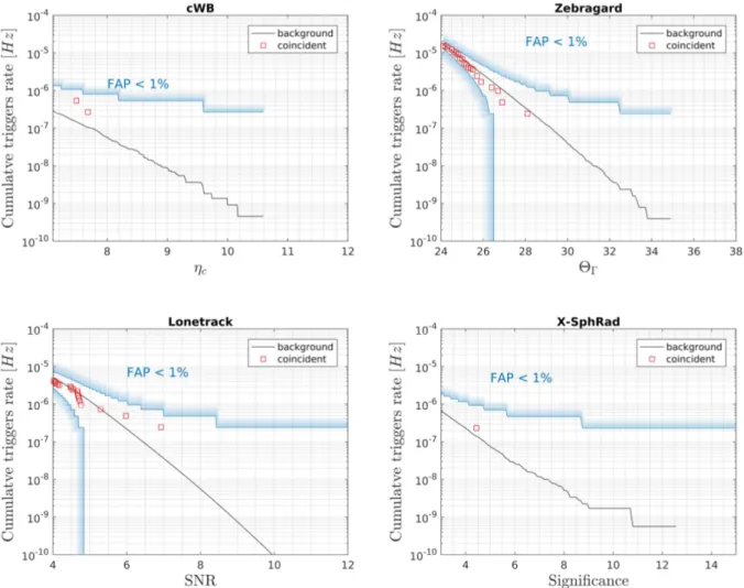
Figure 2 shows the distributions of the cumulative rate of coincident data triggers for each pipeline; these are ranked according to the pipelines’ detection statistic and are shown together with the estimated background. The X-SphRad and cWB distributions contain fewer triggers than the Zebragard or Lonetrack distributions because of the selection criteria that remove many low significant triggers at early stages. No significant excess of coin-cident triggers is found by any pipeline. The properties of the most significant triggers from each pipeline are reported in Table II. They are all compatible with the O1 background expectations as underlined by the rather large values of their false alarm probabilities (FAP). The FAP is the probability of observing at least one back-ground trigger with a ranking statistic larger than a given threshold.
Given the absence of long-duration transient GWs in the O1 data, we have updated the limits established in [27]. Assuming a Poissonian distribution of long-duration GW sources, we compute the 90% confidence level limit of the trigger rate using the loudest event stat-istic method [50], where systematic uncertainty coming from the strain amplitude calibration is folded into the upper limit calculation as in [27]. During the O1 science run, the amplitude calibration uncertainty was measured
to be 6% and 17% for the H1 and L1 detectors, respect-ively, in the 24–2048 Hz frequency band [47].
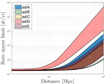
Figure 3 shows the rate upper limit as a function of distance for the ADI signals. The area is defined by the most and the least performing pipelines. The exclusion rate at short distance is limited by the observational dur-ation. Since O1 is shorter than S5 or S6, the event rate is less constrained. Conversely, the maximal distance for which one can expect to detect an event is improved by a factor ∼ 3.
Distances at which we can detect a signal with 50% efficiency are compared for all astrophysical waveforms in Table III. As already seen, detection distances for the 5 ADI waveforms are between 10 – 60 Mpc. On the other hand, the chance of detecting GWs from a magnetar or from the accretion of a black hole is limited to sources in the Local Group.
The fact that we do not see any signals in O1 is not un-expected. First, O1 is a short run, with only49 days of total coincident data, which is enough to detect multiple coalescences of binary black holes but quite short to de-tect long-duration GW signals considering the large un-certainties or unknowns about the rates of each of the potential long transient GW sources. Next, the energy of a long-duration signal is spread over a large number of pixels, which causes a decrease in the sensitivity of the pipelines. This explains why the short transient O1 search [12] is roughly an order of magnitude more sens-itive at a given frequency. Nevertheless, when compared to the S5/S6 results [27], the O1 long-duration transient search is better by a factor ∼ 10 due to the improvements in detector sensitivities.
VI. CONCLUSION
This paper reports the results of an all-sky search for unmodeled long-duration transient GWs in the first Advanced LIGO observing run. The parameter space covered by this search has been increased compared to the preceding search. Four different pipelines have searched for GW signals to efficiently cover the large space of possible waveforms. The most significant triggers found by each pipeline are consistent with the noise background, excluding for now a long duration GW transient detection.
Upper limits have been set on the rate of events for three families of long-duration GW transients (fallback accretion on neutron stars, black hole accretion disk in-stabilities and magnetar giant flares). They indicate we are sensitive to potential sources in the Local Group. Al-ternatively, if we consider a source in the Galaxy (10 kpc) we are sensitive to sources emitting at least 6×10⁻⁹M
⊙c2
for frequencies where the detectors’ sensitivities are max-imal. This is a lower bound (our results are spread over almost two orders of magnitude) but this is still an inter-esting achievement as it addresses an energy range that
Waveform Properties h 50% rss [1e-21 Hz1/2] E 50% GW [M⊙c 2 ]
Parameters Duration Frequency cWB STAMP-AS X-SphRad cWB STAMP-AS X-SphRad [s] [Hz] Zebragard Lonetrack Zebragard Lonetrack
FA A - 25 1200-1500 2.55 2.05 1.62 - 1.32e-05 8.49e-06 5.36e-06 -FA B - 197 800-1075 2.19 2.02 1.16 - 4.77e-06 4.04e-06 1.34e-06 -ADI A M=5 M⊙ 39 135-166 0.48 0.54 0.42 0.39 5.84e-09 7.32e-09 4.43e-09 3.83e-09
a∗= 0.3 ǫ= 0.05
ADI B M=10 M⊙ 9 110-209 0.51 0.55 0.57 0.52 6.45e-09 7.35e-09 7.98e-09 7.43e-09 a∗= 0.95
ǫ= 0.2
ADI C M=10 M⊙ 236 130-251 1.07 1.02 0.76 1.38 2.97e-08 2.71e-08 1.49e-08 4.91e-08 a∗= 0.95
ǫ= 0.04
ADI D M=3 M⊙ 142 119-173 0.86 1.04 0.70 1.08 1.66e-08 2.45e-08 1.12e-08 2.65e-08 a∗= 0.7
ǫ= 0.035
ADI E M=8 M⊙ 76 111-260 0.75 0.64 0.55 1.31 1.51e-09 1.11e-09 8.10e-09 4.68e-08 a∗= 0.99
ǫ= 0.065
magnetar D ǫb= 0.005 400 1598-1900 5.07 6.72 3.70 - 4.62e-05 8.12e-05 2.49e-05 -f0=1598 Hz
magnetar E ǫb= 0.01 400 1171-1450 3.99 3.94 2.11 - 2.14e-05 2.09e-05 5.97e-06 -f0=1171 Hz
magnetar F ǫb= 0.5 400 579-950 2.46 2.09 1.18 1.75 3.40e-06 2.46e-06 7.79e-07 1.73e-06 f0=579 Hz
magnetar G ǫb= 0.08 400 400-490 1.72 2.14 1.22 1.04 6.40e-07 9.89e-07 3.18e-07 2.36e-07 f0=405 Hz
MONO A f0=90 Hz 150 90 - 3.28 - 3.70 - 9.80e-08 - 1.24e-07 df
dt=0 d2f
dt2=0
MONO C f0=405 Hz 250 405 - 2.92 - 3.28 - 1.52e-06 - 1.92e-06 df
dt= 0 d2f
dt2=0
LINE A f0=50 Hz 250 50-200 1.12 1.25 0.64 3.01 2.45e-08 3.08e-08 8.05e-09 1.78e-07 df
dt=0.6 Hz s −1 d2f
dt2=0
LINE B f0=900 Hz 100 700-900 1.62 1.28 0.76 1.60 1.67e-06 1.04e-06 3.62e-07 1.63e-06 df
dt=-2 Hz s −1 d2f
dt2=0
QUAD A f0=50 Hz 30 50-200 0.83 0.75 0.66 1.81 9.02e-09 7.34e-09 5.72e-09 4.28e-08 df
dt=0 d2f
dt2=0.33 Hz s
−2
QUAD B f0=500 Hz 70 500-600 1.21 1.07 0.75 .96 4.43e-07 3.48e-07 1.69e-07 2.76e-07 df dt=0 d2f dt2=0.04 Hz s −2 SG A f0=90 Hz 150 90 - 5.50 - 3.42 - 2.84e-07 - 1.10e-07 τ=30 s SG C f0=405 Hz 250 405 - 3.79 - 1.95 - 2.57e-06 - 6.81e-07 τ=5050 s
WNB A - 20 50-400 2.86 2.04 - 4.74 5.17e-07 2.63e-07 - 1.42e-06 WNB B - 60 300-350 2.93 1.97 - 1.73 1.80e-06 4.52e-07 - 3.49e-07 WNB C - 100 700-750 5.36 3.20 - - 1.53e-05 5.45e-06 - -Table I. Search sensitivity of the four pipelines to the 22 waveform families used to cover the unmodeled long transient parameter space. The hrssat 50% efficiency is computed for a FAR of 1 event in 50 years. E50%GW is the GW energy emitted by a source located at 10 kpc for which the search efficiency drops below 50% for a FAR of 1 event in 50 years. The models are not sequentially named to avoid confusion with models used in former studies. The second column provides the parameters of the waveforms as defined in section IV A or in [27].
10
210
310
-910
-810
-710
-610
-510
-410
-3 MONO LINE QUAD SG WNB cWB STAMP-AS:Zebragard STAMP-AS:Lonetrack X-SphRadFigure 1. Emitted GW energy versus frequency for sources located at 10 kpc detected with 50% efficiency and a FAR of 1 event in 50 years. Results are shown for all the ad-hoc waveforms. The “O1” and “Design” curves are obtained with a monochromatic signal single template matched filtering search using the measured O1 and the predicted high-power signal recycling zero-detuning Advanced LIGO [49] sensitivity curves respectively. Both curves are rescaled so that the curve “O1” matches the MONO results of this search.
is astrophysically relevant [51, 52]. New data have been acquired recently by the LIGO detectors (observing run O2) with a sensitivity similar to O1 and a longer ob-servation time which increases the chance of observing a long-duration transient GW source [53]. The Advanced Virgo detector has joined for the first time the advanced GW detector network on August 1st 2017; this increases
sky coverage and improves the prospects for detection. In a few years, Advanced LIGO and Advanced Virgo should reach their design sensitivities. We have shown that we should gain between one and two orders of magnitude, depending on the frequency range, in the sensitivity to detect GW energy as low as ∼ 10−8 M
⊙c2 for a source
emitting a monochromatic signal at ∼ 90 Hz and located at 10 [kpc].
ACKNOWLEDGMENTS
The authors gratefully acknowledge the support of the United States National Science Foundation (NSF) for the construction and operation of the LIGO Laboratory and Advanced LIGO as well as the Science and Tech-nology Facilities Council (STFC) of the United King-dom, the Max-Planck-Society (MPS), and the State of Niedersachsen/Germany for support of the construction of Advanced LIGO and construction and operation of the GEO600 detector. Additional support for Advanced LIGO was provided by the Australian Research Council. The authors gratefully acknowledge the Italian Istituto Nazionale di Fisica Nucleare (INFN), the French Centre National de la Recherche Scientifique (CNRS) and the Foundation for Fundamental Research on Matter sup-ported by the Netherlands Organisation for Scientific Re-search, for the construction and operation of the Virgo detector and the creation and support of the EGO
consor-Figure 2. Cumulative trigger rate as function of the triggers’ ranking statistic for the four pipelines. The coincident triggers are represented by the red squares while the black curves show the estimation of the contribution of the accidental coincident noise triggers. The blue isocurves indicate the trigger rate that corresponds to a false alarm probability (FAP) lower than 1%. This illustrates that all coincident triggers’ distributions are compatible with the expected background. For cWB and X-SphRad the lower isocurve is not displayed because it falls outside of the axis limits.
tium. The authors also gratefully acknowledge research support from these agencies as well as by the Council of Scientific and Industrial Research of India, the Depart-ment of Science and Technology, India, the Science & En-gineering Research Board (SERB), India, the Ministry of Human Resource Development, India, the Spanish Agen-cia Estatal de Investigaci´on, the Vicepresid`enAgen-cia i Consel-leria d’Innovaci´o, Recerca i Turisme and the Conselleria d’Educaci´o i Universitat del Govern de les Illes Balears, the Conselleria d’Educaci´o, Investigaci´o, Cultura i Es-port de la Generalitat Valenciana, the National Science Centre of Poland, the Swiss National Science Foundation (SNSF), the Russian Foundation for Basic Research, the Russian Science Foundation, the European Commission, the European Regional Development Funds (ERDF), the Royal Society, the Scottish Funding Council, the Scot-tish Universities Physics Alliance, the Hungarian Sci-entific Research Fund (OTKA), the Lyon Institute of
Ori-gins (LIO), the Paris ˆIle-de-France Region, the National Research, Development and Innovation Office Hungary (NKFI), the National Research Foundation of Korea, Industry Canada and the Province of Ontario through the Ministry of Economic Development and Innovation, the Natural Science and Engineering Research Council Canada, the Canadian Institute for Advanced Research, the Brazilian Ministry of Science, Technology, Innova-tions, and CommunicaInnova-tions, the International Center for Theoretical Physics South American Institute for Fun-damental Research (ICTP-SAIFR), the Research Grants Council of Hong Kong, the National Natural Science Foundation of China (NSFC), the Leverhulme Trust, the Research Corporation, the Ministry of Science and Tech-nology (MOST), Taiwan and the Kavli Foundation. The authors gratefully acknowledge the support of the NSF, STFC, MPS, INFN, CNRS and the State of Niedersach-sen/Germany for provision of computational resources.
Pipeline Ranking FAP Frequency Duration GPS time statistic [Hz] [s] cWB ηc= 7.6 0.33 2039-2041 5.5 1132990790 Zebragard ΘΓ= 28.2 0.72 1034-1120 51 1131758576 Lonetrack SNR = 6.95 0.36 85-1549 208 1136368706 X-SphRad Significance = 4.5 0.44 895-909 4 1135861536
Table II. Properties of the most significant coincident triggers found by each of the long transient search pipelines during the O1 observational run. FAP is the probability of observing at least 1 noise trigger more significant that the most significant coincident trigger.
Figure 3. Upper limits at 90% confidence on the rate of GW events from accretion disk instability as a function of the dis-tance. The band covers the results from the best and the worst pipelines for each tested waveforms. O1 amplitude cal-ibration errors are accounted for in the upper limits calcula-tion.
[1] B. P. Abbott et al. (LIGO Scientific Collaboration and Virgo Collaboration), Phys. Rev. Lett. 116, 061102 (2016), 1602.03837.
[2] B. P. Abbott et al. (LIGO Scientific Collaboration and Virgo Collaboration), Phys. Rev. Lett. 116, 241103 (2016), 1606.04855.
[3] B. P. Abbott et al. (LIGO Scientific Collaboration and Virgo Collaboration), Phys. Rev. X 6, 041015 (2016), 1606.04856.
[4] B. P. Abbott et al. (LIGO Scientific Collaboration and Virgo Collaboration), Phys. Rev. D 93, 122004 (2016), 1602.03843.
[5] B. P. Abbott et al. (LIGO Scientific Collaboration and Virgo Collaboration), Phys. Rev. D 93, 122003 (2016),
1602.03839.
[6] B. P. Abbott et al. (LIGO Scientific Collaboration and Virgo Collaboration), Phys. Rev. Lett. 118, 221101 (2017), 1706.01812.
[7] B. P. Abbott et al. (LIGO Scientific Collaboration and Virgo Collaboration), Phys. Rev. Lett. 119, 141101 (2017), 1709.09660.
[8] B. P. Abbott et al. (LIGO Scientific Collaboration and Virgo Collaboration), Phys. Rev. Lett. 119, 161101 (2017), 1710.05832.
[9] B. P. Abbott et al. (LIGO Scientific Collaboration, Virgo Collaboration, Fermi-GBM, INTEGRAL), Astrophys. J. 848, L13 (2017), 1710.05834.
Waveform Distance50% [Mpc] cWB STAMP-AS X-SphRad Zebragard Lonetrack FA A 1.08 1.34 1.69 -FA B 1.76 1.91 3.32 -ADI A 19.1 17.1 22.0 23.6 ADI B 58.3 54.6 52.5 54.4 ADI C 29.1 30.5 41.1 22.6 ADI D 10.1 8.33 12.3 8.02 ADI E 33.6 39.2 46.0 19.1 magnetar D 0.14 0.11 0.19 -magnetar E 0.20 0.20 0.37 -magnetar F 0.50 0.57 1.02 0.68 magnetar G 0.43 0.35 0.61 0.71 Table III. Distances at which the pipeline efficiency drops be-low 50% for a FAR of 1 event in 50 years for the accretion disk instability, magnetar and fallback accretion signals considered in the O1 search.
DFN, INTEGRAL, Virgo, Insight-Hxmt, MAXI Team, Fermi-LAT, J-GEM, RATIR, IceCube, CAASTRO, LWA, ePESSTO, GRAWITA, RIMAS, SKA South Africa/MeerKAT, H.E.S.S., 1M2H Team, IKI-GW Follow-up, Fermi GBM, Pi of Sky, DWF (Deeper Wider Faster Program), Dark Energy Survey, MAS-TER, AstroSat Cadmium Zinc Telluride Imager Team, Swift, Pierre Auger, ASKAP, VINROUGE, JAG-WAR, Chandra Team at McGill University, TTU-NRAO, GROWTH, AGILE Team, MWA, ATCA, AST3, TOROS, Pan-STARRS, NuSTAR, ATLAS Tele-scopes, BOOTES, CaltechNRAO, LIGO Scientific, High Time Resolution Universe Survey, Nordic Optical Tele-scope, Las Cumbres Observatory Group, TZAC Con-sortium, LOFAR, IPN, DLT40, Texas Tech University, HAWC, ANTARES, KU, Dark Energy Camera GW-EM, CALET, Euro VLBI Team, ALMA), Astrophys. J. 848, L12 (2017), 1710.05833.
[11] B. P. Abbott et al. (LIGO Scientific Collaboration and Virgo Collaboration), Astrophys. J. 832, L21 (2016), 1607.07456.
[12] B. P. Abbott et al. (LIGO Scientific Collaboration and Virgo Collaboration), Phys. Rev. D 95, 042003 (2017), 1611.02972.
[13] B. P. Abbott et al. (LIGO Scientific Collaboration and Virgo Collaboration), Phys. Rev. D 96, 022001 (2017), 1704.04628.
[14] D. Lai and S. L. Shapiro, Astrophys. J. 442, 259 (1995), astro-ph/9408053.
[15] C. Cutler, Phys. Rev. D 66, 084025 (2002), gr-qc/0206051.
[16] A. L. Piro and C. D. Ott, Astrophys. J. 736, 108 (2011), 1104.0252.
[17] A. L. Piro and E. Thrane, Astrophys. J. 761, 63 (2012). [18] A. L. Piro and E. Pfahl, Astrophys. J. 658, 1173 (2007),
astro-ph/0610696.
[19] M. H. P. M. van Putten, Phys. Rev. Lett 87, 091101 (2001).
[20] M. H. P. M. van Putten, Astrophys. J. Lett. 684, L91 (2008).
[21] A. Corsi and P. M´esz´aros, Astrophys. J. 702, 1171 (2009).
[22] L. Gualtieri, R. Ciolfi, and V. Ferrari, Class. Quantum Grav. 28, 114014 (2011), 1011.2778. [23] B. D. Metzger, D. Giannios, T. A. Thompson, N.
Buc-ciantini, and E. Quataert, Mon. Not. Roy. Astron. Soc. 413, 2031 (2011), 1012.0001.
[24] A. Rowlinson, P. T. O’Brien, B. D. Metzger, N. R. Tan-vir, and A. J. Levan, Mon. Not. R. Astron. Soc. 430, 1061 (2013), 1301.0629.
[25] A. Marek, H. T. Janka, and E. Mueller, Astron. Astro-phys. 496, 475 (2009), 0808.4136.
[26] J. W. Murphy, C. D. Ott, and A. Burrows, Astrophys. J. 707, 1173 (2009), 0907.4762.
[27] B. P. Abbott et al. (LIGO Scientific Collaboration and Virgo Collaboration), Phys. Rev. D 93, 042005 (2016), 1511.04398.
[28] B. P. Abbott et al. (LIGO Scientific Collaboration and Virgo Collaboration), Class. Quant. Grav. 33, 134001 (2016), 1602.03844.
[29] N. Christensen (LIGO Scientific Collaboration and Virgo Collaboration), Class. Quantum Grav. 27, 194010 (2010).
[30] J. Aasi et al. (LIGO Scientific Collaboration and Virgo Collaboration), Class. Quantum Grav. 32, 115012 (2015), 1410.7764.
[31] M. Was, M.-A. Bizouard, V. Brisson, F. Cavalier, M. Davier, P. Hello, N. Leroy, F. Robinet, and M. Va-voulidis, Classical and Quantum Gravity 27, 015005 (2010).
[32] S. Klimenko et al., Phys. Rev. D 93, 042004 (2016), 1511.05999.
[33] T. Prestegard, Thesis, University of Minnesota (2016). [34] T. Isogai, the Ligo Scientific Collaboration, and the
Virgo Collaboration, Journal of Physics: Conference Series 243, 012005 (2010).
[35] G. Farin, Curves and Surfaces for CAGD, Fourth
Edi-tion: A Practical Guide (Academic Press, 1996).
[36] E. Thrane and M. Coughlin, Phys. Rev. D 88, 083010 (2013), 1308.5292.
[37] E. Thrane and M. Coughlin, Phys. Rev. D 89, 063012 (2014), 1401.8060.
[38] M. Coughlin, P. Meyers, S. Kandhasamy, E. Thrane, and N. Christensen, Phys. Rev. D 92, 043007 (2015), 1505.00205.
[39] E. Thrane and M. Coughlin, Phys. Rev. Lett. 115, 181102 (2015), 1507.00537.
[40] M. Coughlin, E. Thrane, and N. Christensen, Phys. Rev. D 90, 083005 (2014), 1408.0840.
[41] M. Coughlin, P. Meyers, E. Thrane, J. Luo, and N. Christensen, Phys. Rev. D 91, 063004 (2015), 1412.4665.
[42] K. C. Cannon, Phys. Rev. D 75, 123003 (2007). [43] M. Edwards, Thesis, University of Cardiff (2013). [44] P. J. Sutton et al., New J. Phys. 12, 053034 (2010),
0908.3665.
[45] M. Was, P. J. Sutton, G. Jones, and I. Leonor, Phys. Rev. D 86, 022003 (2012), 1201.5599.
[46] M. Edwards and P. J. Sutton, J. Phys. Conf. Ser. 363, 012025 (2012).
[47] B. P. Abbott et al. (LIGO Scientific Collaboration) (2016), 1602.03845.
[48] S. Dall’Osso, B. Giacomazzo, R. Perna, and L. Stella, Astrophys. J. 798, 25 (2015).
[49] D. Shoemaker (LIGO Scientific Collaboration), Advanced
ligo anticipated sensitivity curves (2009), lIGO DCC,
URL https://dcc.ligo.org/LIGO-T0900288/public. [50] P. R. Brady, J. D. Creighton, and A. G. Wiseman,
Class. Quantum Grav. 21, S1775 (2004), gr-qc/0405044. [51] R. Turolla, S. Zane, and A. Watts, Rept. Prog. Phys. 78,
116901 (2015), 1507.02924.
[52] E. Mueller, M. Rampp, R. Buras, H.-T. Janka, and D. H. Shoemaker, Astrophys. J. 603, 221 (2004), astro-ph/0309833.
[53] J. Aasi et al. (LIGO Scientific Collaboration and Virgo Collaboration), Living Rev. Rel. 19 (2016), liv-ing Rev. Rel. 19, 1 (2016), 1304.0670.
![[1] Denti E., Di Rito G., Galatolo R., Comandi di volo Fly-By-Wire:](data:image/gif;base64,R0lGODlhAQABAIAAAP///wAAACH5BAEAAAAALAAAAAABAAEAAAICRAEAOw==)