Innovative model updating procedure for dynamic identification and damage assessment of structures

(1)

A

l

m

a

M

a

t

e

r

S

t

u

d

i

o

r

u

m

–

U

n

i

v

e

r

s

i

t

à

d

i

B

o

l

o

g

n

a

DOTTORATO DI RICERCA IN

INGEGNERIA CIVILE, CHIMICA, AMBIENTALE E DEI

MATERIALI

Ciclo XXX

Settore Concorsuale: 08/B3

Settore Scientifico Disciplinare: ICAR/09

INNOVATIVE MODEL UPDATING PROCEDURE FOR DYNAMIC

IDENTIFICATION AND DAMAGE ASSESSMENT OF STRUCTURES

Presentata da:

MICHELE TONDI

Coordinatore Dottorato

Supervisore

Prof. Luca Vittuari

Prof. Marco Savoia

Co-Supervisore

Dott. Marco Bovo

(2)

(3)

I

ACKNOWLEDGEMENTS

During my Ph.D., several people helped me and deserve my acknowledgement. First of all my parents Leonardo and Doriana, their sustain and kindness helped me to finish the Ph.D.. My grandparents Maddalena, Marisa and Silvano, they supported me for my whole life. I wish to thank Giulia for all the things who made during my Ph.D., especially when I was abroad. I very important acknowledge goes to Marco Bovo who helped me for the three years of Ph.D. with a helpful advices and ideas. Thanks to Professor Marco Savoia, one of the best professor and engineer I have never met, he gave me several and helpful advices. Thanks to Loris Vincenzi, he helped me in a very important way. Thanks also to Professor Claudio Mazzotti, his advices were very useful for my research activities. A very important appreciation goes to Sina, Hadi and Amir; without them my staying in Buffalo would have been horrible. Another very important appreciation go to Professor Stavridis, he helped me with my research more than he thinks. I wish to thank Professor Moaveni, I have never met him personally but his advices helped me in a very important way. I want to thank Michele Naldi, I appreciated our conversations and friendship. I want to thank all my friends of Castel d'Aiano and Montese, thank you for the fun, laughs and the wonderful evenings spent together.

(8)

(9)

VII

LIST OF TABLES

Table 1.1: Relations proposed in literature for the calculation of w/d ratio (Tarque et al.,

2015). ...15

Table 2.1: Standard deviations and CoVs of parameters from uncertainties evaluation and Monte Carlo realizations. ...53

Table 4.1: Reference values of parameters. ...95

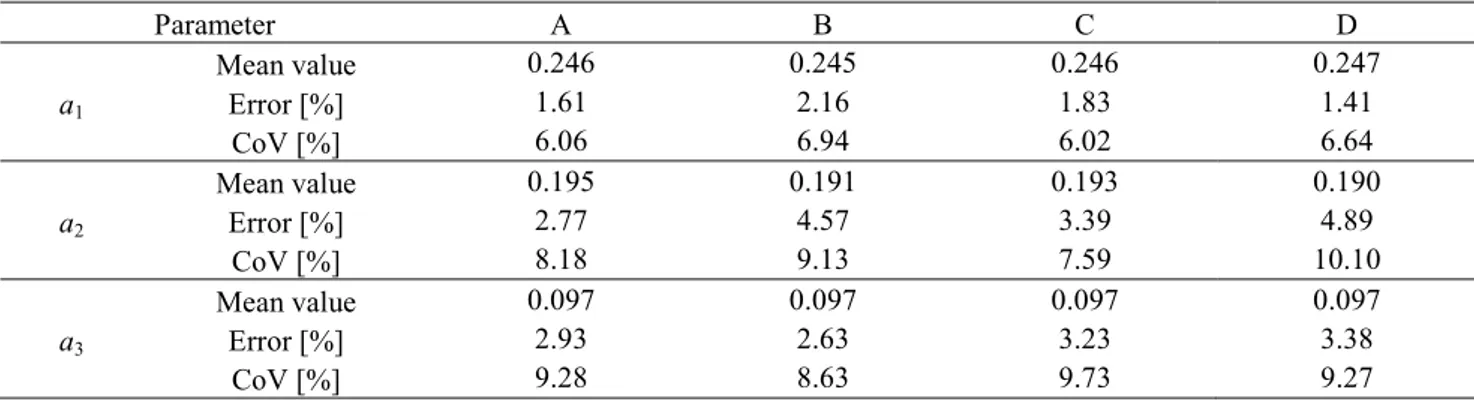
Table 4.2: Mean values, errors and CoVs of parameters for 2-D sample. ...95

Table 4.3: Reference values of the equivalent strut widths. ...95

Table 4.4: Mean values, errors and CoVs for case AA-0-0, AS-0-0 and AAv-0-0. ...95

Table 4.5: Mean values, errors and CoVs for case AA-1-I, AA-2-I and AA-3-I. ...96

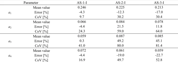
Table 4.6: Mean values, errors and CoVs for case AS-1-I, AS-2-I and AS-3-I. ...96

Table 4.7: Mean values, errors and CoVs for case AA-2-I, AA-2-II and AA-2-III. ...96

Table 4.8: Mean values, errors and CoVs for case AAv-2-I, AAv-2-II and AAv-2-III. ...97

Table 4.9: Mean values, errors and CoVs for case AA-2-I with DE-Q and two steps procedures. ...97

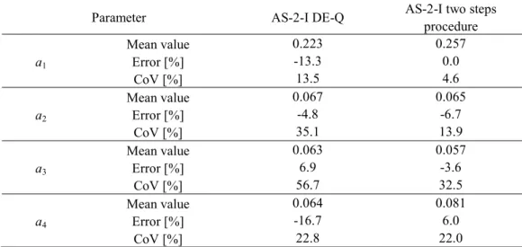
Table 4.10: Mean values, errors and CoVs for case AS-2-I with DE-Q and two steps procedures. ...97

Table 4.11: Mean values, errors and CoVs for case AA-2-I with and without determinant equations using two steps procedure (for the system without determinant equations only the first step is needed).. ...98

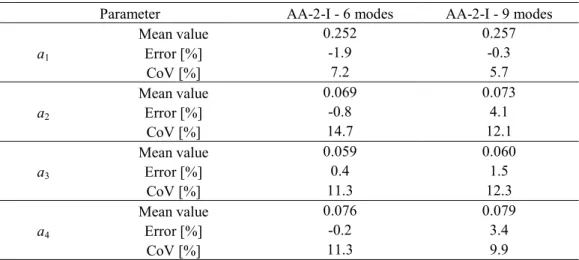
Table 4.12: Mean values, errors and CoVs for case AA-2-I with 6 and 9 modes. ...98

Table 4.13: Chi-square tests for cases AA-2-I and AS-2-I. ...99

Table 4.14: Statistical distributions of parameters for cases AA-2-I and AS-2-I. ...99

Table 5.1: Dynamic tests performed in the specimen (from Moaveni et al,2013). ...125

Table 5.2: Identified frequencies from white noise tests. ...125

Table 5.3: Comparison between experimental and numerical frequencies and MAC values. ...126

Table 5.4: Walls demolition sequence and resulted damage state. ...126

Table 5.5: Summary of system identification results (Yousefianmoghadam et al., 2015). ...126

Table 5.6: Comparison between modes components and re-built modes components. ...126

Table 5.7: Values of parameters for 4 parameters case. ...126

Table 5.8: Comparison between experimental and numerical frequencies and MAC values for 4 parameters case. ...127

(10)

VIII

Table 5.9: Damage parameters for 4 parameters case. ...127

Table 5.10: Mean values, standard deviations and CoVs for experimental frequencies. ...127

Table 5.11: Mean values, standard deviations and CoV values of parameters. ...128

Table 5.12: Mean values, standard deviations, CoVs and errors for frequencies and MAC values...128

Table 5.13: Values of parameters for 8 parameters case. ...128

Table 5.14: Comparison between experimental and numerical frequencies and MAC values for 8 parameters case. ...129

Table 5.15: Damage parameters for 8 parameters case. ...129

Table 5.16: Comparison between experimental and numerical frequencies and MAC values for 8 parameters case without updating the ground storey parameters for DS2, DS3 and DS4. ...129

Table 7.1: Modes components chosen for the procedure. ...171

Table 7.2: w/d values for the 3 parameters - Case 1. ...171

Table 7.3: Frequencies before and after retrofitting - Case 1. ...171

Table 7.4: Modified modes components chosen for the procedure. ...172

Table 7.5: w/d values for the 3 parameters - Case 2. ...172

Table 7.6: Frequencies before and after retrofitting - Case 2. ...172

Table A.1: Mean values, variances, standard deviations and CoVs of parameter from distribution propagation and Monte Carlo procedure. ...185

Table B.1: CoVs of parameters changing the number of parameters updated. ...193

Table C.1: Mean values, variances, standard deviations and CoVs of parameter from uncertainties evaluation and Monte Carlo procedure. ...199

(11)

IX

LIST OF FIGURES

Figure 1.1: Algorithm scheme for DE method (Vincenzi and Savoia, 2010). ...17

Figure 1.2: Mutation process by random combination (Vincenzi and Savoia, 2010). ...17

Figure 1.3: Flowchart of the DE-Q algorithm(Vincenzi and Savoia, 2015). ...18

Figure 1.4: Approximation of cost function by quadratic response surface. (Vincenzi and Savoia, 2010). ...18

Figure 2.1: Two bays three storey infilled frame decomposition with two parameters. ...55

Figure 2.2: Flowchart of the two steps algorithm. ...55

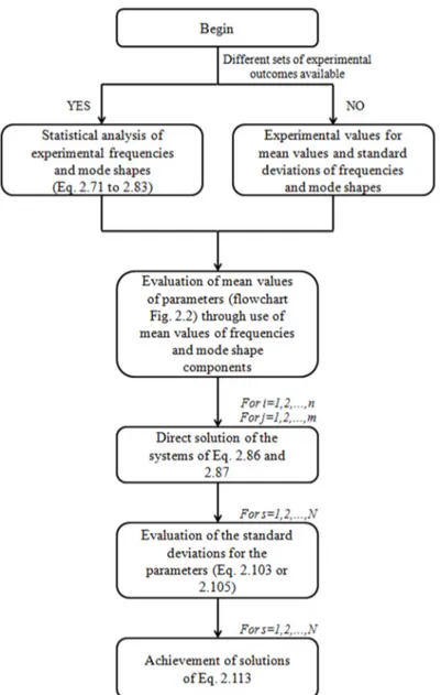
Figure 2.3: Flowchart of the two steps algorithm with uncertainties evaluation. ...56

Figure 2.4: Flowchart of the two steps algorithm for complete statistical analysis of the procedure. ...57

Figure 2.5: Frequencies histograms of parameters a1, a2 from Monte Carlo analysis. ...58

Figure 2.6: Flowchart of the algorithm with DE-Q procedure. ...58

Figure 2.7: Flowchart of the algorithm with DE-Q procedure and uncertainties evaluation. ...59

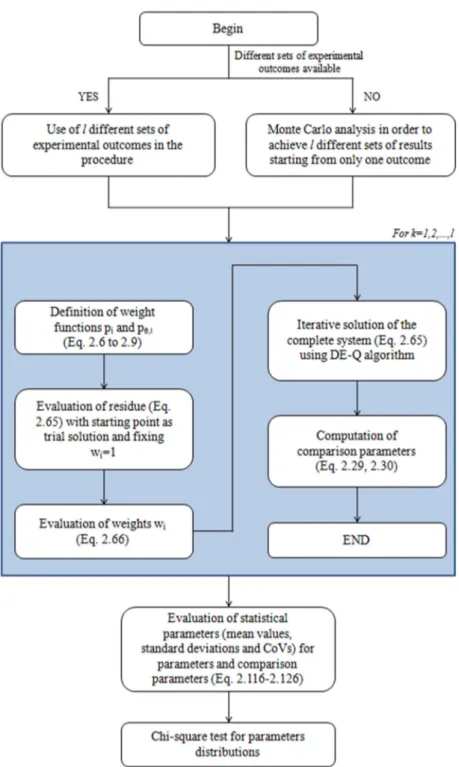
Figure 2.8: Flowchart of the algorithm with DE-Q procedure for complete statistical analysis. ...60

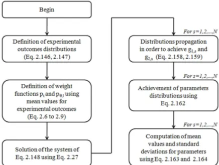
Figure 2.9: Flowchart of the algorithm for the direct statistical distribution analysis. ...61

Figure 3.1: General representation of rigid diaphragm components from l+p displacements. ...85

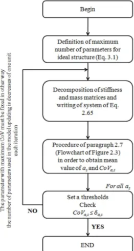
Figure 3.2: Flowchart of the procedure for obtaining of the maximum number of parameter in real structure. ...85

Figure 4.1: View of the 2-D sample structure. ...101

Figure 4.2: Parameters arrangement. ...101

Figure 4.3: Frequencies histograms of parameters a1, a2, a3 for 2-D sample - Case A. ...102

Figure 4.4: Frequencies histograms of parameters a1, a2, a3 for 2-D sample - Case B. ...102

Figure 4.5: Frequencies histograms of parameters a1, a2, a3 for 2-D sample - Case C. ...103

Figure 4.6: Frequencies histograms of parameters a1, a2, a3 for 2-D sample - Case D. ...104

Figure 4.7: Plan view of 3-D samples. ...104

Figure 4.8: Views of 3-D samples - Case AA: (a) North elevation, (b) West elevation, (c) South elevation, (d) East elevation. ...104

Figure 4.9: Views of 3-D samples - Case AS: (a) North elevation, (b) West elevation, (c) South elevation, (d) East elevation. ...105

Figure 4.10: Views of 3-D samples - Case AAv: (a) North elevation, (b) West elevation, (c) South elevation, (d) East elevation - The blue infill is the model error. ...105

(12)

X

Figure 4.11: Frequencies histograms of parameters a1, a2, a3, a4 for 3-D sample

- Case AA-2-I. ...106

Figure 4.12: Frequencies histograms of parameters a1, a2, a3, a4 for 3-D sample - Case AS-2-I. ...106

Figure 4.13: Frequencies histograms of parameters a1, a2, a3, a4 for 3-D sample - Case AAv-2-I. ...107

Figure 4.14: Frequencies histograms of parameters a1, a2, a3, a4 for 3-D sample - Case AA-2-I along with main fitted distributions: (a) parameter a1, (b) parameter a2, (c) parameter a3, (d) parameter a4. ...109

Figure 4.15: Frequencies histograms of parameters a1, a2, a3, a4 for 3-D sample - Case AS-2-I along with main fitted distributions: (a) parameter a1, (b) parameter a2, (c) parameter a3, (d) parameter a4. ...111

Figure 5.1: Plan view of the prototype structure (from Moaveni et al,2013). ...131

Figure 5.2: Elevation view of the prototype structure (from Moaveni et al,2013). ...131

Figure 5.3: Design of the tree storey specimen (dimensions in m) (from Stavridis et al, 2011). ...131

Figure 5.4: Cross sections of R.C. members (dimensions in mm) (from Stavridis et al, 2011). ....132

Figure 5.5: Front view of the specimen (from Moaveni et al, 2013). ...132

Figure 5.6: Location of accelerometers at each floor level (from Moaveni et al, 2013). ...132

Figure 5.7: Modes for damage state DS0: (a) Polar plot representation for complex mode shapes; (b) Vibration mode shapes (from Moaveni et al, 2013). ...132

Figure 5.8: Stick model representation. ...133

Figure 5.9: Parameters values for all damage states. ...133

Figure 5.10: Story stiffness for all damage states. ...133

Figure 5.11: Damage parameters for all damage states. ...134

Figure 5.12: Comparison between experimental and numerical mode shapes (the red lines are the experimental mode shapes, the blue lines are the numerical ones): (a) DS0; (b) DS1; (c) DS2; (d) DS3; (e) DS4; (f) DS5; (g) DS6; (h) DS7. ...135

Figure 5.13: Views of the structure under study: (a) north-west view; (b) north-east view (Song et al., 2017). ...135

Figure 5.14: First floor plan view with joists details (Yousefianmoghadam et al., 2015). ...136

Figure 5.15: Walls demolition sequence and resulted damage state (Yousefianmoghadam et al., 2015). ...136

(13)

XI

Figure 5.17: Mode shapes for roof level: (a) Mode 1; (b) Mode 2 (Yousefianmoghadam et al., 2015). ...137 Figure 5.18: Parameters definition for 4 parameters case: (a) Plan view of the first storey; (b) North

elevation, 1st parameter (in red); (c) East elevation, 2nd parameter (in orange); (d) South elevation, 3rd parameter (in green); (e) West elevation, 4th parameter (in

blue). ...138 Figure 5.19: Parameters values for all the damage states for 4 parameters case. ...139 Figure 5.20: Damage parameters for all the damage states for 4 parameters case. ...139 Figure 5.21: Comparison between parameters for undamaged structure and DS1 for 4 parameters case. ...140 Figure 5.22: Comparison between experimental and numerical mode shapes (the red lines are the

experimental mode shapes, the blue lines are the numerical ones): (a) DS1 - Mode 1; (b) DS1 - Mode 2; (c) DS2 - Mode 1; (d) DS2 - Mode 2; (e) DS3 - Mode 1;

(f) DS3 - Mode 2; (g) DS4 - Mode 1; (h) DS4 - Mode 2. ...144 Figure 5.23: Frequencies histograms of parameters a1, a2, a3 and a4 for damage state DS1. ...145 Figure 5.24: Mean values of parameters along with standard deviations for all the damage

states. ...145 Figure 5.25: Parameters definition for 8 parameters case: (a) Ground floor plan view; (b) First floor

plan view; (c) North elevation, 1st parameter in yellow, 5th parameter in red; (d) East elevation, 2nd parameter in black, 6th parameter in orange; (e) South elevation, 3rd parameter in violet, 7th parameter in green (f) West elevation, 4th parameter in dark blue, 8th parameter in blue. ...146 Figure 5.26: Parameters values for all the damage states for 8 parameters case. ...147 Figure 5.27: Damage parameters for all the damage states for 8 parameters case. ...147 Figure 5.28: Comparison between parameters for undamaged structure and DS1 for 8 parameters case. ...148 Figure 5.29: Damage parameters between undamaged structure and DS1 for 8 parameters

case. ...148 Figure 6.1: Flowchart of the two steps algorithm for unrelated non-linear parameters. ...159 Figure 6.2: Flowchart of the two steps algorithm with uncertainties evaluation for unrelated non-linear parameters. ...160 Figure 6.3: Flowchart of the two steps algorithm for complete statistical analysis for unrelated

(14)

XII

Figure 6.4: Flowchart of the algorithm with DE-Q procedure for related non-linear

parameters. ...162

Figure 6.5: Flowchart of the algorithm with DE-Q procedure and uncertainties evaluation for related non-linear parameters. ...162

Figure 6.6: Flowchart of the algorithm with DE-Q procedure for complete statistical analysis for related non-linear parameters. ...163

Figure 7.1: Flowchart of the procedure. ...173

Figure 7.2: Plan view of Case 1 (dimensions in cm). ...173

Figure 7.3: Elevation views of Case 1: (a) South elevation; (b) East elevation; (c) North elevation; (d) West elevation. ...174

Figure 7.4: Elevation views of Case 2: (a) South elevation; (b) East elevation; (c) North elevation; (d) West elevation. ...175

Figure 7.5: Flowchart of procedure for unrelated non-linear parameters. ...175

Figure 7.6: Flowchart of procedure for related non-linear parameters. ...176

Figure A.1: Analytical distribution along with calibrated Gaussian and Cauchy distributions. ....187

Figure A.2: Analytical distribution along with normalized frequencies histogram from Monte Carlo analysis. ...187

Figure C.1: View of the sample structure. ...201

Figure C.2: Target function H for not perturbed system. ...201

(15)

XIII

LIST OF ABBREVIATIONS

COMAC Coordinate MAC CoV Coefficient of Variation cov Covariance

CR Crossover Constant DE Differential Evolution DMU Direct Matrix Updating DOF Degree Of Freedom DS Damage State

ECM Eigendynamic Constraint Method EMM Error Matrix Method

EQ Earthquake base excitation

ERA Eigensystem Realization Algorithm FE Finite Elements

FMAC Frequency-scaled MAC FRF Frequency Response Function GRSM General Response Surface Method IES Inverse Eigensensitivity Method

LVDT Linear Variable Displacement Transducer IMAC Improved MAC

MAC Modal Assurance Criterion

(16)

XIV

NEES Network for Earthquake Engineering Simulation NExT Natural Excitation Technique

NCO Normalized MAC

NMD Normalized Modal Difference pdf Probability Density Function R.C. Reinforced Concrete

RFM Response Function Method RSM Response Surface Methodology UCSD University of California San Diego WN White Noise base excitation

(17)

XV

ABSTRACT

The model updating technique allows the understanding of the dynamic behavior of a system and its damage state. In the last years, the structural monitoring has increased its applicability thanks to the decrease of the cost of sensors and improvements in the computational power. More and more structures are today instrumented in order to assess the intervention of progressive damages, understand their structural behavior and safety in almost real time. Nowadays, the real time identification of structural parameters and damage assessment is no longer unachievable. Moreover, the uncertainties evaluation is another important task required by the model updating procedures. Combining real time assessment and uncertainties evaluation, the algorithms can drive to a judgment about unsafety conditions in the buildings, with possible evacuation and securing of the structures, which is more and more required to structural health monitoring systems.

The algorithms developed in this work are focused on these topics, especially on very quick model updating procedure, with uncertainties evaluation, which allows to estimate the structural parameters along with an error assessment. The quickness of the algorithm enables for its use in real time monitoring of actual structures. The algorithm itself is based on an innovative two steps procedure, with uncertainties evaluation, solving the inverse eigenvalues problem. The first step is achieved with closed form solution (without considering the determinant equations). If the solution does not satisfy the fixed thresholds, the second iterative step should be performed in order to improve the agreement between experimental outcomes and numerical ones. This procedure allows us to write the partial derivatives of the problem itself, with respect to the experimental outcomes, in closed form. Therefore, the parameters uncertainties are computed using the errors propagation. A second procedure is developed facing the complete problem entirely in iterative way, using a genetic algorithm with response surfaces (the so-called DE-Q algorithm). The uncertainties evaluation is done also for this procedure in closed form.

A sensitivity analysis has been performed on 2-D and 3-D infilled framed structures varying the perturbation values on frequencies and mode shapes and varying the parameters arrangement. Comparison between the two procedures has been done in terms of mean values and coefficients of variations of parameters. Another comparison has been performed in order to understand the influence of the determinant equations and the number of modes used.

Two real structures have been then analyzed with the algorithm, the first one is a three storey, two bays 2-D infilled frame tested with shake table in San Diego, CA, US, of which seven damage

(18)

XVI

states were achieved scaling accelerogram of actual earthquakes. The second one is a two storey, 3-D infilled framed structure located in El-Centro, CA, US, tested with ambient vibrations and forced vibrations through shaker. Four damage states were achieved artificially through infills removal at the first storey. For both the structures, a damage assessment has been achieved and, for the last one, a sensitivity analysis using several data windows for ambient vibrations is reported. Then, a generalization of the procedure in order to take into account the possibility of non-linear parameters is studied.

In the last part of this thesis, the algorithm is used in order to find a first trial solution for the retrofitting problem of existing structures. Two sample structures are analyzed and the comparison between numerical and expected parameters is performed. A generalization for non-linear parameters is then developed.

Keywords: Model Updating, Damage Assessment, Dynamic identification, Inverse Eigenvalues Problem, Statistical Analysis, Error Propagation, Infilled Frames, Stick Model, Ambient Vibrations, Sensitivity Analysis, Monte Carlo Procedure, Genetic Algorithm, Response Surfaces Methodology, Seismic Retrofitting, Modal Assurance Criterion, Shake Table Tests, Shaker, Matlab, OpenSEES.

(19)

XVII

SOMMARIO

La procedura di model updating è una tecnica alquanto datata che permette di comprendere il comportamento dinamico di un sistema e il suo stato di danno. Negli ultimo anni, il monitoraggio strutturale ha incrementato la sua applicabilità grazie al ridotto costo dei sensori e al miglioramento della potenza computazionale. Sempre più strutture sono oggi strumentate per valutare i loro danni e capire il comportamento dinamico stesso. La valutazione in tempo reale dei parametri strutturali e dello stato di danno è oggigiorno non più irraggiungibile. La valutazione delle incertezze sui parametri (deviazioni standard) è, inoltre, richiesta ai moderni algoritmi di model updating. La combinazione della valutazione in tempo reale e dell'incertezza possono portare a un giudizio di situazioni potenzialmente pericolose in strutture esistenti con possibile evacuazione e messa in sicurezza della struttura stessa. Questa valutazione è sempre più richiesta ai sistemi di monitoraggio strutturale.

L'algoritmo sviluppato in questo lavoro è incentrato su questi aspetti, in particolare sulla rapida valutazione dei parametri strutturali (usando il model updating) e delle relative incertezze. La velocità dell'algoritmo permette l'uso dello stesso per il monitoraggio in tempo reale delle strutture. L'algoritmo è basato su una procedura innovativa a due fasi, con valutazione dell'incertezza, risolvendo un problema inverso agli autovalori. La prima fase è risolta con formulazione chiusa del problema (senza considerare le equazioni ai determinanti). Se la soluzione non soddisfa delle soglie prefissate per i parametri di controllo, la seconda fase, iterativa, deve essere eseguita in modo da migliorare la corrispondenza tra risultati sperimentali e numerici. La procedura permette, inoltre, di scrivere le derivate parziali del problema stesso, rispetto ai risultati sperimentali, in formulazione chiusa; pertanto le incertezze sui parametri sono calcolate mediante la teoria della propagazione degli errori.

Una seconda procedura è sviluppata affrontando direttamente il problema completamente in forma iterativa, usando un algoritmo genetico con superfici di risposta (chiamato algoritmo DE-Q). Le incertezze sono calcolate in formulazione chiusa anche per questo caso.

L'analisi di sensitività è stata eseguita su telai tamponati 2-D e 3-D variando il valore della perturbazione su frequenze e modi e, inoltre, variando la disposizione dei parametri. Il confronto tra le due procedure è stato fatto in termini di valori medi e coefficienti di variazione sui parametri. Inoltre, un confronto per capire l'influenza delle equazioni con i determinanti ed il numero di modi usati è stato analizzato.

(20)

XVIII

Due strutture reali sono state successivamente analizzate con l'algoritmo, la prima è un telaio tamponato bidimensionale a tre piani e due campate, sottoposto a prove con tavola vibrante in San Diego, CA, US, raggiungendo sette stati di danno scalando accelerogrammi derivanti da sismi reali. La seconda è una struttura tridimensionale con telai tamponati a due piani in El-Centro, CA, sottoposta a prove con vibrazioni ambientali e mediante vibrodina. Quattro stati di danno sono stati artificialmente prodotti rimuovendo alcune tamponature al primo piano. Per entrambe le strutture, la valutazione del danno è stata eseguita; inoltre, per la seconda, un'analisi di sensitività è stata svolta sulla base dei dati derivanti da diverse finestre temporali di acquisizione per le vibrazioni ambientali.

Successivamente, la generalizzazione dell'algoritmo per tenere in conto di parametri non lineari è sviluppata.

Nell'ultima parte della tesi, l'algoritmo è usato per trovare una prima soluzione di tentativo per il problema del miglioramento/adeguamento sismico di strutture esistenti. Due strutture campione sono state analizzate ed il confronto tra i parametri ottenuti e quelli attesi è riportato. La generalizzazione a parametri non lineari è successivamente studiata.

Parole Chiave: Aggiornamento del Modello, Valutazione del Danno, Identificazione Dinamica, Problema Inverso agli Autovalori, Analisi Statistica, Propagazione degli Errori, Telai Tamponati, Modello Stick, Vibrazioni Ambientali, Analisi di Sensitività, Procedura Monte Carlo, Algoritmo Genetico, Superfici di Risposta, Adeguamento sismico, Modal Assurance Criterion, Tavola Vibrante,Vibrodina,Matlab,OpenSEES.

(21)

1

CHAPTER 1 INTRODUCTION

The model updating is a dated technique which allows to understand the dynamic behavior of a structure or, more generally, a system whose dynamic behavior must be analyzed. In the last years, the structural monitoring increased its applicability thanks to the decrease of the cost of sensors and improvements in the computational power. More and more structures are today instrumented in order to monitor their dynamic behavior, to assess their damages and safety in almost real time. In this context, more powerful and less computationally demanding model updating procedures are needed in order to achieve a real time evaluation of structural parameters and real time damage assessment of the structure itself. Moreover, the uncertainties evaluation is another important task required by model updating algorithms. The real time assessment combined with uncertainties evaluation can drive to a judgment about dangerous situations in actual buildings, which is more and more required to structural health monitoring systems.

The algorithms developed in this work are focused on these topics, especially on very quick model updating procedure, with uncertainties evaluation, which allows to estimate the structural parameters along with an error assessment. The quickness of the algorithm enables to its use for real time monitoring of actual structure.

1.1 Background about model updating and damage assessment

Several literature proposals are available for the solution of model updating problems. Two main types of model updating mehods are described in literature: (a) methods relying on comparison between experimental and numerical outcomes (frequencies, mode shapes, FRFs) using comparison coefficients; (b) methods which solve directly the system of eigenvalues equations. A general review of those methods can be found in Ewins, 2000, Friswell and Mottershead, 1995, Mottershead and Friswell, 1993 and Imregun and Visser, 1991.

Different proposals for the first method has been found in literature. First of all a direct comparison between experimental frequencies and numerical ones (obtained using modeling of the structure) is described in the literature (Ewins, 2000). In order to compare the mode shapes, different coefficients were defined, starting with the most common one: the Modal Assurance Criterion (MAC coefficient) (Allemang, 1984; Allemang, 2003).

(22)

2 2 2 2 ; ) , (      j i j i j i MAC       (1.1)

in which



_j is the j-th experimental modes and



_i is the i-th numerical one. The vectors with the star as apex are the complex conjugated of the corresponding without star as apex; and mean the norm of the vector and the dot product between vectors, respectively. In the case of real eigenmodes, the formula must be simplified in this way:

2 2 2 ; ) , ( j i j i j i MAC         (1.2)

this coefficient can assume values between 0 (no matching between experimental and numerical modes) and 1 (complete matching between the abovementioned modes).

In Savoia and Vincenzi, 2008; Vincenzi and Savoia, 2010; Vincenzi et al., 2013, there is the definition of the subsequent function to minimize as target function:

] ) ( [ 2 2 2 1 1 i n i i i i _w _NMD f f f w H 



     (1.3) in which ) , ( ) , ( 1 i i i i i MAC MAC NMD       (1.4) i i



, is the i-th pair of corresponding modes and f ,_i f_i is the i-th pair of corresponding frequencies. w₁ e w₂ are weighting functions, n is the number of experimentally identified modes. Improvements about MAC coefficient have been performed in order to overcome some limits of the parameter itself. The Normalized MAC (NCO) (Ewins, 2000) takes into account also a weighting matrix in order to take into account also the mass matrix in the procedure and the Improved MAC (IMAC) is less sensitive to the DOFs chosen. In order to compare, in the same plot, frequencies and mode shapes, the Frequency-scaled MAC (FMAC) has been created (Ewins, 2000; Friswell and Mottershead, 1995). If the comparison is made for the i-th component of the mode, the COMAC has to be used (Ewins, 2000). In order to melt together frequencies and mode shapes comparisons, not only the FMAC was introduced in Literature. More recently target functions to minimize, which have one portion related to frequencies comparison and another one related to mode shapes comparison, have been defined. In Savoia and Vincenzi, 2008; Ewins, 2000 and Peeters and De

(23)

3

Roeck, 1999, a comparison in frequencies and NMD coefficient ("Normalized Modal Difference", related to MAC coefficient) are used to define a target function. In Teughels, 2003; Teughels and De Roeck, 2005 a sensitivity-based FE model updating strategy is defined, in which the structure is divided into substructure having the same value of parameters (or damages). Indications in order to reduce the estimation uncertainties were given in Mares et al., 2002. The last procedure was applied, for instance, in Moaveni et al.,2008; Moaveni et al., 2010; Moaveni et al., 2013 and Song et al., 2017. Other type of model updating uses the comparison between individual response functions or the correlation between the complete set of FRFs (Ewins, 2000, Friswell and Mottershead, 1995).

The second type of model updating relies on the solution of the dynamic eigenvalues problem. A review of the various proposals can be found in Mottershead and Friswell, 1993 and He, 1987. The first attempt was made in the 70s with the Direct Matrix Updating (DMU) in which the mass and stiffness matrices were updated directly (He, 1987). An enhanced procedure, with respect to the previous one, was developed by Lin, 1991 called Error Matrix Method (EMM) in which the error mass and stiffness matrices are computed. Another family of methods is the so-called indirect updating methods starting from the simplest and earliest case called Eigendynamic Constraint Method (ECM) in which the eigenvalues problem is solved iteratively (Ewins, 2000). The one with greatest application in practice, for the second type of model updating, is the Inverse Eigensensitivity Methods (IES) based on an equation of exactly the same general form as the ECM methods with the difference that the system matrix and vector are composed of properties which derive from the analytical model sensitivities and the discrepancies between predicted and measured modal properties. Also for this type, a method which uses the FRFs, the Response Function Methods (RFM), was developed (Visser, 1992 and Ewins et al., 1980). A probabilistic analysis of the problem has been done in Beck and Katafygiotis, 1998; Ching et al., 2006 and Muto and Beck, 2008.

1.2 Background about the optimization algorithms

1.2.1 Description of the Differential Evolution DE-Q Algorithm

The DE-Q algorithm is a Differential Evolution algorithm that looks for the minimum value of a target function H. This type of algorithm combines the genetic algorithm with the response surface methodology. The main aspect of this algorithm are summarized in the following points,

(24)

4

taken from Vincenzi and Savoia, 2010, Vincenzi and Savoia, 2015 and Vincenzi and Gambarelli, 2017.

Genetic Evolution algorithm (DE algorithm)

Differential Evolution (DE) is a heuristic direct search approach where NP vectors: G

i

x _, with i1,2,....,NP

are used (Storn and Price, 1997). Subscript G indicates the G-th generation of parameter vectors, called population. Vectors x_i_,_G contain a number D of optimization parameters. The number NP of vectors of the population is kept constant during the minimization process.

In order to minimize the objective function, a direct search method is a strategy that generates variations of parameter vectors. Once a variation is generated, a decision must be made whether or not to accept the new parameters. A new vector of parameters is accepted only if it reduces the value of the objective function. A robust algorithm requires that the solution does not converge to a local minimum. Techniques like genetic and evolution algorithms are based on a calculation involving several vectors simultaneously (Goldberg, 1989; Vanderplaats, 1984). Hence, if some vectors reach local minima, they can be excluded because they are associated with higher values of the cost function.

The algorithmic scheme of the DE approach is shown in Figure 1.1. First of all, the initial population is chosen randomly. Then, DE generates a new parameter vector by adding the weighted difference vector between two vectors of the population, so generating a third vector (the mutant vector). This operation is called Mutation. Then, in the Crossover operation, a new trial vector is generated by selecting some components of the mutant vector and some of the original vector. If the trial vector gives a lower value of objective function than that of the old population, the new generated vector replaces the old vector (Selection operation).

 Mutation

For each vector of the G-th population: G i

x _, with i1,2,...,NP

a trial vector v_i_,_G is generated by adding to x_i_,_G a contribution obtained as the difference between two other vectors of the same population.

Three different combination strategies can be used during the mutation process: the “random” combination, the “best” combination and an intermediate combination called “best-to-rand”.

According to Storn and Price, 1997, in the random combination, the mutant vector is generated according to the expression:

(25)

5 ) ( ₂_, ₃_, , 1 1 ,G r G r G r G i x F x x v _     (1.5) where r₁,r₂,r₃{1,2,...,NP} are mutually different integer numbers. Moreover, F is a positive constant (scale parameter) controlling the amplitude of the mutation. The scale parameter F is taken smaller than 2. Figure 1.2 shows the mutation process according to “random” combination. “Best” combination is similar to the random combination, but the mutant vector is defined from the equation: ) ( ₁_, ₂_, , 1 ,G bestG r G r G i x F x x v _     (1.6) where x_best_,_G is the vector giving the minimum value of the object function of the G-th population. Finally, in the “best-to-rand” combination, mutant vector is generated according to the expression:

) ( ) ( _, _, ₁_, ₂_, , 1 ,G iG bestG iG r G r G i x F x x F x x v         (1.7)

The effectiveness of one method depends on the regularity of the objective function. For regular functions with only one (global) minimum, “best” combination converges more rapidly since the best vector obtained from the previous generation is taken as the basic vector. In the presence of more minima, “random” or “best-to-rand” combinations are the best choices, since convergence to local minima can be avoided.

 Crossover

In order to increase the diversity of the vectors, crossover process is introduced in the DE algorithm. The trial vector ui_,G₁ is obtained by randomly exchanging the values of optimization parameters between the original vectors of the population x_i_,_Gand those of mutant population v_i_,_G_₁, i.e.:

) ,..., , ( ₁_, ₁ ₂_, ₁ _, ₁ 1 ,G  iG iG DiG i u u u u (1.8) where:        G ji G ji G ji x v u , 1 , 1 , if if CR j rand CR j rand   ) ( ) ( (1.9)

In Eq. 1.9, j1,2,...,D, where D is the number of optimization parameters, and u_ji is the j-th component of vector u_i. Moreover, rand( j)is the j-th value of a vector of uniformly distributed random numbers, and CR is the crossover constant, with 0 < CR < 1. Constant CR indicates the percentage of mutations considered in the trial vector.

 Selection

In order to decide if a vector u_i may be element of new population of generation G+1, each vector 1

,G i

(26)

6

function H than x_i_,_G, u_i_,_G_₁ is selected as the new vector of population G+1; otherwise, the old vector x_i_,_G is retained:       G i G i G i x u x , 1 , 1 , if if ) ( ) ( ) ( ) ( , 1 , , 1 , G i G i G i G i x H u H x H u H     with i1,2,...,NP.  Convergence

In the convergence rule, values of the objective function obtained from the population G+1 are compared. Vectors are ordered depending on values of objective function as:

1 , 1 , 2 1 , 1 ~ ... ~ ~    G NPG G x x x    such that: ) ~ ( ... ) ~ ( ) ~ (x₁_,_G_₁ H x₂_,_G_₁   H x_NP_,_G_₁ H

Convergence rule is then based on the difference of values H of the objective function of the first NC vectors and the distances between the same vectors, NC being the number of controlled vectors. The first, convergence test can be expressed as:

1 1 , 1 , 1 1 , ) ~ ( ) ~ ( ) ~ ( VTR x H x H x H G i G i G i H i         (1.10)

where i1,2,...,NCand VTR is the prescribed precision. 1

Control of values of objective function H only can be not sufficient when the object function has a low gradient close to the minimum solution. For this reason, convergence requires also that the relative distance between the components of the first NC vectors is small, i.e.:

2 1 , 1 , 1 1 , ~ ~ ~ VTR x x x G ji G ji G ji x ij         (1.11) The response surface methodology

The basic concept of the response surface method is to approximate the original complex or implicit target function using a simple and explicit interpolation function.

The response surface method was originally proposed by Khuri and Cornell (1996) as a statistical tool, to find the operating conditions of a chemical process at which some response was optimized. Subsequently, the use of RSMs has been extended to other fields, especially to engineering problems involving the execution of complex computer analysis codes. In this case, in fact, RS methods can be used to alleviate the computational effort. Khuri and Cornell (1996) provided

(27)

7

modern perspectives of RS method applied to structural reliability analyses. The base idea of the surface response method is that a cost function can be defined, such as:

) (x g

H  (1.12) where x denotes the D-dimensional vector of design parameters and g(x) is called response function.

If g(x) is a continuous and differentiable function, it can be locally represented with a Taylor series expansion from an arbitrary point x_k :

p x g p p x g x g H T T _k k k        ( ) 2 1 ) ( ) ( 2 _(1.13) where g(x_k) and 2 ( ) k x g

 are, respectively, the gradient vector which contains the first-order partial derivatives of function g and the Hessian matrix (second-order partial derivatives) evaluated at x_k. Many practical evaluation techniques are available to define g(x). Among those methods, reduction of Eq. 1.13 to a polynomial expression is the idea of RSM.

In classical RSM, the response surface is obtained by combining first or second order polynomials fitting the objective function defined in a set of sampling points. Second order approximations are commonly used in structural problems due to the computational efficiency with acceptable accuracy. Higher order polynomials are rarely used because the number of coefficients to be determined strongly increases with the order. Furthermore, some authors used quadratic polynomials without the cross terms, originating incomplete polynomials.

Adopting a second-order approximation function, Eq. 1.13 can be written as follows:

0 2 1 _        x Q x L x H T T (1.14) where Q is a DD coefficient matrix collecting the quadratic terms, L is a D-dimension vector of linear terms and ₀ is a constant.

Following the procedure proposed by Khuri and Cornell (1996), a limited number of selected numerical simulations (called experiments) is used in order to obtain an analytical relation between the mean values of identification parameters x₁, x₂ and the target function H. Without loss of generality and for the sake of simplicity, in the following only 2 parameters (x1, x2) will be

considered. Therefore, Eq. 1.14 can be written as follows:

2 1 5 2 2 4 2 1 3 2 2 1 1 0 x x x x x x H             (1.15)

(28)

8

where coefficients  are unknown. In this method, response surface function includes the first and second order terms.

If NS observations are available, Eq. 1.14 can be expressed in a linear matrix notation as:



  Z

H (1.16) where vector  collects the unknown parameters of the response surface and:

               ) , ( ) , ( ) , ( , 2 , 1 2 , 2 2 , 1 2 1 , 2 1 , 1 1 NS NS NS x x H x x H x x H H                          NS NS NS NS NS NS x x x x x x x x x x x x x x x x x x x x Z , 2 , 1 2 , 2 2 , 1 1 , 2 1 , 1 2 , 2 2 2 , 2 2 1 , 2 2 , 1 2 2 , 1 2 1 , 1 , 2 2 , 2 1 , 2 , 1 2 , 1 1 , 1 2 1 1 1 1 ) , (      

Constants  are determined by applying the least square estimates method, so obtaining:

_ ₍ZT Z₎1ZT H_(1.19) In Eq. 1.19, all coefficients have equal weight. However, a good RSM must be generated such that it describes the target function well close to the solution point. The following weighted regression method is proposed in Myers and Montgomery (1995) and Kaymaz and McMahon (2005) to determine the coefficients of the RSM:

H W Z Z W ZT _ _ _ T_ _ ₍ ₎1  (1.20) where W is an NSNSdiagonal matrix of weight coefficients. For them, the following expression can be used: ) ) ( exp( best best i i y y x g w    (1.21) where: )) ( min( _i best g x y  (1.22) Many algorithms have been proposed to select appropriate set of sampling points x_k, in order to obtain better fitting of response function. Detailed description of RSM methods including implementation and sampling strategies can be obtained from Khuri and Cornell (1996).The main (1.17)

(29)

9

disadvantage of the use of RSM is that a local minimum can be reached if the target function presents more than one local minima. The use of the so-called general response surface method (GRSM) (Alotto et al., 1997) can partially resolve this problem, but this approach is applicable to low dimensional problems only, since its practical efficiency deteriorates with a high number of design variables.

Implementation

The RSM methodology is introduced in Differential Evolution algorithm to improve performance in term of speed rate and to obtain higher precision of results. The algorithmic scheme of the modified DE algorithm by the use of a quadratic response function (called in the following DE-Q) is shown in Figure 1.3.

First, the initial population is selected randomly. At each iteration, NP sets containing NS vectors are chosen (with NS < NP). Starting from the NS sampling points, a RS is calibrated to fit the cost function H. Solving the linear system of Eq. 1.20, coefficients  can obtained and, from them, it can be checked if the RS function has a convex shape. If it is the case (Figure 1.4(a)), the new parameter vector is defined as the minimum of a second-order polynomial approximation, i.e.:

)) ( min( ) ( | * * 1 , x H x g x viG   (1.23)

Otherwise (Figure 1.4(b)), classical Mutation operation based on linear combination is performed to obtain the trial vector v_i_,_G_₁, Crossover and Selection operations are then defined as in the original DE algorithm.

It is worth noting that the shape of objective function is usually unknown. If it presents only one (global) minimum, second-order approximation provides for the solution in a very low number of iterations. On the other hand, even if local minima are present, global minimum is expected to be reached since multiple search points are used simultaneously. Moreover, if the minimum of second order approximation gives a higher values of target function (see Figure 1.4(c)), it can be rejected in the Selection operation (the old vector x_i_,_G is retained). Finally, in order to detect the global minimum, several evaluations must be performed by using Genetic and Evolutionary algorithms, in order to obtain the prescribed precision. Close to the solution (Figure 1.4(d)), the second-order approximation gives very good performance in term of speed rate and higher accuracy with respect to original algorithm.

For these reasons, global performance in term of speed rate is strongly improved by introducing the second order approximation by RSM and high precision of results of the original DE algorithm is preserved. This procedure appears to be more efficient with respect to GRSM proposed in (Alotto et

(30)

10

al., 1997), where DE and RSM method are used alternatively, because the latter is characterized by sensitivity of performance with respect to rules governing the switch between the algorithms.

1.2.2 Trust-Region Algorithm

Starting from a function to minimize, f(x), where the function takes vector arguments and returns scalars. Considering the unconstrained minimization problem, if you are at a point x in n-space and you want to move toward point with a lower function value, the basic idea is to approximate f with a simpler function q, which reasonably reflects the behavior of the original function f in a neighborhood N around point x. A trial step s is computed by minimizing over N (which is called Trust-Region). The sub-problem can be written as follows:



q s s N



s ( ), 

min (1.24) The current point is updated to be xs if f(xs) f(x), otherwise the current point remains unchanged and N is shrunk and the trial step computation is repeated.

In the standard Trust-Region method (Moré and Sorensen, 1983), the quadratic approximation q is defined by the first two terms of the Taylor approximation of f at point x. N is usually spherical or ellipsoidal in shape. The Trust-Region sub-problem is stated as follows:

   __sT __H__s__sT __g s ~ 2 1

min such that D s 



(1.25) where g is the gradient of f at current point x, H~ is the Hessian matrix, D is a diagonal scaling matrix,  is a positive scalar and  is the 2-norm. The algorithm used for solving Eq. 1.25 involves the computation of a fill eigensystem and a Newton process applied to the secular equation: 0 1 1    s (1.26)

Such algorithm provide an accurate solution to Eq. 1.25 but requires time proportional to several factorizations of H~. Therefore, for Trust-Region problems a different approach is needed. Several approximation and heuristic strategies, based on Eq. 1.25, have been proposed in literature (Byrd et al., 1988; Steihaug, 1983). The approximation approach followed, for instance, in MATLAB (MathWorks, 2005, MathWorks, 2017) is to restrict the Trust-Region sub-problem to a two-dimensional subspace S (Branch et al., 1999; Byrd et al., 1988). Once the subspace S has been computed, the work to solve Eq. 1.25 is trivial even if full eigenvalue/eigenvector information is

(31)

11

needed (since in the subspace, the problem is only two-dimensional). The predominant work has now shifted to the determination of the subspace.

The two-dimensional subspace S is determined with the aid of the preconditioned conjugate gradient (PCG) process. The solver defines S as a linear space spanned by s₁ and s₂, where s₁ is in the direction of the gradient g and s₂ is either an approximate Newton direction, achieved solving:

g s

H~ ₂  (1.27) or a direction of negative curvature:

0 ~

2 2 Hs 

sT (1.28) A sketch of unconstrained minimization process using Trust-Region algorithm is now easy to give:

1. Formulate the two-dimensional Trust-Region sub-problem. 2. Solve Eq. 1.25 to determine the trial step s.

3. If f(xs) f(x), then x'xs. 4. Adjust  of Eq. 1.25.

These four steps have to be repeated until convergence. The Trust-Region dimension  is adjusted according to standard rules. In particular, it is decreased if the trial step is not accepted, i.e.

) ( ) (x s f x

f   (Coleman and Verma, 2001; Sorensen, 1994).

An overview of the entire method, also considering the case of constrained minimization process, can be found in Coleman and Li, 1996; Conn et al., 2000 and MathWorks, 2005.

1.3 Infills modeling criteria

A lot of researchers, in the early 90s, paid attention in defining a numerical models which simulate the behavior of R.C. infilled frames. These models, suggested by the different authors, for the study of interaction between infill panels and frames could be classified , through consolidated approach, in micro, meso and macro-models. Micro and meso-modeling are currently used to analyze portion of a buildings or single infill panels, which results too onerous (in terms of calculation time) for the study of whole buildings. Among the macro-models proposed to reproduce the interaction between frames and infills, almost all of them are based on the concept of equivalent strut (Crisafulli et al., 2000; Asteris et al., 2011; Tarque et al., 2015). Further classification among these models can be made on the basis of the number of equivalent struts considered to model the presence of the infill panel. In Crisafulli et al., 2000 it is shown how the single equivalent strut is not suitable to represent the distribution of stresses in the infilled frame and, when these stresses are required or necessary, modeling with struts has to be made. Proposals of models with

(32)

multi-12

struts can be found in Thiruvengadam, 1985; Chrysostomou et al., 2002; El-Dakhakhni et al., 2003; Crisafulli and Carr, 2007. In Crisafulli et al., 2000 and Asteris et al., 2011 it is shown how these methodologies of modeling with single or multiple struts provides almost equal results when the knowledge of the global behavior of the structure is required (e.g. determination of mode shapes and frequencies of the structure). Polyakov, 1960 was the first who model the masonry infill, inserted in a frame, as diagonal strut having only axial stiffness. Then different authors have analyzed that issue using analog approach. The various models herein considered give different methodologies and expression to define the width (w) of the equivalent strut that, if multiplied for the thickness of the panel (t), gives the cross-sectional area to be assigned to diagonal strut. Regarding the definition of the elastic properties of the material constituting the strut is used to adopt the elastic modulus E of the masonry panel. In Table 1.1 are listed the proposals of various authors for the definition of the ratio w/d where, as said before, w is the width of the equivalent strut while d is the length of the strut. For further details about the different definitions of w/d from different authors, one can see the references. The different author's proposals have been tested on a real structure, a seven storey, R.C. framed building infilled with hollow clay blocks. The different literature proposals gave very different results in terms of frequencies and mode shapes (Tondi et al., 2018)

In this work the procedure outlined by Stavridis (Stavridis, 2009) is used for fixing the stiffness of infills which are not subject of updating. This procedure is used for intact infill panels but also for infill panels with opening(s) and infill panels already damaged. The definition of the reduction parameters for taking into account the openings and the damages can be found, again, in Stavridis, 2009.

1.4 Organization of the thesis

The method proposed in this work is based on the inverse eigenvalues problem in the second family of the abovementioned methods of model updating. Starting from the experimental frequencies and mode shape vectors, the eigenvalues/eigenvectors problem can be written in matrix form. For the purposes of this work, two procedures will be analyzed. The first one relies on a Two Step algorithm in which the first one is in closed form, facing the eigenvalues/eigenvectors problem without considering the determinant equations. Comparison parameters must be computed before running the second step because, if these parameters satisfy fixed thresholds, the second one can be avoided. If the thresholds are not satisfy, the first trial solution will be the starting point for the subsequent iterative procedure (with Trust-Region algorithm) in which also the determinant

(33)

13

equations have been taken into account. With this procedure also the uncertainties in the parameters can be computed, starting from known values of uncertainties in frequencies and modes components. Closed relations can be achieved for partial derivatives and the parameters standard deviations can be computed using the theory of error propagation. This algorithm is very quick and the time saving, with respect other algorithm, can be up to 98%, as will be pointed out in Chapter 4. The quickness of the algorithm, along with the possibility to evaluate the uncertainties in the parameters, allows us to use it also for real-time assessment using real-time structural monitoring. The second procedure uses a genetic algorithm with response surfaces (the so-called DE-Q algorithm, Savoia and Vincenzi, 2008) in which the entire minimization problem is faced by the genetic algorithm and the solution is completely iterative. It will be found that the two steps procedure with Trust-Region optimization is more computationally efficient with respect to the DE-Q one. All these procedures will be outlined in Chapter 2. In the same Chapter will be also treated the statistical analysis of parameters starting from generally distributed frequencies and mode shape vectors. A general algorithm will be given for the two abovementioned procedures in order to achieve the statistical analysis of the problem. In the last part of Chapter 2, the distribution analysis of parameters will also be introduced.

In Chapter 3 will be reported some theoretical results for the procedure in order to compute the maximum number of parameters achievable by the algorithm for fixed number of frequencies and mode shapes, all the calculations for the closed form solution and uncertainties evaluation given in Chapter 2, the goodness-of-definition (uniqueness of the solution) of parameters themselves and a procedure to find the maximum number of parameters for a non-ideal case.

These procedures were originally conceived for the model updating of infilled framed structures and therefore the sensitivity analysis of Chapter 4 were done for infilled framed buildings. The sensitivity analysis were performed on 2-D and 3-D infilled frames with different values of perturbations in frequencies and mode shapes and different parameters arrangements. In Chapter 4 will be also reported a comparison between the two procedures (in term of mean values and coefficients of variation of parameters) and also the comparison between systems with or without determinant equations. Moreover, the influence of the mode shapes number at disposal in the procedure was also studied.

In Chapter 5 two real cases, in which frequencies and mode shape vectors were available, will be analyzed in order to figure out the parameters values and to detect damages in the structures for different damage states. The first structure is a three storey, two bays 2-D infilled frames, tested through shake table in San Diego, CA, US, in which seven damage states were created scaling the

(34)

14

accelerograms of real earthquakes. The second one was a two storey 3-D infilled framed structure (located in El-Centro, CA, US), tested with ambient vibrations and forced vibrations with shaker, in which the damages were created artificially through walls removal. Four damage states were induced for this specimen. Two models with different number of parameters were analyzed. For this structure a lot of data windows for ambient vibrations were at disposal and therefore a statistical analysis was also done.

In Chapter 6 will be introduced the generalization of the procedure in order to take into account the presence of non-linear parameters and the case of viscous damping for classically damped structures.

In the last part of this work, Chapter 7, the algorithm will be used for achieving a first trial retrofitting for existing structures using the eigenvalues/eigenvectors equations without determinant ones. Two sample cases will be analyzed and the trial solutions for the retrofitting compared with respect to expected ones. The algorithm will be then generalized in order to consider the case of non-linear parameters.

Three Appendix will be reported in which simple cases will be analyzed. The first one will treat the distribution analysis for a simple case with matrices of grade 3 and only one parameter. The second Appendix will treat the analysis of the maximum number of parameters for a sample case. The last Appendix will be focused on the statistical analysis of a case with related non-linear parameter.

(35)

15

Table of Chapter 1

Author (year) Expression Notes

Holmes (1961) w/d = 1/3 𝜆 < 2

Stafford Smith (1967) 0.10 < w/d < 0.25 The value graphically depends on 𝜆 Mainstone (1971) w/d = 0.16λh-0.3 For 𝜆 see Ref.

Mainstone (1974) w/d = 0.175λh-0.4 Adopted by FEMA-274 (1997) and _{FEMA-306 (1998)}

Bazan & Meli (1980) w = (0.35 + 0.022β)hm 0.9 ≤ β ≤ 11; for β see Ref.

Hendry (1981) 𝑤 =1

2 𝑧 + 𝑧 For zb e zb see Ref.

Tassios (1984) w/d = 0.20βsinθ 1 ≤ β ≤ 5

Liauw & Kwan (1984) 𝑤/𝑑 =0.95sin (2𝜃)

2 𝜆 25° ≤ θ ≤ 50°

Decanini & Fantin (1987) For uncracked panels

𝑤 𝑑 = 0.085 + 0.748 𝜆 𝑤 𝑑 = 0.130 + 0.393 𝜆 For 𝜆 ≤ 7.85 For 𝜆 > 7.85

Decanini & Fantin (1987) For cracked panels

𝑤 𝑑 = 0.010 + 0.707 𝜆 𝑤 𝑑 = 0.040 + 0.470 𝜆 For 𝜆 ≤ 7.85 For 𝜆 > 7.85 Paulay & Priestley (1992) w/d = 0.25 For 𝜆 < 4.00 Durrani & Luo (1994) w/d = γ ∙ sin (2θ) For γ see Ref.

Cavaleri et al. (2005) Amato et al. (2008) Campione et al. (2014) 𝑤 𝑑= 𝑘 𝑧∙ 𝑐 (𝜆∗₎

c e 𝛽 take account of the Poisson's ratio, k takes into account the vertical

load and z is a geometrical parameter.

(36)

(37)

17

Figures of Chapter 1

Figure 1.1: Algorithm scheme for DE method (Vincenzi and Savoia, 2010).

(38)

18

Figure 1.3: Flowchart of the DE-Q algorithm(Vincenzi and Savoia, 2015).

(a) (b)

(c) (d)

Figure 1.4: Approximation of cost function by quadratic response surface. (Vincenzi and Savoia, 2010).

(39)

19

CHAPTER 2 DESCRIPTION OF THE INNOVATIVE PROCEDURE

2.1 Introduction

In this chapter, the definition of a Two Step algorithm, with uncertainties evaluation, will be developed starting from the definition of the system of equations to be solved and the new target function. Even the weighting functions will have to be defined and introduced in the procedure. Firstly, the first step, in which system without determinant equations is used, will be studied and a closed form solution will be achieved.

Secondly, an improvement of the solution itself, with the second step, will be done using the Trust-Region algorithm with starting point being the previously computed solution (from direct formulation).

The system of equations allows us to to write the partial derivatives in closed form, with respect to the frequencies and modes components. The standard deviations of parameters can therefore be achieved with direct formulation (using the theory of errors propagation). In this way the uncertainties in the parameters, starting from standard deviations in frequencies and modes components, can be achieved.

The statistical analysis utilizing the Monte Carlo procedure will then be introduced. For all these procedures, a numerical example will be studied.

After that, procedure with DE-Q algorithm will be introduced.

Eventually, a statistical distribution analysis of parameters, starting from known distributions for the frequencies and modes components, will be performed.

2.2 First step: system without eigenvalues equations

The new target function relies on the superimposition of the stiffness and mass matrices of the system with the parameters chosen for the model updating. This procedure has got a general applicability, in all the civil structures. In the following paragraphs, such procedure is presented with respect to the problem of model updating of infilled frames (because of was originally conceived for that type of structure) but its applicability, once again, could be generalized.

(40)

20

2.2.1 Parameters definition and stiffness matrix decomposition

Starting from a structure with N different parameters, it is called KT the total stiffness

matrix of the model representing the actual structure, with all parameters having the proper value. 0

K is, instead, the stiffness matrix with all the parameters set to null value. Then the K_j is the stiffness matrix with the j-th parameter having unit value and the other ones having null values. Then, through subtraction, one can obtain:

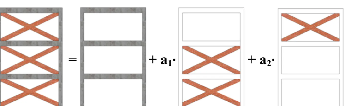
0 1 1 , K K K_r   0 2 2 , K K K_r   ∙ (2.1) ∙ ∙ 0 , K K K_r_N  _N 

therefore, the total stiffness matrix can be reconstructed in the following way: N r N r r T K a K a K a K K  ₀ ₁ _,₁ ₂ _,₂    _, (2.2) in which a₁,a₂,,a_Nare the unknown parameters.

This procedure is illustrated graphically in an example of two bays three storey infilled frame, with two parameters, in Figure 2.1.

2.2.2 Eigenvalues/Eigenvectors problem

In order to define the new target function, the global eigenvalues/eigenvectors problem has to be analyzed. The problem can be set in the following way:













                                             _ _ _ _ 



   n n n N s rs s n i i i N s s rs i N s rs s a p a p a p       φ M K K φ M K K φ M K K 2 1 , 0 2 1 , 0 1 1 2 1 1 , 0 1   (2.3)

in which K₀,K_r_,_s are matrices previously defined, _i is the i-th experimentally identified frequency,



_i is the corresponding experimentally identified mode shape, _i is the vector of residue deriving from the equations of i-th frequency and mode shape. If the exact value of