Nonparametric inference for functional-on-scalar linear models applied to knee kinematic hop data after injury of the anterior cruciate ligament

(1)

DOI: 10.1111/sjos.12333

Scandinavian Journal of Statistics O R I G I N A L A R T I C L E

Nonparametric inference for

functional-on-scalar linear models applied to

knee kinematic hop data after injury of the

anterior cruciate ligament

Konrad Abramowicz

1

_{Charlotte K. Häger}

2

_{Alessia Pini}

3,4

Lina Schelin

2,3

_{Sara Sjöstedt de Luna}

1

_{Simone Vantini}

5

1_{Department of Mathematics and}

Mathematical Statistics, Umeå University, Umeå, Sweden

2_{Department of Community Medicine}

and Rehabilitation, Umeå University, Umeå, Sweden

3_{Department of Statistics, Umeå School}

of Business, Economics and Statistics, Umeå University, Umeå, Sweden

4_{Department of Statistical Sciences,}

Università Cattolica del Sacro Cuore, Milan, Italy

5_{MOX - Modelling and Scientific}

Computing Laboratory, Department of Mathematics, Politecnico di Milano, Milan, Italy

Correspondence

Alessia Pini, Department of Statistical Sciences, Università Cattolica del Sacro Cuore, 20123 Milan, Italy. Email: alessia.pini@unicatt.it; alessia.pini@polimi.it

Funding information

Swedish Scientific Research Council, Grant/Award Number:

K2014-99X-21876-04-4, 340-2013-5203, and 2016-02763; Västerbotten County Council, Grant/Award Number: ALF VLL548501 and VLL-358901 Project No. 7002795

Abstract

Motivated by the analysis of the dependence of knee move-ment patterns during functional tasks on subject-specific covariates, we introduce a distribution-free procedure for testing a functional-on-scalar linear model with fixed effects. The procedure does not only test the global hypoth-esis on the entire domain but also selects the intervals where statistically significant effects are detected. We prove that the proposed tests are provided with an asymptotic control of the intervalwise error rate, that is, the probability of falsely rejecting any interval of true null hypotheses. The procedure is applied to one-leg hop data from a study on anterior cruciate ligament injury. We compare knee kine-matics of three groups of individuals (two injured groups with different treatments and one group of healthy con-trols), taking individual-specific covariates into account.

K E Y WO R D S

analysis of covariance, functional data, human movement, intervalwise testing, permutation test

. . . .

This is an open access article under the terms of the Creative Commons Attribution License, which permits use, distribution and reproduction in any medium, provided the original work is properly cited.

(2)

1 I N T RO D U CT I O N

Functional data analysis is a dynamically developing research area within the field of statis-tics. In recent literature, linear models for functional data have been widely studied (see, e.g., Abramovich & Angelini, 2006; Abramowicz et al., 2014; Cardot, Prchal, & Sarda, 2007; Fan & Zhang, 2000; Fogarty & Small, 2014; Gertheiss, Goldsmith, Crainiceanu, & Greven, 2013; Reiss, Huang, & Mennes, 2010).

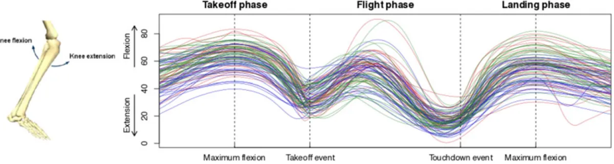
Motivated by the analysis of the dependence of knee movement patterns during functional tasks on subject-specific covariates, we consider in the present paper a functional-on-scalar lin-ear model. Specifically, we model a functional response with a set of covariates multiplied by functional parameters. Such models find their applications in a wide range of research fields where modern techniques enable the collection of high-resolution time-continuous data. In this context, many of the empirically relevant questions address the effect of covariates on a func-tional response. They may also desire the identification of significant domain subsets, that is, time intervals characterized by significant effects of a specific covariate. The incitement for this work comes from a follow-up study after anterior cruciate ligament (ACL) injury. ACL injuries are common worldwide, especially in sports, and are typically treated conservatively either with physiotherapy or with reconstructive surgery in combination with physiotherapy. We analyze the knee-joint kinematics data of a sagittal plane, that is, knee flexion/extension, during a one-leg hop for distance for n = 95 individuals (see Figure 1). We compare individuals from the surgery and physiotherapy groups with healthy-knee controls matched with age and sex.

Previous studies indicated differences in the movement patterns between these groups (Hébert-Losier et al., 2015; Tengman, Grip, Stensdotter, & Häger, 2015). Tengman et al. (2015) had a limitation because it is only considering selected landmarks (events) of the curves. The previ-ous analysis included group effects and covariates but did not take into account the information coming from the functional nature of the data. In the work of Tengman et al. (2015), the complete functional data were considered but without taking covariates into account. Both these studies indicate less knee flexion among the individuals treated with physiotherapy compared with the control group. Here, we overcome both the aforementioned limitations by introducing a statistical tool that both exploits the functional nature of the data and takes into account possible covariate effects. In this paper, we investigate if these differences are only due to group effects or if they can be explained by means of additional individual-specific covariates. Furthermore, the introduced methodology enables the detection of the intervals where the covariates have significant effects

FIGURE 1 Knee flexion and extension in the (left) sagittal plane and (right) flexion/extension angle curves of the (blue) physiotherapy, (red) reconstructive surgery, and (green) control groups. Higher values indicate greater knee flexion [Colour figure can be viewed at wileyonlinelibrary.com]

(3)

(domain selection). Such information provides additional insight into the importance of different time segments of the movement. For instance, the active preparation phase with, for example, knee bending, prior to the actual takeoff of the jump determines much of the performance, but there is no obvious single event that would necessarily be the most representative for the com-parison of movement control for individuals or groups. Likewise, the control of the knee in the landing phase is essential for maintaining balance during the task, but it is not known to a full extent how this is controlled or even how to best assess it. The present method enables compar-isons of the whole movement pattern tailored also to individuals and may, in addition, help in identifying critical intervals within the larger phases of the movement execution.

Parameter estimation of the functional model is handled by least squares estimation, as suggested, for instance, by Ramsay and Silverman (2005). However, forming valid tests of var-ious hypotheses about the functional regression parameters, with the control of the error rate, is not straightforward. One solution adopted in the literature is to develop global tests for the parameters of the model (Abramovich & Angelini, 2006; Antoniadis & Sapatinas, 2007; Cardot et al., 2007; Cuesta-Albertos & Febrero-Bande, 2010; Cuevas, Febrero, & Fraiman, 2004; Kayano, Matsui, Yamaguchi, Imoto, & Miyano, 2015; Schott, 2007; Staicu, Li, Crainiceanu, & Ruppert, 2014; Zhang & Liang, 2014). Such tests investigate if a covariate has a significant effect on the response but does not provide any domain selection. Another approach, proposed by Fan and Zhang (2000), Reiss et al. (2010), and Ramsay and Silverman (2005), is to provide pointwise confi-dence bands for the functional parameters. The results indicate which parts of the domain that the covariates have an effect, with only a pointwise control of the type I error rate. As clearly discussed in the work of Ramsay and Silverman (2005, pp. 243–244), pointwise limits are not equivalent to confidence regions for the entire estimated curves.

Assuming that data are expressed through a functional basis, inference can be based directly on the expansion coefficients, as proposed, for instance, by Spitzner, Marron, and Essick (2003) and Pini and Vantini (2016). In the latter work, single-component tests are performed and their p values adjusted with multiple testing methods. In this way, results are compensated for the many dependent tests performed on the same data set. A drawback with this type of procedures is that they rely on the basis expansion. The test conclusions thus depend on the type of functional basis selected to initialize the methods.

Vsevolozhskaya et al. (2013) and Vsevolozhskaya, Greenwood, and Holodov (2014) proposed an inferential procedure in the functional analysis of variance (ANOVA) framework based on partitioning the domain into preselected subintervals. The procedure, relying on permutation tests, results in a selection of subintervals where significant differences are observed between groups. However, the test conclusions depend on the initially chosen partition and do not take into account covariates.

In the framework of testing differences between two populations, Pini and Vantini (2016) proposed the intervalwise testing (IWT) procedure that tests functional hypotheses and selects intervals of the domain where the null hypothesis is rejected. The procedure relies on the definition of an adjusted p value function provided with a control of the intervalwise error rate (IWER), that is, control of the probability of wrongly rejecting any interval of the domain.

Assuming continuity of the functional data, it is possible to discretize the domain on a fine grid and perform inference separately for each point of the grid. In multivariate data analysis, sev-eral techniques have been proposed in the statistical literature to adjust such univariate p values controlling the familywise error rate (FWER; e.g., Holm, 1979; Holmes, Blair, Watson, & Ford, 1996; Marcus, Eric, & Gabriel, 1976). However, the well-known Bonferroni or Bonferroni–Holm adjustments are not suitable for the case of discretized functional data because their power tends

(4)

to zero as the number of components (points of the grid) increases. Another popular alternative, the closed testing procedure (Marcus et al., 1976), becomes computationally impractical as the number of points of the grid increases. One of the operational methods that can be straightfor-wardly applied to discrete pointwise evaluations of functional data in the t-test framework was proposed by Holmes et al. (1996). It was extended to the case of vector-on-scalar linear models with high-dimensional responses by Winkler, Ridgway, Webster, Smith, and Nichols (2014) and

is based on the maximum of the F-test statistics for global tests, therefore called an Fmax

proce-dure. This procedure can be used for domain selection even if no information on a partition of the domain is available, and it does not require a basis expansion.

In our work, we extend the IWT framework proposed by Pini and Vantini (2017) to the functional-on-scalar linear model to test various hypotheses on the functional coefficients and prove that the proposed tests are exact or asymptotically exact. We utilize tests based on per-mutations, and hence, the procedure does not require normality of the residual functions and knowledge about the covariance structure of the data. We study the performance of our proce-dure on the kinematics data and in a small simulation study. The simulation study investigates the performance of the the IWT procedure. In addition, it includes a comparison of IWT with

the Fmaxprocedure originating from the multivariate setting, to shed light on the behavior of the

latter procedure adapted to the functional data framework.

The paper is outlined as follows. In Section 2, we describe the functional-on-scalar linear model, discussing the methodology proposed for functional parameter estimation and inference. Section 3 reports the theoretical properties of the proposed methodology. The proofs of theorems in Section 3 are reported Section A of the Appendix. In Section 4, we provide the implementation details of the proposed procedure. In Section 5, we report the results of the analysis of the kine-matics data, whereas in Section 6, we present the results of the simulation study. Finally, Section B of the Appendix reports some algorithmic details on the permutation scheme used to perform inference, and Sections C and D of the Appendix report supplementary results on the kinematics data. All computations and plots have been created using R (R Core Team, 2017).

2 M ET H O D O LO GY

2.1 The functional-on-scalar linear model

Suppose we have observed a sample of n-continuous squared integrable random functions

y_i(t), t ∈ [a, b], i = 1, … , n, that is, y_i(·) ∈ C0[a, b] ∀i. We want to study the following

functional-on-scalar linear model: 𝑦i(t) =𝛽0(t) +

L ∑

l=1

𝛽l(t)xli+𝜀i(t), ∀i = 1, … , n, t ∈ [a, b], (1)

where x1i, … , xLi ∈ R are known scalar covariates and𝛽l(t), l = 0, … , L, are the unknown

fixed functional regression parameters. The errors𝜀i(t), t ∈ [a, b] are independent and identically

distributed (with respect to units) zero-mean random functions (not necessarily Gaussian) with finite total variance, that is,

∫ b a

E[𝜀i(t)]2dt< ∞, ∀i = 1, … , n. (2)

(5)

2.2 Model estimation

The ordinary least squares (OLS) estimators of the functional parameters𝛽_l(t), l = 0, … , L, can be

found by minimizing the sum over units of the squared L2distances between the functional data

y_i(t)and the quantity𝛽0(t) +

∑L

l=1𝛽l(t)xliwith respect to𝛽l(t), l = 0, … , L, (Ramsay & Silverman,

2005), hence minimizing n ∑ i=1∫ b a ( 𝑦i(t) −𝛽0(t) − L ∑ l=1 𝛽l(t)xli )2 dt. (3)

From the interchangeability of summation and integration in (3), it follows that minimization can be done separately for each point of the domain, independently of the covariance structure

of the errors𝜀i(t). The OLS estimate ̂𝜷n(t) = ( ̂𝛽0(t), … , ̂𝛽L(t))′, t ∈ [a, b], minimizing (3), can thus

be calculated pointwise for each given t as follows:

̂𝜷n(t) = argmin 𝛽0(t), … ,𝛽L(t) n ∑ i=1 ( 𝑦i(t) −𝛽0(t) − L ∑ l=1 𝛽l(t)xli )2 . (4)

For each t, ̂𝜷_n(t)is thus the OLS estimator of the corresponding scalar-on-scalar linear model at

point t.

Asymptotic properties for the OLS estimates at each point t can be immediately derived from

classical results for scalar-on-scalar linear models. In detail, let Xn be the design matrix Xn ∈

R(n×(L+1))_([X

n]i,1 = 1, ∀i = 1, … , n; [Xn]i,j =xj−1,i, i = 1, … , n, j = 2, … , L + 1). Consider the

following standard conditions.

C1 The matrix X′

nXnis nonsingular, and the inverse V = (Xn′Xn)−1is such that the elements

[V ]ij→ 0 as n → ∞, for all i, j = 1, … , L + 1.

C2 For each t ∈ [a, b], the regression errors 𝜀i(t)satisfy the following:

E[𝜀i(t)2 ]

< ∞.

Under conditions C1 and C2, we have that, for each t ∈ [a, b], the OLS estimate

̂𝜷n(t) = (Xn′Xn)−1Xn′(𝑦1(t), … , 𝑦n(t))′ (5)

is a strongly consistent estimate of𝜷(t) = (𝛽₀(t), … , 𝛽_L(t))′(Lai, Robbins, & Wei, 1979). Condition

C1is a sufficient condition for finding an explicit expression of the OLS estimates and guarantees

convergence in probability. Condition C2 ensures almost sure convergence.

2.3 Model inference

One of the main challenges with inference for functional linear models (1) is to perform valid tests of various hypotheses on the functional regression parameters and to select significant intervals of the domain. For instance, we are interested in the overall model test that none of the covariates have the functional version of the classical F-test hypotheses as follows:

{

H0,F∶𝛽l(t) =0, ∀l ∈1, … , L, ∀t ∈ [a, b]

H1,F∶𝛽l(t)≠ 0, for some l ∈ {1, … , L} and some t ∈ [a, b],

(6)

together with tests on single functional parameters, that is, the functional version of the classical

t-test hypotheses, as follows:

{

H0,l∶𝛽l(t) =0, ∀t ∈ [a, b]

H1,l∶𝛽l(t)≠ 0, for some t ∈ [a, b],

(7)

where l ∈ {0, … , L}.

It may also be of interest to test hypotheses on one or more linear combinations of the func-tional parameters of the regression, specified by a combination matrix C. In detail, let C ∈

R(q×(L+1)) _{be any real-valued full rank matrix, where q denotes the number of hypotheses on}

the functional regression parameters to be jointly tested, with 1 ≤ q ≤ L + 1. Moreover, let

c0(t) = (c01(t), … , c0q(t)) ′

be a vector of fixed functions in C0[a, b]. The general testing problem

can typically then be formulated as follows: {

H0,C∶C𝜷(t) = c0(t), ∀t ∈ [a, b]

H1,C∶C𝜷(t) ≠ c0(t), for some t ∈ [a, b],

(8)

where the jth element of vector C𝜷(t) is a function obtained by means of a linear combination

of the functional regression parameters𝛽l(t) with weights [C]jl: [C𝜷(t)]𝑗 = ∑Ll=0[C]𝑗l𝛽l(t), j =

1, … , q. There are two important special cases of the general functional linear hypotheses (8) as follows.

1. Let q = L, C = CF = (0|IL) ∈ RL×(L+1), and c𝟎(t) = 0 ∈ RL, where IL is the L × L identity

matrix. Then, the hypotheses of (8) correspond to the hypotheses in (6).

2. For a fixed l, let q = 1, C = Cl ∈R1×(L+1)with [Cl]r =1 if r = l and 0 otherwise, and c(t) = 0.

Then, the hypotheses in (8) correspond to the hypotheses in (7).

For test (8), in case of rejection of the null hypothesis H0,C, we want to select the intervals

on [a, b] where significant differences are detected. In theory, this problem can be addressed by

performing an infinite family of tests along the domain [a, b], of the form as follows:

{ Ht

0,C∶C𝜷(t) = c0(t)

H₁t_,C∶C𝜷(t) ≠ c0(t).

(9)

Based on classical results for scalar-on-scalar linear models, it is rather straightforward to test hypotheses (9) for each t. The challenge is to control the FWER arising from the uncountable infinite number of (dependent) hypotheses tests. In this paper, we extend the domain selection IWT procedure by Pini and Vantini (2017) to functional-on-scalar linear models to control the probability of wrongly rejecting each interval characterized by only true hypotheses, that is, the

control of the IWER. The result of the procedure is an adjusted p value function ̃𝑝C(t)for testing

(9) provided with a control of the IWER. The adjusted p value function can be thresholded at level 𝛼 to select the portions of the domain imputable for the rejection of the null hypothesis H0,C. This

type of control guarantees that, for every interval of the domain where H0,Cis true (i.e., where

C𝜷(t) = c0(t)), the probability that H0,Cis rejected at least at one point of the interval is less or

equal to𝛼. The domain selection procedure that we propose is based on three steps presented in

(7)

2.3.1 First step: IWT

Given any closed interval ⊆ [a, b], we want to test the following:

{

H₀_,C∶C𝜷(t) = c0(t), ∀t ∈ 

H₁_,C∶C𝜷(t) ≠ c0(t), for some t ∈ .

(10) To perform tests of linear hypotheses (10), we propose to use the statistics as follows:

T_C_{= ∫}  TC(t)dt, (11) where TC(t) = ( C ̂𝜷(t) − c0(t) )′( C ̂𝜷(t) − c0(t) ) , (12)

and ̂𝜷(t) is the OLS estimate (5). In particular, for the overall model hypotheses on 

{

H₀_,F∶𝛽l(t) =0, ∀l ∈ 1, … , L, ∀t ∈ 

H₁_,F∶𝛽l(t)≠ 0, for some l ∈ {1, … , L} and t ∈ ,

(13) we use the following statistics:

T_F _{= ∫}  L ∑ l=1 ( ̂𝛽ln(t)) 2_dt_. ₍₁₄₎

For the hypotheses of the lth functional regression parameter on

{

H₀_,l ∶𝛽l(t) =0, ∀t ∈ 

H₁_,l ∶𝛽l(t)≠ 0, for some t ∈ ,

(15) we use the test statistics as follows:

T_l _{= ∫}

( ̂𝛽ln(t)

)2

dt. (16)

Note that we have chosen T_Fand T_l to be the special cases of T_C.

2.3.2 Second step: Adjusted p value functions

Let𝑝_Cdenote the p value of test (10) obtained using functional permutation tests based on the

Freedman and Lane permutation scheme (Freedman & Lane, 1983), as defined by Pesarin and Salmaso (2010). It is based on the permutation of the estimated residuals under the reduced model, that is, the linear model constrained to the null hypothesis of the test. The p value of the permutation test is then obtained by calculating the proportion of permutations leading to a larger value of the test statistics than the test statistics on the observed data. This scheme is the most commonly used scheme for linear models and presents many advantages compared with other permutation techniques (Anderson & Legendre, 1999; Anderson & Robinson, 2001; Davison & Hinkley, 1997; Winkler et al., 2014; Zeng, Pan, MaWhinney, Barón, & Zerbe, 2011). In particu-lar, it can be shown empirically that its power is typically higher than the power of tests based on other permutation schemes (Anderson & Legendre, 1999; Winkler et al., 2014). For more details, see Appendix B.

(8)

In order to identify significant subdomains, we make use of adjusted p value functions. The

adjusted p value function ̃𝑝C(t)at point t for testing general linear hypotheses with contrast C is

defined as the supremum p value of all intervalwise tests on intervals containing t, as follows: ̃𝑝C(t) = sup

∶t∈𝑝 

C, t ∈ [a, b]. (17)

Analogously, denoting by 𝑝_F, and𝑝_l the p values from testing Equations 13 and 15,

respec-tively, the adjusted p value functions for testing hypotheses on the overall model and on the lth functional parameter are defined as

̃𝑝F(t) = sup ∶t∈𝑝  F; ̃𝑝l(t) = sup ∶t∈𝑝  l, t ∈ [a, b], (18) respectively.

Due to the nature of permutation tests used here, the adjusted p value functions are quantized continuous functions with the step size decreasing as the sample size n tends to infinity. The continuity of the limiting function is guaranteed by the continuity of the pointwise test statistics

and of the observed functions y_i(t).

2.3.3 Third step: Domain selection

The intervals of the domain presenting a rejection of any of the null hypotheses are obtained by

thresholding the corresponding adjusted p value functions at level𝛼. For example, we select the

intervals presenting at least one significant effect by thresholding ̃𝑝F(t)and intervals presenting a

significant effect of the lth covariate by thresholding ̃𝑝l(t).

The introduced domain selection procedure is provided with a (asymptotic) control of the IWER. This type of control implies that the probability of detecting false positive intervals is

(asymptotically) controlled at level 𝛼. The supporting theoretical results are presented in the

following section.

3 T H EO R ET I C A L R E S U LT S

Here, we present the theoretical properties of the permutation-based inference on functional-on-scalar linear models performed along the line depicted in Section 2. All proofs are reported in Appendix A.

First, we prove that the domain selection IWT procedure for testing general linear hypothesis is provided with an asymptotic control of the IWER. Pini and Vantini (2016) proved that, if all intervalwise tests used to build IWT are exact, the IWT is provided with a control of the IWER. This result can be applied directly in the case of the overall functional model test on the regression model but has to be extended in the more general case of tests on linear hypotheses (including tests on single functional parameters) because, in the latter case, the exactness of all tests is only asymptotical.

Theorem 1. Under assumptions C1 and C2, the domain selection procedure for testing general

functional linear hypotheses is provided with an asymptotic control of the IWER. Formally, the adjusted p value function ̃𝑝C(t) is such that, ∀𝛼 ∈ (0, 1],

∀ ⊆ [a, b] ∶ H

0,C is true ⇒ lim sup

n→∞ P

[∀t ∈, ̃𝑝C(t)≤ 𝛼] ≤ 𝛼.

Because tests on single functional parameters are specific cases of linear hypotheses, we obtain directly the following corollary.

(9)

Corollary 1. Under assumptions C1 and C2, the domain selection procedure for testing

hypotheses for single functional regression parameter is provided with an asymptotic control of the IWER.

Furthermore, the following proposition provides exact results for IWT-based overall func-tional model tests.

Proposition 1. The domain selection procedure for testing the overall functional model

hypotheses is provided with a control of the IWER. Formally, the adjusted p value function ̃𝑝F(t)

is such that, ∀𝛼 ∈ (0, 1],

∀ ⊆ [a, b] ∶ H

0,F is true ⇒P[∀t ∈, ̃𝑝F(t)≤ 𝛼] ≤ 𝛼.

Next, we focus on the property of consistency of the proposed tests. The following theorem

states that the probability of detecting every interval, such that ∀ t ∈  Ht

0,Cis false, converges

to 1 as the sample size increases. This property implies that the probability of truly detecting any point where the null hypothesis is false converges to 1.

Theorem 2. The domain selection procedure for testing general functional linear hypotheses is

consistent. Formally, ∀𝛼 ∈ (0, 1] the adjusted p-value ̃𝑝C(t) is as follows:

∀ ⊆ [a, b] such that Ht

0,C is false ∀t ∈ ⇒ limn→∞P[∀t ∈, ̃𝑝C(t)≤ 𝛼] = 1.

As a consequence, we also obtain consistency results for the IWT-based tests of the overall functional model and on single functional parameters.

Corollary 2. The domain selection procedure for the overall functional model hypotheses is

consistent.

Corollary 3. The domain selection procedure for single functional parameter hypotheses is

consistent.

4 D ETA I L S O N T H E I M P L E M E N TAT I O N

In practice, evaluations of the adjusted p value functions, even at one fixed point t ∈ [a, b],

are practically infeasible because it involves taking supremum over uncountably many subin-tervals covering point t. We therefore propose a numerical procedure resulting in pointwise constant approximation of the p value functions and the significance regions chosen accordingly. The approximation error of the procedure is dependent on two parameters. The first parameter,

K ∈ N, defines the size of the initial partition of interval [a, b]. The second parameter, B ∈ N,

determines the number of random permutations used in the conditional Monte Carlo algorithm (Pesarin & Salmaso, 2010) to approximate the intervalwise permutation tests p values.

The following steps describe the procedure for linear hypotheses of the functional parameters with combination matrix C.

Step 1 Partition the domain [a, b] into K equally sized atomic subintervals of length Δt = (b −

a)∕K, that is,

i= [a + (i −1)Δt, a + iΔt] i =1, … , K.

Let be the family (of size K(K + 1)∕2) of all possible intervals constructed from the K

(10)

Step 2 For i = 1, … , K, approximate the value of the integrated test statistics Ti

C by

̂ 𝑇i

𝐶 =TC(a + (i −1)Δt) Δt.

This is equivalent to approximating the pointwise test statistics TC(t)in atomic

subin-tervals Piwith a constant equal to TC(a + (i −1)Δt), that is, the value of the statistics in

the left endpoint of the interval Pi.

Step 3 For all intervals ∈ , approximate the value of the integrated test statistics by

̂_T C = ∑ i⊂ ̂_Ti C .

The approximations of the integrated test statistics correspond to a rectangle quadrature

with step Δt applied to the pointwise test statistics TC(·).

Step 4 Estimate the p values ̂𝑝_C of the tests on each ∈  using the Freedman and Lane permutation scheme (see Appendix B) with B randomly chosen permutations.

Step 5 The adjusted p value function at point t is estimated by the maximum of the

correspond-ing p values of all intervals in  containing t, that is,

̂_̃𝑝_C(t) =max{ ̂̃𝑝_C ∶ ∈  such that t ∈ 

} .

Furthermore, by construction, ̂̃𝑝C(t)is constant at each atomic subinterval, and

there-fore, the estimate of ̃𝑝C(t)for all t ∈ [a, b] is obtained by evaluating the above maximum

Ktimes (one time per1, … , K).

Step 6 Select the significant domain subset by thresholding the obtained approximated

adjusted p value function.

Observe that, as K tends to infinity, the error arising due to the discretization of the domain

becomes negligible. This is guaranteed by the integrability of the pointwise test statistics TC(t)and

resulting continuity of the integrated test statistics with respect to the integration limits. Further-more, as the number of simulated permutations B increases, the Monte Carlo error tends to zero. It is worth to notice that in Step 4, we use the same B permutations for each subinterval, which decreases the computational complexity of the algorithm.

5 A NA LY S I S O F K N E E K I N E M AT I C S

We will now report the results of the analysis of the knee kinematics data briefly presented in the introduction. To investigate potential long-term differences in movement patterns following ACL injury, individuals treated with either reconstructive surgery in combination with physiotherapy

(ACLR) or physiotherapy alone (ACLPT) were tested in a motion laboratory. The resulting

func-tional data consist of the joint angle motion in different movement planes during a one-leg hop, sampled at 240 Hz.

The functional data set that we analyze here corresponds to the knee movement in the sagit-tal plane, that is, knee flexion/extension (see Figure 1) during a one-leg hop for distance. Our

primary focus is to compare (ACLR) and (ACLPT) individuals with healthy-knee controls (CTRL)

matched with age and sex, taking individual-specific covariates into account. The three groups are only matched on group level (Hébert-Losier et al., 2015), and hence, age and sex are included as possible covariates together with available data about jump length and body mass index (BMI). The knee movement in the sagittal plane for the hop of maximal length (out of three attempts)

(11)

on the injured leg for the two ACL groups was compared with the nondominant leg for controls. In the case of group differences, it is of clinical interest to find out which time intervals of the jump these differences occur. Functional data were recorded at 240 Hz using a calibrated 8-camera 3D motion analysis system. Kinematic parameters were calculated using rigid-body analysis and

Euler angles. Knee-joint angles (◦) were computed using an x-y-z Cardan sequence equivalent to

the knee-joint coordinate system. The knee-joint kinematic curves in the sagittal plane of motion were extracted and smoothed through a functional B-spline basis with 150 equally spaced knots. In order to take into account the different time lengths, data were aligned by means of four land-marks: the event of maximal knee flexion before takeoff, the takeoff event (the instant at which the foot leaves the ground), the touchdown event (the time instant at which the foot touches the ground), and the event of maximal knee flexion after landing. The aligned data and the landmarks are displayed in the right panel of Figure 1. For more details on data collection and preprocessing, we refer to the work of Hébert-Losier et al. (2015). The hop consists of three phases: time preced-ing the takeoff event (takeoff phase), time between the takeoff event and the landpreced-ing event (flight phase), and time succeeding the landing event (landing phase).

The initial model we use to describe the knee-joint angle motion in the sagittal plane, yi(t), is

the following:

𝑦i(t) =𝛽0(t) +𝛽Jump(t)xJump,i+𝛽BMI(t)xBMI,i+𝛽Age(t)xAge,i

+𝛽Sex(t)xSex,i+𝛽CTRL(t)xCTRL,i+𝛽R(t)xR,i+𝜀i(t), i = 1, … , 95,

where the covariates xJump,i, xBMI,i, and xAge,iindicate the jump length, BMI, and age, respectively,

of individual i. Furthermore, xSex,i, xCTRL,i, and xR,iare indicator functions attaining the value of 1

if individual i is a man in the control group and in the reconstructive surgery group, respectively, and otherwise 0.

As in classical multiple regression, we start with the initial model using all available covariates and then use backward elimination to reduce it to a final model that includes only the significant covariates. We start by performing a global overall significance test that simultaneously tests if at least one of the coefficients is significant somewhere on the domain; compare (6). Separate global tests are then performed for each coefficient as in (7). Table 1 presents the p values obtained by performing permutation tests with B = 1000 and test statistics Equations 14 and 16, where the

interval corresponds to the whole domain. Starting from these results, we apply the backward

elimination procedure and stepwise remove the covariates with the largest p value (one at a time, and re-estimate the reduced model) until only the significant coefficients remain in the model. We use a 5% significance level at all steps of the procedure. The final model includes the continuous covariate Jump and the group indicators. The corresponding p values are presented in Table 2.

After assessing the overall significance of the covariates on the whole domain, we apply the introduced IWT-based procedure to the study in which parts of the domain, the coeffi-cients, are significant. To illuminate all between-group differences, we use suitable combination matrices and introduce an additional hypothesis comparing the performance of the control and

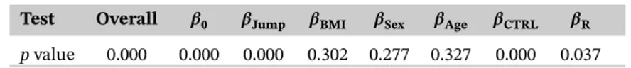
TABLE 1 Global p values of the initial model for the overall test (6) and for each single functional parameter test (7) obtained by performing permutation tests with B = 1,000 based on test statistics in Equations 14 and 16, respectively

Test Overall 𝜷₀ 𝜷_Jump 𝜷_BMI 𝜷_Sex 𝜷_Age 𝜷_CTRL 𝜷_R

(12)

TABLE 2 Global p values of the reduced final model for the overall test (6) and for each single functional parameter test (7) obtained by performing permutation tests with

B =1,000 based on test statistics in Equations 14 and 16, respectively

Test Overall 𝜷₀ 𝜷_Jump 𝛽_CTRL 𝛽_R

pvalue 0.000 0.000 0.000 0.000 0.029

reconstructive surgery groups (see below). The adjusted p value functions are computed according to Section 4 with K = 300 and B = 1000.

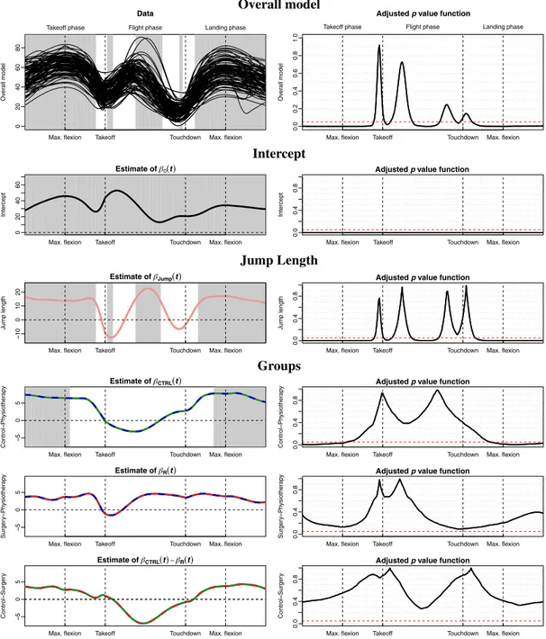
Functional parameter estimates together with estimated adjusted p value functions for the overall functional model and single functional parameter tests are given for the final model in Figure 2. For illustrative purposes, we also present the results of the ITW-based procedure for the full model in Appendix C.

The first row in Figure 2 shows the individual knee-joint angle kinematics curves (left) and, in black solid line, the estimated adjusted p value functions for the overall functional tests (right), indicating the presence of at least one significant effect in the majority of the jump. The gray-shaded parts of the domain (left) correspond to significant effects at the 5% level (i.e., the

points t with associated adjusted p values≤ 0.05, indicated with a dashed red line in the right

panel).

As expected, the jump length has a significant effect throughout all three jump phases, in the

majority of the domain (Figure 2, row 3). The functional parameter estimate ̂𝛽Jumpn(t)is positive

in intervals containing the maximal flexion during both takeoff and landing and negative directly after takeoff and just before touchdown, confirming that the movement is more pronounced for longer jumps. The parts of the domain where the effect is nonsignificant are expected because

𝛽Jump(·)is anticipated to change sign.

The last three rows of Figure 2 present results of group comparisons, testing respectively

H0,CTRL−PT∶𝛽CTRL(t) =0, H1,CTRL−PT∶𝛽CTRL(t)≠ 0,

H0,R−PT∶𝛽R(t) =0, H1,R−PT∶𝛽R(t)≠ 0,

H0,CTRL−R∶𝛽CTRL(t) −𝛽R(t) =0, H1,CTRL−R∶𝛽CTRL(t) −𝛽R(t)≠ 0,

with the parameter estimates to the left and corresponding adjusted p value functions to the right.

The ACLPT group is significantly different with respect to the control group during both

take-off and landing (Figure 2, row 4). The functional parameter estimate ̂𝛽CTRLn(·)associated to the

differences indicates less flexion in the ACLPT group during these two phases compared with

individuals in the control group because there, ̂𝛽CTRLn(t)is positive. These results are in line with

previously reported results (Hébert-Losier et al., 2015; Tengman et al., 2015), indicating significant differences between physiotherapy-treated individuals and controls. We do not detect any signifi-cant differences between the reconstructive surgery group and the controls (Figure 2, row 6). The

overall test of𝛽R(·)indicates that the reconstructive surgery group is significantly different from

the ACLPTgroup (Table 2). However, there is no sufficient evidence to identify which parts of the

domain the significant differences between the two groups occur (the corresponding adjusted p value function never goes below the 5% level); compare Figure 2, row 5.

We observe significant group differences between 0% and 56% of the takeoff phase and between 36% and 100% of the landing phase. We thus validate the clinical hypotheses that the preparation of the jump in the takeoff phase and the stabilization in the landing phase are of particular interest in relation to movement control after injury. Our analysis confirms that the

(13)

0 2 04 06 08 0 Data Ov er all model

Takeoff phase Flight phase Landing phase

Max. flexion Takeoff Touchdown Max. flexion

02 0 4 0 6 0 Estimate of 0t Intercept

10 0 1 0 2 0 Estimate of Jumpt J ump length

50 5 Estimate of Rt Surger y Ph ysiother ap y

50 5 Estimate of CTRLt Control Ph ysiother a p y

50 5 Estimate of CTRLt Rt Control Surger y

0.0 0.2 0.4 0.6 0.8 1.0

Adjusted p value function

Ov

er

all model

Takeoff phase Flight phase Landing phase

0.0

0.4

0.8

Intercept

0.0

0

.4

0.8

J

ump length

0.0

0

.4

0.8

Surger y Ph ysiother a p y

0.0

0

.4

0.8

Control Ph ysiother a p y

0.0

0

.4

0.8

Control

Surger

y

Intercept

Jump Length

Groups Overall model

FIGURE 2 (Left) functional parameter estimates and (right) estimated adjusted p value functions for the final (reduced) functional-on-scalar model. Top panel: (left) knee-joint angle kinematics data (functional response variable) for the 95 individuals and (right) estimated adjusted p value function for the overall functional model tests. Bottom panels: (left) functional parameter estimates and (right) corresponding estimated adjusted p value functions for the intercept, jump length, and group effects, respectively. (Left) Gray-shaded parts correspond to significant effects at the 5% level, that is, the points t with associated adjusted p values less or equal to 0.05. (Right) Black solid lines correspond to intervalwise-testing-adjusted p value; (right) red dashed horizontal line corresponds to 5% threshold [Colour figure can be viewed at wileyonlinelibrary.com]

(14)

events of maximal flexion, analyzed for example in the work of Tengman et al. (2015), provides some insight into how the groups may differ. However, basing only on analyses on comparisons of movement data taken at one particular point in time provides limited information, and with the present procedure, we are able to detect significant differences in large parts of the takeoff and landing phases.

As a complement to the analysis of the kinematics data within the IWT framework, in

Appendix D, we report the results with the Fmax procedure applied (see Section 6 for details

about the implementation of Fmax). The Fmaxprocedure provides very similar results to the ones

obtained with our IWT-based procedure, corroborating the results discussed in this section.

6 S I M U L AT I O N ST U DY

In this section, we report the results of a simulation study carried out to investigate the behavior of the IWT procedure and also to make a numerical comparison between the IWT procedure and

the Fmaxprocedure (Holmes et al., 1996; Winkler et al., 2014). Both are nonparametric methods

for performing inference on linear models, and they can be used to perform domain selection.

However, it is important to note that, methodologically, the two procedures differ because the Fmax

procedure is developed for vector-on-scalar linear models, that is, models where the response is a vector of finite dimension and the covariates are scalar.

6.1 F

max

procedure

We start by providing a brief description of the Fmaxprocedure. When applied to vector-on-scalar

linear models in a multivariate setting, the procedure of computing the adjusted p value function can be summarized in the following steps.

Step 1 The overall F-test statistics is computed for every component of the response vector. Step 2 Freedman and Lane permutations (see Appendix B) are applied jointly to all

compo-nents of the response vector.

Step 3 For each permutation, the F-test statistics is computed again for each component, and

the maximum of the permuted statistics over all components is computed.

Step 4 For each component, the F-test statistics based on the observed data is compared

with the permutational distribution of its maximum. The adjusted p value associated to each component is the proportion of permutations where the maximum test statistics is higher or equal to the observed test statistics.

Further details on construction, properties, and implementation of the Fmaxprocedure can be

found in the work of Winkler et al. (2014). One of the eminent properties making the comparison

of our procedure and Fmaxespecially interesting is the strong control of the FWER.

The procedure extends to functional-on-scalar linear models by applying the test to discrete pointwise evaluations of the functional data. In detail, the functional response is discretized on a grid, and a vector-on-scalar linear model is fitted for the discretized response. The pointwise test statistics is compared with the permutational distribution of the maximum of such statistics over the discretized domain.

6.2 Simulation study setting

We simulate functional data according to the following intercept-free linear model: 𝑦i(t) =𝛽1(t)x1i+𝜀i(t) i =1, … , n, t ∈ [0, 1],

(15)

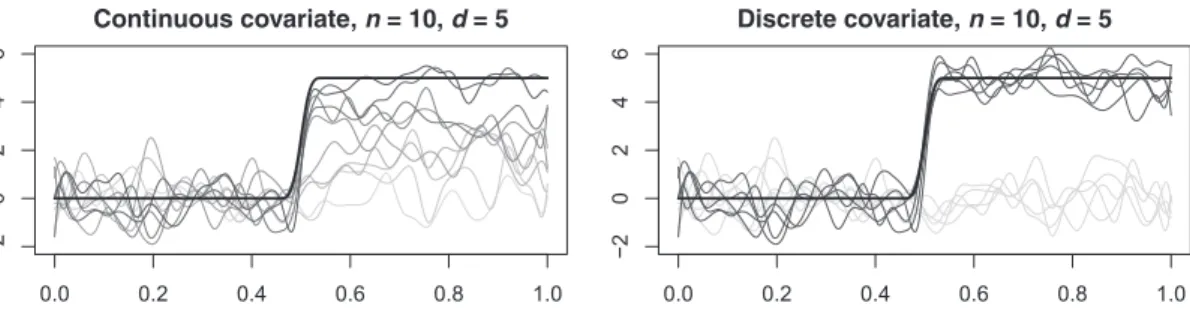
0.0 0.2 0.4 0.6 0.8 1.0 −2 0 2 4 6 Continuous covariate, n = 10, d = 5 0.0 0.2 0.4 0.6 0.8 1.0 −2 0 2 4 6 Discrete covariate, n = 10, d = 5

FIGURE 3 One instance of simulated data with parameters n = 10 and d = 5 and (left) continuous or (right) discrete covariate. Gray levels of the curves are associated to the covariate values (dark: high value; light: low value). The black bold line indicates the functional term d · f(t)

where𝛽₁(t) = d·f(t), d ∈R. The function f(t) is a fixed curve obtained with a cubic B-spline

expan-sion with 40 basis functions. The first 20 coefficients of the expanexpan-sion are set to zero, and the last 20 coefficients are set to one. The resulting function is equal to zero in the first part of the domain

(t ∈ [0, 17∕37]) and to one in the second part of the domain (t ∈ [20∕37, 1]), with a continuous

and differentiable transition between the two parts. With such a definition of f(t), the parameter

dis a magnitude parameter that accentuates the effect of the covariate. The error functions𝜀i(t)

are simulated with the same cubic B-spline basis. The coefficients of the basis expansion are sam-pled independently from a standard normal distribution. We investigate the following two cases for the covariate type.

1. Continuous covariate: x1i= i −1 n −1, i =1, … , n. 2. Discrete covariate: x1i= { 0 i =1, … , n∕2 1 i = n∕2 + 1, … , n.

When evaluating performance, we consider the raster of values d = 0, 0.5, 1, … , 5 together

with three different sample sizes n = 10, 20, 40. We perform the overall tests of H0,Fagainst H1,F

(that, in this case, coincides with the test on𝛽1(t)) with the procedure proposed in this paper and

with the Fmaxprocedure. In the following, we denote by D0the interval of the domain where H0,F

is true and with D1 = D∖D0the interval of the domain where H0,Fis false. For performing the

comparison, the same discretization of functional data based on 50 pointwise evaluations is used for both procedures. An instance of the simulated functional data with n = 10, d = 5, and a continuous or discrete covariate are displayed in Figure 3. The figure displays the functional data in gray with the intensity of the gray color being proportional to the value of the covariate. The term d × f(t) is displayed in both panels with a black bold line.

6.3 Performance measures

Let ̃𝑝(t) denote the adjusted p value function for the F test resulting from the inferential proce-dure. We investigate the behavior of the two procedures in terms of the following quantities (as functions of d).

(16)

1. The estimated FWER, that is, the probability of rejecting H0,Ffor at least one point of D0(where

the null hypothesis is true):

FWER =P[∃t ∈ D0∶ ̃𝑝(t) ≤ 𝛼].

2. The estimated power, that is, the probability of rejecting H0,Ffor at least one point of D1(where

the null hypothesis is false):

Power =P[∃t ∈ D1∶ ̃𝑝(t) ≤ 𝛼].

3. The estimated sensitivity, that is, the average measure of the correctly detected domain over the measure of the domain where the null hypothesis is false:

Sensitivity =E [ |t ∈ D1∶ ̃𝑝(t) ≤ 𝛼| |D1| ] ,

where| · | denotes the Lebesgue measure.

All three quantities are estimated for both procedures with a Monte Carlo simulation based on 1,000 randomly generated data sets.

6.4 Results

The results of the simulations for continuous and discrete covariate types are shown in Figure 4 (first and second row, respectively). First of all, note that, as supported by theory, both procedures control the FWER for all values of d and for all sample sizes. Furthermore, as expected, increasing

dresults in higher power and sensitivity for both procedures. The results in terms of power and

2 4 6 8 10 0.00 0.02 0.04 0.06 0.08 0.10 FWER d Contin uous Co v ariate 2 4 6 8 10 0.0 0.2 0.4 0.6 0.8 1.0 Power d 2 4 6 8 10 0.0 0.2 0.4 0.6 0.8 1.0 Sensitivity d 2 4 6 8 10 0.00 0.02 0.04 0.06 0.08 0.10 FWER d Discrete Co v a riate 2 4 6 8 10 0.0 0.2 0.4 0.6 0.8 1.0 Power d 2 4 6 8 10 0.0 0.2 0.4 0.6 0.8 1.0 Sensitivity d IWT n = 10 n = 20 n = 40 Fmax n=10 n=20 n=40

FIGURE 4 Results of numerical comparison between intervalwise testing (IWT) and Fmaxbased on 1,000

randomly simulated data sets for different values of d and n. Top: continuous covariate; bottom: discrete covariate. Left: estimated familywise error rate (FWER); center: estimated power; right: estimated sensitivity

(17)

sensitivity indicate that (in the case of our data) the IWT procedure appears to be more powerful and more precise with respect to the identification of the interval where the null hypothesis is

violated. This is in line with the fact that the Fmaxis provided with a strong control of the FWER,

whereas the IWT control is only intervalwise. When investigating the figure, we also see that, as the sample size increases, the performance of the two procedures in terms of both power and sensitivity becomes similar.

In addition to presented results, we carried out several additional simulations by changing some of the parameters of the generative model and of the simulation itself. For brevity, we do not report the full results here but provide a short summary. When varying the signal-to-noise ratio or increasing the number of coefficients of the basis expansion, we have found that the IWT

generally appears to be more powerful than Fmax in noisy situations. Conversely, in less noisy

situations, the performance of the two procedures becomes more similar. Furthermore, we have seen that introducing a positive or negative correlation between the coefficients in the error term does not alter the results significantly.

7 D I S C U S S I O N A N D CO N C LU S I O N S

In this work, we have introduced a nonparametric methodology to test the functional parameters of a functional-on-scalar linear model with fixed effects. We provide IWT procedures based on per-mutations to test hypotheses on the functional regression parameters, including domain selection. We show that our proposed IWT-based procedure is asymptotically exact and consistent.

Due to the nonparametric nature of the testing procedures that we propose, the test statistics in Equations 11, 14, and 16 can be replaced by the integrated versions of other feasible pointwise

test statistics, given that they are continuous functions on [a, b]. The continuity of the pointwise

test statistics with respect to t is required to guarantee that the numerical procedure described in Section 4 provides a proper estimate of the adjusted p value functions. If integrable pointwise test statistics are to be used, more sophisticated numerical algorithms that can deal with improper integration need to be used to estimate the adjusted p value functions.

The IWT procedure used in this paper provides control of the IWER. As shown by Pini and Vantini (2016), the control can also be extended to the complementary sets of all intervals. In our

simulation study, we report a numerical comparison with the Fmaxprocedure described in the

work of Winkler et al. (2014), which is provided with a strong control of the FWER. The results

indicate that the IWT and Fmaxprocedures perform similarly in terms of power and sensitivity

with the IWT being superior for smaller sample sizes and more noisy data.

The analysis of the knee kinematics data set showed that the effect of jump length on knee kinematics is significantly different from zero, whereas the effects of BMI, sex, and age are not. In line with previous findings, even after having been discounted for the jump length, the phys-iotherapy group remains significantly different with respect to the control group during takeoff and landing. Our detected significant domain segments confirm the importance of the land-marks analyzed earlier by Tengman et al. (2015) in the problem of identifying group differences, simultaneously indicating statistical differences on wider segments of the time domain.

When performing backward or forward selection of significant covariates in a scalar-on-scalar linear model, the order in which covariates are removed or added to the model can influence the final result. In the case of functional-on-scalar linear models discussed in this paper, the situation could be even more difficult because the adjusted p value for each covariate changes along the domain. Nevertheless, note that backward selection is not the only possibility for select-ing significant covariates. For instance, it is straightforward to define a functional coefficient of

(18)

determination (R2_{) and use it as an index to perform model selection. Also, in this case,}

selec-tion of covariates would not be straightforward because a funcselec-tional R2will also change along the

domain. In the case study presented in the current paper, this was not an issue because the results of the full model (reported in the Appendix) and the ones of the reduced model lead to similar conclusions. In general, a careful study of the results of all steps of backward or forward selection is advised.

Estimation and IWT of functional-on-scalar linear models are of interest in many recent appli-cations. For instance, it could be applied for comparing pulmonary volume over time of different individuals, such as the data analyzed by Fogarty and Small (2014), for comparing hemolysis curves—the percent hemolysis as a function of time—at various treatment levels (Vsevolozhskaya et al., 2014), or for modeling the functional connectivity between brain regions as a function of distance between the regions, as in the work of Reiss et al. (2010). In all the mentioned cases, the methodology proposed in this work would additionally allow the selection of the intervals of the domain (i.e., time or space intervals) presenting significant effects of the covariates.

Even though the technique presented in this paper is meant to deal with functional data with-out requiring any basis expansion, rarely functional data are observed continuously. Usually, they are instead given as discrete observations of some variables. If the approximation described in Section 4 requires another resolution than the one of the raw data, or if the data are irregularly sampled, preprocessing of functional data through a basis expansion is needed. In such a case and in the presence of noisy observations, smoothing has to be performed carefully because both oversmoothing and undersmoothing the data would have as consequence a loss of power of the inferential procedure.

Because IWT aims at selecting the parts of the domain that are responsible for a rejection of a null hypothesis, the registration of functional data will also impact the results. Being a local technique, the IWT essentially compares functional data in terms of amplitude along the domain, implicitly assuming that the functions are without phase variation. In the presence of phase vari-ation, registration is a crucial step of preprocessing because it makes the comparison in terms of amplitude between the different curves possible. An extensive study on the impact of the prepro-cessing (including both smoothing and registration) of functional data on the IWT is beyond the scope of this paper, but it would be of clear interest for future research.

Finally, it would be of interest to extend the domain-selective inference described here to functional-on-functional linear models. In such a framework, the functional regression

coef-ficients 𝛽_l(t) can be replaced by functional linear operators, and the concept of intervalwise

inference has to be extended accordingly. Such a model would allow us to introduce the effects of time-varying covariates on the functional responses and could be of interest in applications where the covariates also change in time. Another possible extension of the methodology proposed in this paper would be to incorporate random effects in the model.

AC K N OW L E D G E M E N T S

Part of this work was funded by the Swedish Scientific Research Council (Häger grant K2014-99X-21876-04-4, Sjöstedt de Luna grant 340-2013-5203, and Schelin grant 2016-02763) and by the Västerbotten County Council (Häger grant ALF VLL548501 and Strategic funding VLL-358901 through Project 7002795).

O RC I D

(19)

R E F E R E N C E S

Abramovich, F., & Angelini, C. (2006). Testing in mixed-effects FANOVA models. Journal of Statistical Planning

and Inference, 136, 4326–4348.

Abramowicz, K., Häger, C., Hébert-Losier, K., Pini, A., Schelin, L., Strandberg, J., & Vantini, S. (2014). An infer-ential framework for domain selection in functional ANOVA. In E. G. Bongiorno, E. Salinelli, A. Goia, & P. Vieu (Eds.), Contributions in infinite-dimensional statistics and related topics (pp. 13–18). Bologna, Italy: Società Editrice Esculapio.

Anderson, M. J., & Legendre, P. (1999). An empirical comparison of permutation methods for tests of partial regression coefficients in a linear model. Journal of Statistical Computation and Simulation, 62, 271–303. Anderson, M. J., & Robinson, J. (2001). Permutation tests for linear models. Australian & New Zealand Journal of

Statistics, 43, 75–88.

Antoniadis, A., & Sapatinas, T. (2007). Estimation and inference in functional mixed-effects models.

Computa-tional Statistics & Data Analysis, 51, 4793–4813.

Cardot, H., Prchal, L., & Sarda, P. (2007). No effect and lack-of-fit permutation tests for functional regression.

Computational Statistics, 22, 371–390.

Cuesta-Albertos, J. A., & Febrero-Bande, M. (2010). A simple multiway ANOVA for functional data. TEST, 19, 537–557.

Cuevas, A., Febrero, M., & Fraiman, R. (2004). An ANOVA test for functional data. Computational Statistics & Data

Analysis, 47, 111–122.

Davison, A. C., & Hinkley, D. V. (1997). Bootstrap methods and their application. Cambridge, UK: Cambridge University Press.

Fan, J., & Zhang, J. T. (2000). Two-step estimation of functional linear models with applications to longitudinal data. Journal of the Royal Statistical Society, Series B: Statistical Methodology, 62, 303–322.

Fogarty, C. B., & Small, D. S. (2014). Equivalence testing for functional data with an application to comparing pulmonary function devices. Annals of Applied Statistics, 8, 2002–2026.

Freedman, D., & Lane, D. (1983). A nonstochastic interpretation of reported significance levels. Journal of Business

& Economic Statistics, 1, 292–298.

Gertheiss, J., Goldsmith, J., Crainiceanu, C., & Greven, S. (2013). Longitudinal scalar-on-functions regression with application to tractography data. Biostatistics, 14, 447–461.

Hébert-Losier, K., Pini, A., Vantini, S., Strandberg, J., Abramowicz, K., Schelin, L., & Häger, C. K. (2015). One-leg hop kinematics 20 years following anterior cruciate ligament ruptures: Data revisited using functional data analysis. Clinical Biomechanics, 30, 1153–1161.

Holm, S. (1979). A simple sequentially rejective multiple test procedure. Scandinavian Journal of Statistics, 6, 65–70.

Holmes, A. P., Blair, R. C., Watson, J. D. G., & Ford, I. (1996). Nonparametric analysis of statistic images from functional mapping experiments. Journal of Cerebral Blood Flow and Metabolism, 16, 7–22.

Kayano, M., Matsui, H., Yamaguchi, R., Imoto, S., & Miyano, S. (2015). Gene set differential analysis of time course expression profiles via sparse estimation in functional logistic model with application to time-dependent biomarker detection. Biostatistics, 17, 235–248.

Lai, T. L., Robbins, H., & Wei, C. Z. (1979). Strong consistency of least squares estimates in multiple regression.

Journal of Multivariate Analysis, 9, 343–361.

Marcus, R., Eric, P., & Gabriel, K. R. (1976). On closed testing procedures with special reference to ordered analysis of variance. Biometrika, 63, 655–660.

Pesarin, F., & Salmaso, L. (2010). Permutation tests for complete data: Theory, applications and software. Chichester, UK: John Wiley & Sons Inc.

Pini, A., & Vantini, S. (2016). The interval testing procedure: A general framework for inference in functional data analysis. Biometrics, 72, 835–845.

Pini, A., & Vantini, S. (2017). Interval-wise testing for functional data. Journal of Nonparametric Statistics, 29, 407–424.

R Core Team (2017). R: A language and environment for statistical computing. Vienna, Austria: R Foundation for Statistical Computing.

(20)

Reiss, P. T., Huang, L., & Mennes, M. (2010). Fast function-on-scalar regression with penalized basis expansions.

International Journal of Biostatistics, 6, 1–28.

Schott, J. R. (2007). Some high-dimensional tests for a one-way MANOVA. Journal of Multivariate Analysis, 98, 1825–1839.

Spitzner, D. J., Marron, J. S., & Essick, G. K. (2003). Mixed-model functional ANOVA for studying human tactile perception. Journal of the American Statistical Association, 98, 263–272.

Staicu, A.-M., Li, Y., Crainiceanu, C. M., & Ruppert, D. (2014). Likelihood ratio tests for dependent data with applications to longitudinal and functional data analysis. Scandinavian Journal of Statistics, 41, 932–949. Tengman, E., Grip, H., Stensdotter, A. K., & Häger, C. K. (2015). Anterior cruciate ligament injury about 20 years

post-treatment: A kinematic analysis of one-leg hop. Scandinavian Journal of Medicine & Science in Sports, 25, 818–827.

Vsevolozhskaya, O. A., Greenwood, M. C., Bellante, G. J., Powell, S. L., Lawrence, R. L., & Repasky, K. S. (2013). Combining functions and the closure principle for performing follow-up tests in functional analysis of variance.

Computational Statistics & Data Analysis, 67, 175–184.

Vsevolozhskaya, O., Greenwood, M., & Holodov, D. (2014). Pairwise comparison of treatment levels in functional analysis of variance with application to erythrocyte hemolysis. Annals of Applied Statistics, 8, 905–925. Winkler, A. M., Ridgway, G. R., Webster, M. A., Smith, S. M., & Nichols, T. E. (2014). Permutation inference for

the general linear model. Neuroimage, 92, 381–397.

Zeng, C., Pan, Z., MaWhinney, S., Barón, A. E., & Zerbe, G. O. (2011). Permutation and F distribution of tests in the multivariate general linear model. The American Statistician, 65, 31–36.

Zhang, J., & Liang, X. (2014). One-way ANOVA for functional data via globalizing the pointwise F-test.

Scandina-vian Journal of Statistics, 41, 51–71.

How to cite this article: Abramowicz K, Häger CK, Pini A, Schelin L, Sjöstedt de Luna

S, Vantini S. Nonparametric inference for functional-on-scalar linear models applied to knee kinematic hop data after injury of the anterior cruciate ligament. Scand J Statist.

2018;1–26.https://doi.org/10.1111/sjos.12333

A P P E N D I XA: P RO O F S

We here provide the proofs of the theorems stated in Section 3. We first report the theoretical properties of the functional intervalwise tests in Equations 10, 13, and 15 based on the Freedman and Lane scheme and on integrated test statistics in Equations 12, 14, and 16. Then, we prove that the IWT-based tests of linear hypotheses on the functional-on-scalar linear model are provided with an asymptotic control of the IWER and that they are consistent. Additionally, we show that the IWT-based F test on the regression model is provided with an exact control of the IWER.

A.1 Intervalwise tests

We start by showing asymptotic exactness of functional tests on linear hypotheses for a given

interval.

Lemma 1. Under assumptions C1 and C2 and for each interval ⊆ [a, b], the functional test of

linear hypotheses on the regression parameters (10) based on statistics T_C(11) is asymptotically exact.

Proof. Let H₀_,Chold, that is, C𝜷(t) = c0(t), ∀t ∈. Under the null hypothesis and for any t ∈ ,

the model can be reduced by solving the linear system C𝜷(t) = c0(t). In particular, because C