Temperature structure in the Perseus cluster core observed with Hitomi

arXiv:1712.06612v1 [astro-ph.HE] 18 Dec 2017

doi: 10.1093/pasj/xxx000

Temperature Structure in the Perseus Cluster

Core Observed with Hitomi

∗

Hitomi Collaboration, Felix A

, Hiroki A

, Fumie

A

, Steven W. A

, Lorella A

, Marc A

,

Hisamitsu A

, Magnus A

, Aya B

, Marshall W.

B

, Roger B

, Laura W. B

, Gregory V.

B

, Esra B

, Edward M. C

, Maria C

,

Meng P. C

, Paolo S. C

, Elisa C

, Jelle

P

,

Cor P.

V

, Jan-Willem

H

, Chris D

, Tadayasu

D

, Ken E

, Megan E. E

, Teruaki E

, Yuichiro

E

, Andrew C. F

, Carlo F

, Adam R. F

,

Ryuichi F

, Yasushi F

, Maki F

, Akihiro

F

, Massimiliano G

, Luigi C. G

, Poshak

G

, Margherita G

, Andrea G

, Liyi G

, Matteo

G

, Yoshito H

, Kouichi H

, Kenji H

,

Ilana M. H

, Isamu H

, Katsuhiro H

,

Takayuki H

, Kiyoshi H

, Junko S. H

, Ann

H

, Akio H

, John P. H

, Yuto I

,

Ryo I

, Hajime I

, Yoshiyuki I

, Manabu I

, Kumi

I

, Yoshitaka I

, Masachika I

, Jelle K

,

Tim K

, Tsuneyoshi K

, Jun K

, Yuichi K

,

Satoru K

, Nobuyuki K

, Richard L. K

, Caroline A.

K

, Takao K

, Shunji K

, Tetsu K

,

Takayoshi K

, Motohide K

, Katsuji K

, Shu

K

, Peter K

, Hans A. K

, Aya K

,

Hideyo K

, Philippe L

, Shiu-Hang L

, Maurice A.

L

, Olivier L

, Michael L

, Knox S.

L

, David L

, Greg M

, Yoshitomo M

, Daniel

M

, Kazuo M

, Maxim M

, Hironori

M

, Kyoko M

, Dan M

C

, Brian R.

M

N

, Missagh M

, Eric D. M

, Jon M. M

,

Shin M

, Kazuhisa M

, Ikuyuki M

, Takuya

M

, Tsunefumi M

, Hideyuki M

, Koji M

, Koji

M

, Hiroshi M

, Richard F. M

, Takao

N

, Hiroshi N

, Takeshi N

, Shinya

N

, Kazuhiro N

, Kumiko K. N

,

Masayoshi N

, Hirofumi N

, Hirokazu O

, Takaya

O

, Masanori O

, Takashi O

, Naomi O

, Masanobu

O

, Frits P

, St ´ephane P

, Robert P

, Ciro

c

P

, Frederick S. P

, Katja P

, Christopher S.

R

, Samar S

-H

, Shinya S

, Kazuhiro S

, Toru

S

, Goro S

, Kosuke S

, Rie S

, Makoto S

,

Norbert S

, Peter J. S

, Hiromi S

, Megumi

S

, Aurora S

, Randall K. S

, Yang S

,

Łukasz S

, Yasuharu S

, Satoshi S

, Andrew

S

, Hiroyasu T

, Hiromitsu T

, Tadayuki

T

, Shin´ıchiro T

, Yoh T

, Toru T

,

Takayuki T

, Takaaki T

, Yasuo T

, Yasuyuki T.

T

, Makoto S. T

, Yuzuru T

, Yukikatsu T

,

Yuichi T

, Francesco T

, Hiroshi T

, Yohko

T

, Masahiro T

, Hiroshi T

, Takeshi Go T

,

Hiroyuki U

, Hideki U

, Yasunobu U

, Shutaro

U

, Yoshihiro U

, Shin´ıchiro U

, C. Megan U

, Eugenio

U

, Shin W

, Norbert W

, Dan R. W

,

Brian J. W

, Shinya Y

, Hiroya Y

, Kazutaka

Y

, Noriko Y. Y

, Makoto Y

, Shigeo

Y

, Tahir Y

, Yoichi Y

, Daisuke Y

, Irina

Z

, Abderahmen Z

,

1_{Dublin Institute for Advanced Studies, 31 Fitzwilliam Place, Dublin 2, Ireland}

2_{Max-Planck-Institut f ¨ur Kernphysik, P.O. Box 103980, 69029 Heidelberg, Germany}

3_{Gran Sasso Science Institute, viale Francesco Crispi, 7 67100 L’Aquila (AQ), Italy}

4_{SRON Netherlands Institute for Space Research, Sorbonnelaan 2, 3584 CA Utrecht, The}

Netherlands

5_{Institute for Space-Earth Environmental Research, Nagoya University, Furo-cho, Chikusa-ku,}

Nagoya, Aichi 464-8601

6_{Kavli Institute for Particle Astrophysics and Cosmology, Stanford University, 452 Lomita Mall,}

Stanford, CA 94305, USA

7_{Department of Physics, Stanford University, 382 Via Pueblo Mall, Stanford, CA 94305, USA}

8_{SLAC National Accelerator Laboratory, 2575 Sand Hill Road, Menlo Park, CA 94025, USA}

9_{NASA, Goddard Space Flight Center, 8800 Greenbelt Road, Greenbelt, MD 20771, USA}

10_{Department of Astronomy, University of Geneva, ch. d’ ´Ecogia 16, CH-1290 Versoix,}

Switzerland

11_{Department of Physics, Ehime University, Bunkyo-cho, Matsuyama, Ehime 790-8577}

12_{Department of Physics and Oskar Klein Center, Stockholm University, 106 91 Stockholm,}

Sweden

13_{Department of Physics, The University of Tokyo, 7-3-1 Hongo, Bunkyo-ku, Tokyo 113-0033}

14_{Research Center for the Early Universe, School of Science, The University of Tokyo, 7-3-1}

Hongo, Bunkyo-ku, Tokyo 113-0033

15_{Kavli Institute for Astrophysics and Space Research, Massachusetts Institute of Technology,}

77 Massachusetts Avenue, Cambridge, MA 02139, USA

16_{Smithsonian Astrophysical Observatory, 60 Garden St., MS-4. Cambridge, MA 02138, USA}

17_{Lawrence Livermore National Laboratory, 7000 East Avenue, Livermore, CA 94550, USA}

18_{Department of Physics and Astronomy, Wayne State University, 666 W. Hancock St, Detroit,}

MI 48201, USA

19_{Department of Astronomy, Yale University, New Haven, CT 06520-8101, USA}

20_{Department of Physics, Yale University, New Haven, CT 06520-8120, USA}

Road, Durham, DH1 3LE, UK

22_{Japan Aerospace Exploration Agency, Institute of Space and Astronautical Science, 3-1-1}

Yoshino-dai, Chuo-ku, Sagamihara, Kanagawa 252-5210

23_{Department of Astronomy, Kyoto University, Kitashirakawa-Oiwake-cho, Sakyo-ku, Kyoto}

606-8502

24_{The Hakubi Center for Advanced Research, Kyoto University, Kyoto 606-8302}

25_{Department of Physics, Tokyo Metropolitan University, 1-1 Minami-Osawa, Hachioji, Tokyo}

192-0397

26_{Institute of Astronomy, University of Cambridge, Madingley Road, Cambridge, CB3 0HA, UK}

27_{Faculty of Mathematics and Physics, Kanazawa University, Kakuma-machi, Kanazawa,}

Ishikawa 920-1192

28_{School of Science, Hiroshima University, 1-3-1 Kagamiyama, Higashi-Hiroshima 739-8526}

29_{Department of Physics, Tokyo University of Science, 1-3 Kagurazaka, Shinjuku-ku, Tokyo}

162-8601

30_{Fujita Health University, Toyoake, Aichi 470-1192}

31_{Physics Department, University of Miami, 1320 Campo Sano Dr., Coral Gables, FL 33146,}

USA

32_{Department of Astronomy and Physics, Saint Mary’s University, 923 Robie Street, Halifax,}

NS, B3H 3C3, Canada

33_{Department of Physics and Astronomy, University of Southampton, Highfield, Southampton,}

SO17 1BJ, UK

34_{Laboratoire APC, 10 rue Alice Domon et L ´eonie Duquet, 75013 Paris, France}

35_{CEA Saclay, 91191 Gif sur Yvette, France}

36_{European Space Research and Technology Center, Keplerlaan 1 2201 AZ Noordwijk, The}

Netherlands

37_{Department of Physics and Astronomy, Aichi University of Education, 1 Hirosawa,}

Igaya-cho, Kariya, Aichi 448-8543

38_{Department of Physics, Tokyo University of Science, 2641 Yamazaki, Noda, Chiba,}

278-8510

39_{Department of Physics, University of Maryland Baltimore County, 1000 Hilltop Circle,}

Baltimore, MD 21250, USA

40_{Department of Applied Physics and Electronic Engineering, University of Miyazaki, 1-1}

Gakuen Kibanadai-Nishi, Miyazaki, 889-2192

41_{Department of Physics, Nagoya University, Furo-cho, Chikusa-ku, Nagoya, Aichi 464-8602}

42_{Department of Earth and Space Science, Osaka University, 1-1 Machikaneyama-cho,}

Toyonaka, Osaka 560-0043

43_{Department of Physics, Kwansei Gakuin University, 2-1 Gakuen, Sanda, Hyogo 669-1337}

44_{Department of Physics, Rikkyo University, 3-34-1 Nishi-Ikebukuro, Toshima-ku, Tokyo}

171-8501

45_{Department of Physics and Astronomy, Rutgers University, 136 Frelinghuysen Road,}

Piscataway, NJ 08854, USA

46_{Meisei University, 2-1-1 Hodokubo, Hino, Tokyo 191-8506}

47_{Leiden Observatory, Leiden University, PO Box 9513, 2300 RA Leiden, The Netherlands}

48_{Research Institute for Science and Engineering, Waseda University, 3-4-1 Ohkubo,}

Shinjuku, Tokyo 169-8555

49_{Department of Physics, Chuo University, 1-13-27 Kasuga, Bunkyo, Tokyo 112-8551}

50_{Department of Physics, Tokyo Institute of Technology, 2-12-1 Ookayama, Meguro-ku, Tokyo}

152-8550

51_{Department of Physics, Toho University, 2-2-1 Miyama, Funabashi, Chiba 274-8510}

52_{Department of Physics, Kyoto University, Kitashirakawa-Oiwake-Cho, Sakyo, Kyoto}

53_{European Space Astronomy Center, Camino Bajo del Castillo, s/n., 28692 Villanueva de la} Ca ˜nada, Madrid, Spain

54_{Universities Space Research Association, 7178 Columbia Gateway Drive, Columbia, MD}

21046, USA

55_{National Science Foundation, 4201 Wilson Blvd, Arlington, VA 22230, USA}

56_{Department of Electronic Information Systems, Shibaura Institute of Technology, 307}

Fukasaku, Minuma-ku, Saitama, Saitama 337-8570

57_{Department of Astronomy, University of Maryland, College Park, MD 20742, USA}

58_{Space Telescope Science Institute, 3700 San Martin Drive, Baltimore, MD 21218, USA}

59_{Institute of Physical and Chemical Research, 2-1 Hirosawa, Wako, Saitama 351-0198}

60_{Department of Physics, University of Wisconsin, Madison, WI 53706, USA}

61_{Department of Physics and Astronomy, University of Waterloo, 200 University Avenue West,}

Waterloo, Ontario, N2L 3G1, Canada

62_{Department of Astronomy, University of Michigan, 1085 South University Avenue, Ann}

Arbor, MI 48109, USA

63_{Okinawa Institute of Science and Technology Graduate University, 1919-1 Tancha,}

Onna-son Okinawa, 904-0495

64_{Hiroshima Astrophysical Science Center, Hiroshima University, Higashi-Hiroshima,}

Hiroshima 739-8526

65_{Faculty of Liberal Arts, Tohoku Gakuin University, 2-1-1 Tenjinzawa, Izumi-ku, Sendai,}

Miyagi 981-3193

66_{Faculty of Science, Yamagata University, 1-4-12 Kojirakawa-machi, Yamagata, Yamagata}

990-8560

67_{Department of Physics, Nara Women’s University, Kitauoyanishi-machi, Nara, Nara}

630-8506

68_{Department of Teacher Training and School Education, Nara University of Education,}

Takabatake-cho, Nara, Nara 630-8528

69_{Frontier Research Institute for Interdisciplinary Sciences, Tohoku University, 6-3}

Aramakiazaaoba, Aoba-ku, Sendai, Miyagi 980-8578

70_{Astronomical Institute, Tohoku University, 6-3 Aramakiazaaoba, Aoba-ku, Sendai, Miyagi}

980-8578

71_{Astrophysics Laboratory, Columbia University, 550 West 120th Street, New York, NY 10027,}

USA

72_{Department of Physics and Astronomy, University of Manitoba, Winnipeg, MB R3T 2N2,}

Canada

73_{Department of Physics and Mathematics, Aoyama Gakuin University, 5-10-1 Fuchinobe,}

Chuo-ku, Sagamihara, Kanagawa 252-5258

74_{Astronomical Observatory of Jagiellonian University, ul. Orla 171, 30-244 Krak ´ow, Poland}

75_{RIKEN Nishina Center, 2-1 Hirosawa, Wako, Saitama 351-0198}

76_{Max-Planck-Institut f ¨ur extraterrestrische Physik, Giessenbachstrasse 1, 85748 Garching ,}

Germany

77_{Department of Physics, Saitama University, 255 Shimo-Okubo, Sakura-ku, Saitama,}

338-8570

78_{Department of Physics, University of Maryland Baltimore County, 1000 Hilltop Circle,}

Baltimore, MD 21250, USA

79_{Department of Physics, University of Rome “Tor Vergata”, Via della Ricerca Scientifica 1,}

I-00133 Rome, Italy

80_{Faculty of Education, Shizuoka University, 836 Ohya, Suruga-ku, Shizuoka 422-8529}

81_{Faculty of Health Sciences, Nihon Fukushi University , 26-2 Higashi Haemi-cho, Handa,}

Aichi 475-0012

Budapest, 1117, Hungary

83_{Department of Theoretical Physics and Astrophysics, Faculty of Science, Masaryk}

University, Kotl ´aˇrsk ´a 2, Brno, 611 37, Czech Republic

∗_{E-mail: shinya.nakashima@riken.jp}

Received ; Accepted

Abstract

The present paper investigates the temperature structure of the X-ray emitting plasma in the core of the Perseus cluster using the 1.8–20.0 keV data obtained with the Soft X-ray Spectrometer (SXS) onboard the Hitomi Observatory. A series of four observations were

car-ried out, with a total effective exposure time of 338 ks and covering a central region ∼ 7′ _in

diameter. The SXS was operated with an energy resolution of ∼5 eV (full width at half max-imum) at 5.9 keV. Not only fine structures of K-shell lines in He-like ions but also transitions from higher principal quantum numbers are clearly resolved from Si through Fe. This enables us to perform temperature diagnostics using the line ratios of Si, S, Ar, Ca, and Fe, and to provide the first direct measurement of the excitation temperature and ionization temperature in the Perseus cluster. The observed spectrum is roughly reproduced by a single temperature thermal plasma model in collisional ionization equilibrium, but detailed line ratio diagnostics reveal slight deviations from this approximation. In particular, the data exhibit an apparent trend of increasing ionization temperature with increasing atomic mass, as well as small differ-ences between the ionization and excitation temperatures for Fe, the only element for which both temperatures can be measured. The best-fit two-temperature models suggest a combi-nation of 3 and 5 keV gas, which is consistent with the idea that the observed small deviations from a single temperature approximation are due to the effects of projection of the known radial temperature gradient in the cluster core along the line of sight. Comparison with the Chandra/ACIS and the XMM-Newton/RGS results on the other hand suggests that additional lower-temperature components are present in the ICM but not detectable by Hitomi SXS given its 1.8–20 keV energy band.

Key words: galaxies: clusters: individual (Perseus) — X-rays: galaxies: clusters — methods: observa-tional

1 Introduction

The X-ray emitting hot intracluster medium (ICM) dominates the baryonic mass in galaxy clusters, and its thermodynami-cal properties are crucial for studying the evolution of

large-scale structure in the Universe. Discontinuities in the ICM

temperature and density profiles reveal ongoing cluster merg-ers (Markevitch et al. 2000; Vikhlinin et al. 2001; Markevitch & Vikhlinin 2007; Akamatsu & Kawahara 2013), while the pressure profiles in the cluster outskirts are also key to under-standing their growth (Arnaud et al. 2010; Simionescu et al. 2011; Planck Collaboration et al. 2013; Simionescu et al. 2017). The thermodynamical properties of the dense ICM at the cen-ters of so-called “cool-core” cluscen-ters are even more complex; despite the fact that radiative cooling in these regions should ∗_{Corresponding authors are Shinya NAKASHIMA, Kyoko MATSUSHITA,}

Aurora SIMIONESCU, Mark BAUTZ, Kazuhiro NAKAZAWA, Takashi OKAJIMA, and Noriko YAMASAKI

be very efficient, stars are being formed at a rate smaller than that expected from the amount of hot ICM (e.g., Peterson et al. 2003). The heating mechanism responsible for compensating the radiative cooling is under debate, and various ideas have been proposed, such as feedback from the active galactic nu-clei (AGN) in the brightest cluster galaxies (e.g., McNamara & Nulsen 2007), energy transfer from moving member galaxies (e.g, Makishima et al. 2001; Gu et al. 2013), and cosmic-ray streaming with Alfv´en waves (e.g., Fujita et al. 2013). While less effective than expected, some radiative cooling likely does occur, and the presence of multi-phase ICM in cool-core clus-ters is also reported (Fukazawa et al. 1994; Sanders & Fabian 2007; Takahashi et al. 2009; Gu et al. 2012; Sanders et al. 2016; Pinto et al. 2016).

To date, temperature measurements of the ICM have been mainly performed by fitting broad-band spectra (typically 0.5–

the moderate energy resolution of this type of spectrometers, temperatures are mainly determined by shapes of the

contin-uum and the Fe L-shell lines complex. However, the

con-tinuum shape is subject to uncertainties due to background modeling and/or effective area calibration (e.g., de Plaa et al. 2007; Leccardi & Molendi 2008; Nevalainen et al. 2010; Schellenberger et al. 2015).

An independent estimate of the gas temperature can be ob-tained from the flux ratios of various emission lines, the so-called line ratio diagnostic; a ratio between different transitions in the same ion such as Lyα-to-Lyβ indicates the excitation tem-perature, and a ratio of lines from different ionization stages such as Heα-to-Lyα represents the ion fraction (also referred to as the ionization temperature). These temperatures should match the temperature from the continuum shape when the ob-served plasma is truly single temperature in collisional ioniza-tion equilibrium (CIE). If there is a disagreement between those temperatures, deviation from a single CIE plasma is suggested: multi-temperature and/or non-equilibrium ionization (NEI). For instance, Matsushita et al. (2002) utilized the Si and S K-shell lines to measure the temperature profile in M 87. Ratios of K-shell lines from Fe were used for the Ophiuchus Cluster (Fujita et al. 2008), the Coma Cluster (Sato et al. 2011) and A754 (Inoue et al. 2016). In practice, this method has been applied to a relatively small number of lines because of line blending and because only the fluxes of the strongest lines are free from uncertainties in the exact continuum calibration and background subtraction.

The XMM-Newton Reflection Grating Spectrometers (RGS) offer higher spectral resolution and enable us to perform diag-nostics with O K-shell and Fe L-shell lines, which are

sensi-tive to the temperature range ofkT < 1 keV (e.g., Pinto et al.

2016). However, the energy band of the RGS is limited to en-ergies below 2 keV, and the energy resolution is degraded for diffuse sources due to the dispersive and slit-less nature of these spectrometers. Therefore, observations with a non-dispersive high-resolution spectrometer covering a broad energy band are desired for a precise characterization of the multi-temperature structure in the ICM.

The Hitomi satellite launched on February 2016 performed the first cluster observation of this kind, using its Soft X-ray Spectrometer (SXS). This non-dispersive microcalorimeter achieved spectral resolution of ∼5 eV in orbit (Porter et al. 2017), and observed the core of the Perseus cluster as its first light target. In the observed region, fine ICM substructures such as bubbles, ripples, and weak shock fronts were previously re-vealed by deep Chandra imaging (Fabian et al. 2011, and refer-ences therein). These features are thought to be due to the activ-ity of the AGN in the cD galaxy NGC 1275, which is pumping out relativistic electrons that disturb and heat the surrounding X-ray gas. The presence of multiple phases structure in the ICM

spanning a range of temperatures betweenkT = 0.5 − 8 keV is

also reported (Sanders & Fabian 2007; Pinto et al. 2016). The first measurement of Doppler shifts and broadening of the Fe-K emission lines from the Hitomi first-light data, re-ported in Hitomi Collaboration (2016) (hereafter the First pa-per), revealed that the line-of-sight velocity dispersion of the ICM in the core regions is unexpectedly low and subsonic. Constraints on an unidentified feature at 3.5 keV suggested to originate from dark matter (e.g., Bulbul et al. 2014) are

de-scribed by Hitomi Collaboration (2017). Using the full set

of the Perseus data and the latest calibration, we have per-formed X-ray spectroscopy over the full Hitomi SXS band

and report a series of follow-up papers. In this paper, we

concentrate on measurements of the temperature structure in the cluster core. The high spectral resolution of the SXS al-lowed us to estimate the gas temperature based on seventeen independent line ratios from various chemical elements (Si through Fe). Companion papers report results on the metal abundances (Hitomi Collaboration 2017a, henceforth the Z per), velocity fields (Hitomi Collaboration 2017b, the V pa-per), properties of the AGN in NGC1275 (Hitomi Collaboration 2017c, the AGN paper), the atomic code comparison (Hitomi Collaboration 2017d, the Atomic paper), and the detection of resonance scattering (Hitomi Collaboration 2017e, the RS pa-per).

Throughout this paper, we assume a cluster redshift of 0.017284 (see Appendix 1 of the V paper) and a Hubble

con-stant of 70 km s−1 _Mpc−1_{. Therefore, 1}′ _{corresponds to the}

physical scale of 21 kpc. We use the 68% (1σ) confidence level for errors, but upper and lower limits are shown at the 99.7% (3σ) confidence level. X-ray energies in spectra are denoted at the observed (hence redshifted) frame rather than the object’s rest-frame.

2 Observation and Data Reduction

We observed the Perseus cluster four times with Hitomi/SXS during the commissioning phase in 2016 February and March (Table 1). The aim points of each observation are shown in Figure 1. The first light observation of Hitomi (obs1), is offset

by ∼3′_{from the center of the Perseus cluster because the}

atti-tude control system was not commissioned at that time. In the next observation (obs2), the pointing direction was adjusted so that the Perseus core was in the SXS field-of-view (FoV). The same region was observed again after extension of the Hitomi Hard X-ray Detector’s optical bench (obs3). The obs3 is divided into the three sequential data sets (100040030, 100040040, and 100040050) solely for convenience in pipeline processing. In the final observation (obs4), the aim point was fine-tuned again to place the Perseus core at the center of the SXS FoV.

The SXS sensor is a6 × 6 pixel array (Kelley et al. 2017). Combined with the X-ray focusing mirror (Okajima et al. 2016),

the SXS has a3′_×3′ _{FoV with an angular resolution of1.2}′

(half power diameter). One corner pixel is always illuminated

by a dedicated55Fe source to track the gain variation with

de-tector temperature, and is not used for astrophysical spectra.

The SXS achieved the unprecedented energy resolution of5 eV

(full width at half maximum) at 5.9 keV in orbit (Porter et al. 2017). The required energy bandpass of the SXS was 0.3–12 keV. During the early-mission observations discussed here, a gate valve remained closed to minimize the risk of contamina-tion from outgassing in the spacecraft. The valve includes a Be

window that absorbs most X-rays below 2 keV (Eckart et al.

2017).

The other instruments on Hitomi (Takahashi et al. 2017) were not yet operational during most or all of the Perseus ob-servations described here.

2.2 Hitomi Data Reduction

We used the cleaned event list provided by the pipeline process-ing version 03.01.006.007, and applied the additional screen-ing described below usscreen-ing the HEAsoft version 6.21, Hitomi

software version 6, and Hitomi calibration database version 71

(Angelini et al. 2017).

The SXS recorded signals up to 32 keV, but the standard pipeline processing reduces the energy coverage to the 0– 16 keV band in order to achieve a sufficiently fine energy bin with the realistic number of channels in the nominal energy

band (32768 bins with 0.5 eV bin−1_{). However, the SXS was}

sensitive to bright sources above 16 keV because of its very low non-X-ray background (Kilbourne et al. 2017). We thus used

a coarser bin size of 1.0 eV bin−1 _{to extend the energy}

cover-age up to 32 keV instead. This was technically achieved by the sxsextend ftools task. We confirmed that choosing the coarser bin size has no impact on our analysis due to intrinsic thermal and velocity broadening of lines.

We then applied event screening based on a pulse rise time versus energy relationship tuned for the wider energy

cover-age2. We also selected only high primary grade events, for

which arrival time between signal pulses was sufficiently large and hence the best spectroscopic performance was achieved. The branching ratio to other grades was less than 2% for the Perseus observations, so this grade selection hardly reduced the effective exposure.

Since the in-flight calibration of the SXS is limited, there is uncertainty of the gain scale especially at energies far from 5.9 keV. In addition, the SXS was not in thermal equilibrium 1_{See https://heasarc.gsfc.nasa.gov/docs/hitomi/analysis for the Hitomi}

soft-ware and calibration database

2_{See the Hitomi data reduction guide for details}

(https://heasarc.gsfc.nasa.gov/docs/hitomi/analysis).

during obs1 and obs2, and thus a ∼2 eV gain shift was seen even at 5.9 keV (Fujimoto et al. 2017). In order to correct for the gain scale, we applied the pixel-by-pixel redshift correction and the gain correction using a parabolic function as described in Appendix 1.

We defined the four spectral analysis regions shown as the colour polygons in Figure 1. The Entire core region is the sum of the FoVs of obs2, obs3, and obs4 to maximize the photon statistics. In order to investigate the spatial variation of the tem-perature, we divided the Entire core region into two sub-regions: the Nebula region associated with the Hα nebula (Conselice et al. 2001), and the Rim region located just outside the core, including the bubble seen north-west of the cluster center. The

aim point of obs4 is different from that of obs2/3 by ∼60′′_;

thus, for the Nebula and Rim regions, spectra of obs2/3 and obs4 were extracted using slightly different spatial regions, and later co-added. Lastly the fourth region, which we refer to as the Outer region, is the entire FoV of obs1.

Non X-ray backgrounds (NXB) corresponding to each re-gion were produced from the Earth eclipsed durations using sxsnxbgen. The redistribution matrix file (RMF) and the auxil-iary response file (ARF) for spectral analysis were generated by sxsmkrmf and aharfgen, respectively. As an input to the ARF generator, we used the 1.8–9.0 keV Chandra image in which

the AGN region (r = 10′′_{) is replaced with average adjacent}

brightness. The spectrum of the Entire core region with the cor-responding non X-ray background is shown in Figure 2. The cluster is clearly detected above the NXB up to 20 keV. The

at-tenuation below ∼2 keV due to the closed gate valve can also

be seen. For our analysis, we thus focus on the energy band spanning 1.8–20.0 keV.

2.3 Chandra and XMM-Newton Archive Data

For comparison with the Hitomi results, we also analyzed archival data from Chandra and XMM-Newton. Details of the observations are summarized in Table 1.

We reprocessed the Chandra data with CIAO version 4.9 software package and calibration database version 4.7.4. Spectra were extracted from the Nebula and Rim regions shown

in Figure 1. A9′′_{radius circle around the central AGN region}

was excluded from the analysis taking advantage of Chandra’s spatial resolution. The spectra were binned so that each bin includes at least 100 counts. Background spectra were gener-ated from the blank-sky observations provided in the calibra-tion database, and were scaled so that their count rates in the 10–12 keV band match the source spectra.

We followed the data analysis methods of the CHEERS col-laboration (de Plaa et al. 2017) for the reduction of the XMM-Newton/RGS data with the SAS version 14.0.0 software pack-age. We extracted RGS source spectra in a region centered on

Table 1: List of observations.

Name Observation ID α_2000.0 δ_2000.0 Observation Date Effective Exposure

(deg) (deg) (ks) Hitomi/SXS obs1 100040010 49.878 41.484 2016-02-24 – 2016-02-25 49 obs2 100040020 49.935 41.519 2016-02-25 – 2016-02-27 97 obs3 100040030, 100040040, 100040050 49.936 41.520 2016-03-04 – 2016-03-06 146 obs4 100040060 49.955 41.512 2016-03-06 – 2016-03-07 46 Chandra/ACIS-I · · · 11714 49.928 41.569 2009-12-07 – 2009-12-08 92 XMM-Newton/RGS · · · 0085110101, 0085110201 49.951 41.512 2001-01-30 – 2001-01-31 72 · · · 0305780101 49.950 41.513 2006-01-29 – 2006-01-31 125 1 arcmin ~21 kpc

obs2 & obs3

obs1

Entire Core

obs4

Outer

Nebula

Rim

Rim

Fig. 1: (left) SXS FoVs of the Hitomi observations overlaid on the Chandra X-ray color image in the 1.8–9.0 keV band. The green, cyan, and blue polygons indicate obs1, obs2 and obs3, and obs4, respectively. The 35 square boxes in each FoV correspond to the SXS pixels. The Entire core region covering the whole obs2/obs3 and obs4 is also shown in magenta. (right) Analysis regions used in Section 3.3 overlaid on the same Chandra image. The Hα emission obtained with the WIYN 3.5 m telescope (Conselice et al. 2001) is also shown in the black contours. The cyan, blue, and green polygons corresponds to the Nebula, Rim, and Outer regions, respectively. For Nebula and Rim regions, we used slightly different sky regions between obs2/obs3 and obs4; the regions with solid line are for obs2/obs3 and those with dashed line are for obs4 (see text for details).

the peak of the source emission, with a width of 0.8′ _{in the}

cross-dispersion direction. While this is much smaller than the region probed by the SXS, a narrower extraction region in the cross-dispersion direction provides spectra that are least broad-ened by the spatial extent of the source, and thus have the best resolution. To further correct for this broadening, we used the lpro model component in SPEX to convolve the spectral mod-els with the surface brightness profile extracted from the XMM-Newton MOS1 detector. We used background spectra gener-ated by the SAS rgsbkgmodel task. The template background files were scaled using the count rates measured in the off-axis region of CCD9, in which the soft protons dominate the light curve.

3 Analysis and Results

The procedures described below were used for the spectral anal-ysis presented in this section, unless stated otherwise. Spectral fits were performed using the Xspec 12.9.1h package (Arnaud 1996) employing the modified C-statistic (Cash 1979) in which a Poisson background spectrum is taken into account (also re-ferred to as the W-statistic). We used the atomic databases of the AtomDB version 3.0.9 (Foster et al. 2012) and SPEXACT version 3.03.00 (Kaastra et al. 1996) for calculations of plasma mod-els. We take differences between the model predictions as an estimate of model uncertainties. A python program was used to

generate APEC format table models from SPEX3, allowing us

to perform a direct comparison of the results using a consistent 3_{http://www.mpe.mpg.de/ jsanders/code/}

1 2 5 10 20 10 −3 0.01 0.1 1 Counts s −1 keV −1 Energy (keV)

Fig. 2: SXS 1–32 keV spectrum in the Entire core region

(red). The corresponding non X-ray background estimated by sxsnxbgen is also plotted in black.

treatment of all other assumptions and fit procedures.

Photoelectric absorption by cold matter in our Galaxy was modeled using the TBabs code version 2.3 (Wilms et al. 2000), in which fine-structures of absorption edges and cross-sections of dust grains and molecules are included. Its hydrogen column

density was fixed at1.38 × 1021

cm−2_{in accordance with the}

all-sky HIsurvey (Kalberla et al. 2005). We also considered the

contaminating emission from the AGN in NGC 1275. Its spec-trum was modeled using a power-law continuum and a neutral Fe Kα line with parameters fixed at the values described in the AGN paper. Its flux was estimated by ray-tracing simulations (aharfgen).

3.1 Line Ratio Diagnostics

Figure 3 shows the spectra extracted from the Entire core re-gion, focusing on the 1.8–3.0 keV, 3.0–4.8 keV, and 6.4–8.5 keV bands. Both Heα and Lyα emission lines of Si, S, Ar, Ca, and Fe were detected and resolved. Furthermore, some transitions from higher principal quantum numbers are also resolved; up to ǫ (n = 6) from Fe in particular.

In order to derive the observed fluxes of these lines, we fit-ted the spectra in the three energy bands lisfit-ted above with a phenomenological model consisting of continuum emission and Gaussian lines. We used a CIE plasma model based on AtomDB (the apec model) in which the strong lines listed in Table 2 were replaced with Gaussians. In accordance with the First paper, the metal abundance of the plasma model was fixed at 0.62 solar and the line-of-sight velocity dispersion was fixed

at 146 km s−1 _{to represent weaker emission lines not listed}

in Table 2. Even when these parameters are varied by ±20% (much higher than statistical errors shown in the Z paper and the V paper), there is no significant impact on our line flux

measure-Table 2: List of lines considered for the Gaussian fit.∗

Line name E0† Constraints

(eV) Tied to Center Width Flux SiXIIIw 1865.0 - - - -SiXIVLyα1 2006.1 - - -

-SiXIVLyα2 2004.3 SiXIVLyα1 −1.8 eV ×1.0 ×0.5

SiXIVLyβ1 2376.6 - - -

-SiXIVLyβ2 2376.1 SiXIVLyβ1 −0.5 eV ×1.0 ×0.5

SXVw 2460.6 - - - -SXVILyα1 2622.7 - - -

-SXVILyα2 2619.7 SXVILyα1 −3.0 eV ×1.0 ×0.5

SXVILyβ1 3106.7 - - -

-SXVILyβ2 3105.8 SXVILyβ1 −0.9 eV ×1.0 ×0.5

SXVILyγ1 3276.3 - - -

-SXVILyγ2 3275.9 SXVILyγ1 −0.4 eV ×1.0 ×0.5

ArXVIIw 3139.6 - - -

-ArXVIIILyα1 3323.0 - - -

-ArXVIIILyα2 3328.2 ArXVIIILyα1 −4.8 eV ×1.0 ×0.5

ArXVIIILyβ1 3935.7 - - -

-ArXVIIILyβ2 3934.3 ArXVIIILyβ1 −1.4 eV ×1.0 ×0.5

CaXIXw 3902.4 - - - -CaXIXHeβ1‡ 4583.5 - - - -CaXXLyα1 4107.5 - - - -CaXXLyα2 4100.1 CaXXLyα1 −7.4 eV ×1.0 ×0.5 FeXXVz 6636.6 - - - -FeXXVw 6700.4 - - - -FeXXVHeβ1 7881.5 - - - -FeXXVHeβ2 7872.0 FeXXVHeβ1 −9.5 eV ×1.0 -FeXXVHeγ1‡ 8295.5 - - - -FeXXVHeδ1‡ 8487.4 - - - -FeXXVHeǫ1‡ 8588.5 - - - -FeXXVILyα1 6973.1 - - -

-FeXXVILyα2 6951.9 FeXXVILyα1 - ×1.0

-FeXXVILyβ1 8252.6 - - -

-FeXXVILyβ2 8248.4 FeXXVILyβ1 −6.2 eV ×1.0

-NiXXVIIw 7805.6 - - -

-Constraints only on the Rim region

SiXIIIw 1865.0 SiXIVLyα1 fixed at E0 ×1.0

-CaXIXHeβ1 4583.5 CaXXLyα1 fixed at E0 ×1.0

-Constraints only on the Outer region

SiXIIIw 1865.0 SiXIVLyα1 fixed at E0 ×1.0

-SXVw 2460.6 SXVILyα1 fixed at E0 ×1.0

-CaXIXHeβ1 4583.5 CaXXLyα1 fixed at E0 ×1.0

-FeXXVHeγ1 8295.5 FeXXVHeβ1 fixed at E0 ×1.0

-FeXXVHeδ1 8487.4 FeXXVHeβ1 fixed at E0 ×1.0

-FeXXVHeǫ1 8588.5 FeXXVHeβ1 fixed at E0 ×1.0 -∗_{Free parameters are denoted by the hyphen (-).}

†_{Fiducial energies of the emission lines at the rest frame in AtomDB 3.0.9} ‡_Ca

XIXHeβ2, FeXXVHeγ2, FeXXVHeδ2, and FeXXVHeǫ2were omitted

because their fluxes are too small to constrain from the SXS spetra.

ments. Doublets of the Lyman series were not resolved except

for FeXXVILyα, and hence their centroid energies, line widths,

and flux ratios were tied as shown in Table 2. The line centroids

and widths for FeXXVHeβ1 and FeXXVHeβ2 were also tied

as described in Table 2. Unresolved structures in CaXIXHeβ,

FeXXVHeγ, FeXXVHeδ, and FeXXVHeǫ were represented by

single Gaussians. The Gaussian fluxes we obtained are shown in Table 3. The results of the line centroids and width, though not relevant to our analysis, are summarized in Appendix 2. Readers are referred to the V paper for a detailed discussion of the velocity dispersions and line-of-sight velocity shifts.

Assuming a single-temperature CIE plasma, and employing the AtomDB and SPEXACT databases, we calculated how the line ratios considered here depend on the temperature. The calcu-lated temperature dependencies are shown in Figure 4. Line emissivities used in these calculations are given in Appendix 3 along with measurements of emission measure based on single

2 2.5 3 0.01 0.1 1 10 Counts s −1 keV −1 Energy (keV) Si XIII w Si XIV Ly α Si XIV Ly β S XV w S XVI Ly α 3 3.5 4 4.5 0.1 1 Counts s −1 keV −1 Energy (keV) S XVI Ly β S XVI Ly γ Ar XVII w Ar XVIII Ly α Ar XVIII Ly β Ca XIX w Ca XX Ly α Ca XIX He β 6.5 7 7.5 8 8.5 0.1 1 10 Counts s −1 keV −1 Energy (keV) Fe XXV z Fe XXV w Fe XXVI Ly α Fe XXV He β Fe XXVI Ly β Fe XXV He γ Fe XXV He δ Fe XXV He ε Ni XXVII w

Fig. 3: SXS spectra extracted from the Entire core region in the 1.8–3.0 keV (top left), 3.0–4.8 keV (top right), and 6.4–8.5 keV (bottom) bands. The fitted phenomenological models are shown by the red solid curves. The Gaussians included in the model are also plotted by the black dotted lines.

line fluxes. Except for Heǫ/z and Lyα/Heǫ ratios, the two codes gave consistent values with each other within 5–10% for the interesting temperature range, 1–7 keV. Detailed comparisons of line emissivities between the two codes are discussed in the Atomic paper.

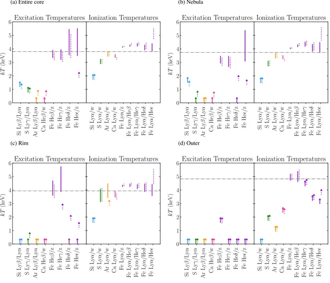
A line ratio of different transitions in the same ion reflects the kinetic temperature of free electrons in the plasma, and is

re-ferred to as “excitation temperature” orTe. Referring to Figure

4, we calculated theTefrom the observed line ratios of Lyβ/Lyα

of Si and Ar, Lyγ/Lyα of S, Heβ/w of Ca, and Heβ/z, Heγ/z, Heδ/z, and Heǫ/z of Fe (top three rows of Figure 4). S Lyβ is not used because it is not separated from Ar z, whose energy is 3102 eV (see Figure 3). Fe Lyβ is not used because of the

low observed flux. Fluxes of Lyα1and Lyα2were co-added in

this calculation. In the same manner, the fine structures of Lyβ, Lyγ, Heβ, Heγ, Heδ and Heǫ were also summed. The interval of the observed line ratios and the corresponding temperature ranges are overlaid on Figure 4 as color boxes.

Separately from the Tediagnostics, we used line ratios of

different ionization species to measure the ion fraction for each element. We parameterize these ratios by “ionization

temper-atures” orTZ. When the emission comes from a single

com-ponent and optically thin plasma under the CIE,TZfrom

ev-ery element should be the same asTe. TheTZ were

calcu-lated using the line ratios of Lyα/w of Si, S, Ar, and Ca and Lyα/z, Lyα/Heβ, Lyα/Heγ, Lyα/Heδ, and Lyα/Heǫ of Fe (bot-tom three rows of Figure 4). The temperature range derived from the observed line ratios are shown in Figure 4.

We summarize the derivedTeandTZin Figure 5. TZfrom

Fe, which is determined with the smallest statistical

uncertain-ties, has typical values of 4–5 keV.TZfrom the Entire core and

Nebula regions are clearly different among elements; namely

there is a tendency of increasing TZ with increasing atomic

number. These results indicate deviation from a single

temper-ature CIE model.TZfrom the Rim also suggests a slight

devia-tion from a single temperature model. The results of the Outer region are consistent with a single temperature approximation.

Tefrom Fe for the Nebula and Rim are about 3 and 4 keV,

respectively. In the Nebula and Entire core regions,Tefrom Fe

are lower thanTZat the 2–3σ level, providing further evidence

for deviation from the single temperature approximation. For

0 2 4 6 0.0 0.1 0.2 Si Lyβ/Lyα Si Lyβ/Lyα Si Lyβ/Lyα Si Lyβ/Lyα 0 2 4 6 0.000 0.025 0.050 S Lyγ/Lyα S Lyγ/Lyα S Lyγ/Lyα S Lyγ/Lyα 0 2 4 6 0.0 0.1 Ar Lyβ/Lyα Ar Lyβ/Lyα Ar Lyβ/Lyα Ar Lyβ/Lyα 0 2 4 6 0.0 0.1 0.2

L

in

e

F

lu

x

R

at

io

0 2 4 6 0.00 0.25 0.50 Fe Heβ/z Fe Heβ/z Fe Heβ/z Fe Heβ/z 0 2 4 6 0.0 0.1

0.2 Fe Heγ/zFe Heγ/zFe Heγ/zFe Heγ/z

0 2 4 6

0.00 0.05

0.10 Fe Heδ/zFe Heδ/zFe Heδ/zFe Heδ/z

0 2 4 6

Excitation Temperature (keV)

0.000 0.025 0.050 Fe Heǫ/z Fe Heǫ/z Fe Heǫ/z Fe Heǫ/z 0 2 4 6 0 5 10 Si Lyα/w Si Lyα/w Si Lyα/w Si Lyα/w 0 2 4 6 0.0 2.5 5.0 S Lyα/w S Lyα/w S Lyα/w S Lyα/w 0 2 4 6 0 2 4 Ar Lyα/w Ar Lyα/w Ar Lyα/w Ar Lyα/w 0 2 4 6 0.0 0.5 1.0 1.5

L

in

e

F

lu

x

R

at

io

0 2 4 6 0.0 0.5 1.0 Fe Lyα/z Fe Lyα/z Fe Lyα/z Fe Lyα/z 0 2 4 6 0 1 2 Fe Lyα/Heβ Fe Lyα/Heβ Fe Lyα/Heβ Fe Lyα/Heβ 0 2 4 6 0 2

4 Fe Lyα/HeγFe Lyα/HeγFe Lyα/HeγFe Lyα/Heγ

0 2 4 6

Ionization Temperature (keV)

0 5 10 Fe Lyα/Heδ Fe Lyα/Heδ Fe Lyα/Heδ Fe Lyα/Heδ 0 2 4 6 0 10 20 Fe Lyα/Heǫ Fe Lyα/Heǫ Fe Lyα/Heǫ Fe Lyα/Heǫ AtomDB v3.0.9 SPEXACT v3.03.00 Entire core Nebula Rim Outer

Fig. 4: Upper 8 panels show flux ratios of the emission lines as a function of the excitation temperature, calculated from AtomDB (black solid curve) and SPEXACT (gray dashed curve) assuming a single temperature CIE plasma. The lines used in the calculations are denoted in each panel. The color boxes show the ranges of the observed line ratios and the corresponding AtomDB temperatures at the1σ confidence level. Magenta, blue, cyan, and green correspond to the Entire core, Rim, Nebula, and Outer regions, respectively. When the ranges of the statistical errors of the observed line ratios are outside the models, 3σ lower limits are shown instead by the color arrows. Lower 9 panels are the same as the upper panels but for the ionization temperature.

(a) Entire core S i L y β /L y α S L y γ /L y α A r L y β /L y α C a H eβ /w F e H eβ /z F e H eγ /z F e H eδ /z F e H eǫ /z 0 1 2 3 4 5 6 k T (k eV ) Excitation Temperatures S i L y α /w S L y α /w A r L y α /w C a L y α /w F e L y α /z F e L y α /H eβ F e L y α /H eγ F e L y α /H eδ F e L y α /H eǫ Ionization Temperatures (b) Nebula S i L y β /L y α S L y γ /L y α A r L y β /L y α C a H eβ /w F e H eβ /z F e H eγ /z F e H eδ /z F e H eǫ /z 0 1 2 3 4 5 6 k T (k eV ) Excitation Temperatures S i L y α /w S L y α /w A r L y α /w C a L y α /w F e L y α /z F e L y α /H eβ F e L y α /H eγ F e L y α /H eδ F e L y α /H eǫ Ionization Temperatures (c) Rim S i L y β /L y α S L y γ /L y α A r L y β /L y α C a H eβ /w F e H eβ /z F e H eγ /z F e H eδ /z F e H eǫ /z 0 1 2 3 4 5 6 k T (k eV ) Excitation Temperatures S i L y α /w S L y α /w A r L y α /w C a L y α /w F e L y α /z F e L y α /H eβ F e L y α /H eγ F e L y α /H eδ F e L y α /H eǫ Ionization Temperatures (d) Outer S i L y β /L y α S L y γ /L y α A r L y β /L y α C a H eβ /w F e H eβ /z F e H eγ /z F e H eδ /z F e H eǫ /z 0 1 2 3 4 5 6 k T (k eV ) Excitation Temperatures S i L y α /w S L y α /w A r L y α /w C a L y α /w F e L y α /z F e L y α /H eβ F e L y α /H eγ F e L y α /H eδ F e L y α /H eǫ Ionization Temperatures

Fig. 5: Excitation temperatures and ionization temperatures derived from individual line ratios in (a) the Entire core, (b) Nebula, (c) Rim, and (d) Outer regions. Cyan, green, orange, pink, and purple indicate Si, S, Ar, Ca, and Fe, respectively. The results based on

AtomDB and SPEXACT are shown by the solid and dotted lines, respectively. The horizontal dash-dotted lines show the best-fitkTline

of the modified 1T model described in §3.2.1 and §3.3.

all consistent with the CIE prediction with the temperature of 2–4 keV within the statistical 1–2σ errors, however, the

corre-spondingTeare not constrained.

3.2 Modelling of the Broad-band Spectrum in the Entire Core Region

We then tried to reproduce the broad-band (1.8–20.0 keV) spectrum with optically-thin thermal plasma models based on AtomDB and SPEXACT. In the analysis of this section, we focused on the spectrum of the Entire core region in order to ignore the contamination of photons scattered due to the point spread func-tion (PSF) of the telescope, and to investigate uncertainties due to the atomic codes and the effective area calibration.

3.2.1 Single temperature plasma model

Although the SXS spectra indicate multi-temperature condi-tions, we begin by fitting the data with the simplest model, that is, a single temperature CIE plasma model (hereafter the 1CIE

model), with the temperature (kT1CIE), the abundances of Si, S,

Ar, Ca, Cr, Mn, Fe, and Ni, the line-of-sight velocity dispersion, and the normalization (N ) as free parameters. The abundances of other elements from Li through Zn were tied to that of Fe.

Since the resonance line of He-like Fe (FeXXVw) is subject to

the resonance scattering effect (see the RS paper), we replaced it by a single Gaussian so that it does not affect the parameters we obtained. The best-fit parameters are shown in Table 4; AtomDB

and SPEXACT give consistent temperatures of3.95 ± 0.01 keV

and3.94 ± 0.01 keV, respectively. The C-statistics are within

the expected range that is calculated according to Kaastra 2017, and hence the fits are acceptable even in these simple models.

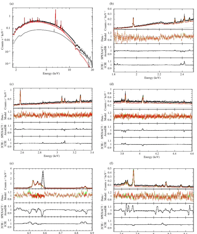
(a) 10 2 5 20 10−4 10−3 0.01 0.1 1 Counts s −1 keV −1 Energy (keV) (b) 0.1 0.2 0.3 0.4 Counts s −1 keV −1 0.8 1 1.2 Model Data / 0.9 1 1.1 AtomDB SPEXACT / 1.8 2 2.2 2.4 0.9 1 1.1 1CIE 2CIE / Energy (keV) (c) 0.5 1 Counts s −1 keV −1 0.8 1 1.2 Model Data / 0.9 1 1.1 AtomDB SPEXACT / 2.6 2.8 3 3.2 3.4 0.9 1 1.1 1CIE 2CIE / Energy (keV) (d) 0.2 0.4 0.6 0.8 1 Counts s −1 keV −1 0.8 1 1.2 Model Data / 0.9 1 1.1 AtomDB SPEXACT / 3.8 4 4.2 4.4 4.6 0.9 1 1.1 1CIE 2CIE / Energy (keV) (e) 1 2 3 4 Counts s −1 keV −1 0.8 1 1.2 Model Data / 0.9 1 1.1 AtomDB SPEXACT / 6.5 6.6 6.7 6.8 6.9 0.9 1 1.1 1CIE 2CIE / Energy (keV) (f) 0.1 0.2 0.3 0.4 0.5 Counts s −1 keV −1 0.8 1 1.2 Model Data / 0.9 1 1.1 AtomDB SPEXACT / 7.6 7.8 8 8.2 8.4 0.9 1 1.1 1CIE 2CIE / Energy (keV)

Fig. 6: The spectra in the Entire core region fitted with the modified-1CIE model. The entire energy band of 1.8–20.0 keV is shown in (a), and narrower energy bands of 1.8–2.5 keV, 2.5–3.4 keV, 3.7–4.6 keV, 6.4–6.9 keV, and 7.5–8.5 keV are shown in (b)–(f). The black solid curve is the total model flux, and the red and gray curves indicate the ICM component based on AtomDB and the AGN component, respectively. (b)–(f) include the green lines indicating the ICM component based on SPEXACT. The figure (e),

covering the 6.4–6.9 keV band, shows also the Gaussian (black dashed curve) which substitutes FeXXVw in the plasma model. All

the spectra are rebinned after the fitting just for display purposes. The second panels in (b)–(f) are the ratio of the data to the model of AtomDB (red) and SPEXACT (green). The third panels in (b)–(f) are the comparison of SPEXACT and AtomDB in the modified 1CIE model. The bottom panels in (b)–(f) shows the ratio of the 2CIE model to the modified 1CIE model based on AtomDB.

Table 3: Observed line fluxes derived from Gaussian fits.∗

Line name Flux (10−5ph cm−2s−1)

Entire Core Nebula Rim Outer SiXIIIw 6.40+4.71 −2.67 5.87+3.60 −2.54 <5.45 <4.54 SiXIVLyα1 32.43+2.29 −2.23 20.11+1.92 −1.83 21.83+2.64 −2.52 4.09+2.27 −1.72 SiXIVLyβ1 6.96+0.91 −0.87 5.03 +0.74 −0.70 3.93 +1.04 −0.98 1.21 +0.82 −0.58 SXVw 9.38+1.13 −1.11 7.26 +0.98 −0.99 3.91 +1.03 −0.94 <1.08 SXVILyα1 22.71 +0 .73 −0.72 15.81 +0 .64 −0.63 12.46 +0 .77 −0.76 2.70 +0 .67 −0.64 SXVILyβ1 3.83+0.29 −0.29 2.55 +0.25 −0.24 2.49 +0.35 −0.33 0.62 +0.27 −0.22 SXVILyγ1 1.20+0.20 −0.19 0.74 +0.15 −0.17 0.92 +0.25 −0.24 0.32 +0.22 −0.17 ArXVIIw 3.72+0.37 −0.36 2.82+0.31 −0.30 1.87+0.51 −0.47 1.20+0.41 −0.34 ArXVIIILyα1 5.47+0.29 −0.29 3.85+0.25 −0.25 3.15+0.32 −0.30 0.94+0.32 −0.30 ArXVIIILyβ1 0.77+0.15 −0.15 0.51 +0.12 −0.12 0.63 +0.20 −0.18 0.26 +0.15 −0.11 CaXIXw 5.20+0.27 −0.27 3.66 +0.23 −0.23 2.94 +0.30 −0.28 0.93 +0.29 −0.26 CaXIXHeβ1 0.66 +0.16 −0.10 0.46 +0.13 −0.10 0.67 +0.29 −0.35 0.21 +0.16 −0.12 CaXXLyα1 2.80 +0.18 −0.18 1.85 +0.16 −0.15 1.81 +0.20 −0.19 0.77 +0.20 −0.19 FeXXVw 33.14+0.43 −0.34 21.09+0.32 −0.31 22.13+0.49 −0.35 9.49+0.45 −0.44 FeXXVz 13.26+0.27 −0.25 8.72+0.21 −0.22 8.41+0.28 −0.27 3.03+0.28 −0.27 FeXXVHeβ1 4.73+0.12 −0.24 2.80 +0.12 −0.15 3.35 +0.19 −0.18 1.49 +0.21 −0.20 FeXXVHeβ2 1.04+0.10 −0.18 0.73 +0.14 −0.08 0.55 +0.13 −0.13 <0.17 FeXXVHeγ1 1.75 +0 .13 −0.13 1.04 +0 .10 −0.10 1.32 +0 .14 −0.13 0.25 +0 .13 −0.12 FeXXVHeδ1 0.88 +0.12 −0.12 0.55 +0.10 −0.10 0.63 +0.13 −0.12 0.27 +0.13 −0.11 FeXXVHeǫ1 0.54+0.10 −0.10 0.34+0.08 −0.08 0.43+0.12 −0.12 0.15+0.12 −0.10 FeXXVILyα1 3.68+0.16 −0.16 2.24+0.13 −0.13 2.68+0.17 −0.17 1.35+0.22 −0.21 FeXXVILyα2 2.17+0.14 −0.13 1.31+0.12 −0.11 1.59+0.14 −0.14 0.99+0.20 −0.18 FeXXVILyβ1 0.30+0.06 −0.06 0.21 +0.06 −0.05 0.18 +0.07 −0.04 0.16 +0.08 −0.06 NiXXVIIw 1.43+0.13 −0.13 1.01 +0 .11 −0.11 0.79 +0 .13 −0.13 0.43 +0 .16 −0.15 ∗_{The Lyα}

2lines of Si, S, Ar, and Ca are not shown because their parameter values

are tied to Lyα1(see Table 2 for details).

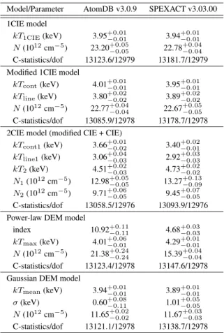
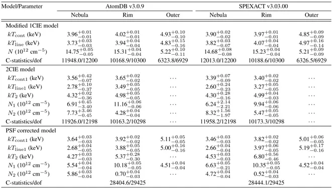
Table 4: Best fit parameters for the Entire core region Model/Parameter AtomDB v3.0.9 SPEXACT v3.03.00 1CIE model kT_{1CIE(keV) 3.95}+0.01 −0.01 3.94 +0.01 −0.01 N (1012_cm−5_{) 23.20}+0.05 −0.05 22.78 +0.04 −0.04 C-statistics/dof 13123.6/12979 13181.7/12979 Modified 1CIE model

kT_cont(keV) 4.01+0.01_−0.01 3.95+0.01_−0.01 kT_{line(keV) 3.80}+0.02 −0.02 3.89 +0.02 −0.02 N (1012_cm−5_{) 22.77}+0.04 −0.04 22.67 +0.05 −0.05 C-statistics/dof 13085.9/12978 13178.7/12978 2CIE model (modified CIE + CIE)

kT_cont1(keV) 3.66+0.01_−0.02 3.40+0.02_−0.01 kT_line1(keV) 3.06+0.04 −0.03 2.92 +0.03 −0.03 kT_{2(keV) 4.51}+0.02 −0.03 4.73 +0.02 −0.02 N₁(1012_cm−5_{) 12.98}+0.05 −0.05 13.27 +0.13 −0.09 N₂(1012_cm−5_{) 9.71}+0.06 −0.05 9.45 +0.07 −0.05 C-statistics/dof 13058.5/12976 13093.9/12976 Power-law DEM model

index 10.92+0.11_−0.11 4.68+0.03_−0.03 kTmax(keV) 4.01+0.06_−0.01 4.29+0.01_−0.01 N (1012_cm−5_{) 21.38}+0.24 −0.24 15.39 +0.04 −0.04 C-statistics/dof 13123.4/12978 13147.6/12978 Gaussian DEM model

kT_{mean(keV) 3.94}+0.01 −0.01 3.89 +0.01 −0.01 σ (keV) 0.60+0.08_−0.11 1.01+0.05_−0.05 N (1012_cm−5_{) 11.65}+0.02 −0.02 11.67 +0.03 −0.03 C-statistics/dof 13121.1/12978 13138.7/12978 3.8 4.0 4.2 k T (k eV ) kTcont1 kTline1

ARFnormalARFground ARFCrab ARFnormal ARFground ARFCrab

12900 13000 13100 13200 13300 C -s ta ti st ic s ——– AtomDB 3.0.9 ——– —— SPEXACT 3.03.00 ——

Fig. 7: Comparison of the best-fit temperatures and C-statistics among different ARFs and atomic databases for the modified 1CIE model.

In the 1CIE fit, both the continuum shape and the emission-line fluxes participate in the temperature determination. In or-der to fully utilize the line resolving power of the SXS, we then modeled the continuum and lines separately and

deter-mined the continuum temperatures (kTcont) and the line

tem-peratures (kTline) (hereafter the modified 1CIE model). In this

model,kTcontandkTlinewere independently allowed to vary

whereas the other parameters were common (implemented as the bvvtapec model in Xspec). The best-fit parameters we ob-tained are shown in Table 4. Both AtomDB and SPEXACT pro-vide a reasonably good fit to the observed spectrum as shown

in Figure 6. Compared tokT1CIE, kTcontandkTline become

slightly higher and lower, respectively, for both AtomDB and

SPEXACT. Since kTcont is closer to kT1CIE than kTline, the

continuum shape most likely determines the temperature of the 1CIE model, rather than the line fluxes, even with high-resolution spectroscopy measurements. The temperature differ-ences between AtomDB and SPEXACT are formally statistically significant, but are less than 0.1 keV.

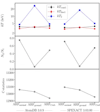
The difference between kTcont and kTline is at most

0.23 keV but statistically significant. As we found the multi-temperature structure from the line ratio diagnostics (§3.1), that difference is possible. However, an uncertainty in the effec-tive area also might affects the results; the in-flight calibration of Hitomi was not completed because of its short life time. We therefore assessed this uncertainty using the modified ARF

based on the ground telescope calibration (ARFground) and the

actual Crab data (ARFCrab). See Appendix 4 for the detailed

correction method. We fitted the modified 1CIE model using ARFground and ARFCrab. The correction of the ARF slightly affects the parameters of the AGN components as well (see Table 4 of the AGN paper). Even though the differences are very small, we used the specific AGN parameter values

cor-2 5 10 20 k T (k eV ) kTcont1 kTline1 kT2 0.0 0.2 0.4 0.6 0.8 N2 /N 1

ARFnormal ARFground ARFCrab ARFnormal ARFground ARFCrab

12900 13000 13100 13200 13300 C -s ta ti st ic s ——– AtomDB 3.0.9 ——– —— SPEXACT 3.03.00 ——

Fig. 8: Comparison of the best-fit temperatures and C-statistics among different ARFs and atomic databases for the 2CIE model.

responding to each assumed ARF in our fits. The temperatures

and C-statistics we obtained are summarized in Figure 7.kTcont

varies depending on ARF because the continuum shape is sub-ject to the effective area shape. On the other hand, the values

ofkTline measured with different assumptions for the ARF

re-main consistent with each other. Therefore,kTlineprovides the

most robust estimate of the temperature from the SXS spectrum assuming a single-phase model. In terms of the C-statistics, the

ARFCrabgives the best-fit, but this choice of ARF also results

in the largest difference betweenkTcont andkTline. This

illus-trates the difficulty of effective area calibration with the limited amount of available data.

Even though the AGN paper carefully modeled the AGN emission, the uncertainty of its model parameters and their im-pact on the best-fit temperature structure should also be

consid-ered. If the AGN model is slightly changed,kTcontwould again

change, whilekTlinewould be less affected as demonstrated in

the comparison of the ARFs.

3.2.2 Two temperature plasma models

The line ratio diagnostics in §3.1 actually indicate the presence of multi-temperature structure in the Perseus cluster core. As a simple approximation of the deviations from a single thermal phase, we first used a two-temperature model where another CIE model was added to the modified 1CIE model (hereafter the 2CIE model). The free parameters of the additional CIE

component were the temperature and the normalization, while the abundances and the line-of-sight velocity dispersion were tied to those of the primary component. The results are shown in Table 4. As expected, the C-statistics are significantly im-proved from those of the modified 1CIE model (∆C = 30–91). However, as shown in the bottom panels of Figure 6 (b)–(f), the continuum is almost the same and the difference of line emissiv-ities are at most 10% compared to the 1CIE model. The temper-atures and normalizations obtained with the two spectral codes are in reasonably good agreement, although some differences are statistically significant. The dominant component now has

a temperature ofkTline= 3.06 ± 0.03 keV from AtomDB, which

is fully consistent withkTline= 3.06+0.03_−0.08keV from SPEXACT.

The second thermal component is from hotter gas withkT2∼5

keV; for this component, SPEXACT gives a ∼10% higher

tem-perature than AtomDB, and a somewhat lower relative

normal-ization (N2/(N1+ N2) of 31% with SPEXACT and 43% with

AtomDB). The temperatures derived from the 2CIE fit are con-sistent with the line ratio diagnostics shown in Figure 5; the

ion-ization temperature of S is ∼3 keV and that of Fe is ∼ 4.5 keV.

We also checked difference of the line-of-sight velocity disper-sion between the lower and higher temperature components, but no significant difference was found (see Appendix 5 for details). In the same manner as for the modified 1CIE model (§3.2.1),

we examined the effect of different ARFs (ARFground and

ARFCrab) for the 2CIE model. Figure 8 shows the resulting

temperatures, the ratio of the normalizations (N2/N1), and the

C-statistics for each ARF. The best-fit parameter values vary significantly depending on the choice of ARF, but the

temper-atures of ARFnormaland ARFCrabare very close to each other

(∼3 keV plus ∼5 keV). Only ARFgroundshows the presence of

a>20 keV component, which seems physically less well

moti-vated. The different trend in ARFgroundis likely caused by an

incomplete modeling of the continuum; as shown in the mid-dle panel of Figure 16 (Appendix 4), downward convex

resid-uals are seen in the 2–7 keV band for ARFground. In any case,

the trend where the dominant component has a temperature of 3–4 keV and the sub-dominant additional phase has a higher temperature, is robust.

3.2.3 Other combinations of collisional plasma models We also tried to add one more CIE component to the 2CIE model (i.e., 3CIE model), but no significant improvements of the C-statistics are found. Therefore, the 2CIE model is suffi-cient to reproduce the observed spectrum.

The actual temperature structure of the ICM might not con-sist of discrete temperature components but rather of a contin-uous temperature distribution. Indeed, some hints of a power-law or a Gaussian temperature distributions were reported in the literature (e.g., Kaastra et al. 2004; Simionescu et al. 2009). We therefore applied these simple differential emission

sure (DEM) models to the SXS spectrum. The emission

mea-sure profile, EM (kT ), is proportional to (kT /kTmax)

α for

the power-law DEM model and toexp(−(kT − kTmean)2/2σ)

for the Gaussian DEM model. The best-fit parameters of the models are summarized in Table 4. Both the power-law and the Gaussian DEM models show steep temperature

distribu-tions peaked at ∼4 keV, even though the distributions based

on SPEXACT are slightly wider (smaller index or largerσ) than

those based on AtomDB. In any case, we found no significant im-provements from the 2CIE model. Further investigation of the multi-temperature model is shown in Section 3.4 and Figure 10. Another possible cause of the deviation from a single tem-perature model shown in the line ratio diagnostics is the NEI

state, which is often observed in supernova remnants. We

thus tried to fit the spectrum with a NEI model (the possibil-ities of both an ionizing and a recombining plasma are con-sidered). However, the obtained ionization parameter becomes

nt > 1×1012_cm−3_s−1_{, and the temperature is almost the same}

as the 1T model; therefore the model is consistent with a CIE state, and we find no significant signature of the NEI.

3.3 Spatial Variation of the Temperature Structure We next modeled the broad-band spectra in the Nebula, Rim, and Outer regions in order to look for spatial trends in the tem-perature distribution. The fit results obtained with the modified 1CIE model are shown in the top rows of Table 5. Compared to the result from the Entire core region, the temperature in the Nebula region is slightly lower, while that in the Rim region is slightly higher. The temperature continues to increase at larger radii, reaching 5 keV in the Outer region. These results are con-sistent with the temperature map obtained from XMM-Newton and Chandra observations (Churazov et al. 2003; Sanders & Fabian 2007).

The line ratio diagnostics show a deviation from the single temperature approximation in the Nebula and Rim regions. We thus applied the 2CIE model to the spectra of those regions. The best-fit parameters are also shown in the middle rows of Table 5. The C-statistics were improved from the modified 1CIE model (∆C = 6–59). Both the Nebula and Rim regions show the same composition as the Entire core (roughly 3 keV plus 5 keV), but with different normalization ratios (the relative contribution of the hotter component is lower in the Rim re-gion, although significant differences between the two spectral codes are also found). Large asymmetrical errors of the nor-malizations in the Nebula region are likely due to the compara-ble normalization values of the two components and the limited energy band (> 1.8 keV). In the Nebula region, the

discrep-ancy betweenkTcontandkTlinebecomes large (∼1.0 keV), and

kTline shows the lowest temperature of ∼2.7 keV among the

different spatial regions considered. We also checked the 2CIE

model in the Outer region, but no improvements from the mod-ified 1CIE model were found (∆C < 1), as expected from the line ratio diagnostics. The systematic uncertainty of the tem-perature measurements due to the different ARFs has a similar trend as the analysis of the Entire core region (see Appendix 4). The sizes of the regions used for spatially resolved spec-troscopy are comparable to the angular resolution of the tele-scope. Therefore, photons scattered from the adjacent regions due to the telescope’s PSF tail might affect the fitting results. We calculated the expected fraction of scattered photons with ray-tracing simulations, and show the results in Table 6; the fractions reach up to 30%, and are not negligible. We thus per-formed a “PSF corrected” analysis, in which all the regions were simultaneously fitted taking into account the expected fluxes of photons scattered between regions. We used the 2CIE model for the Nebula and Rim regions and the 1 CIE model for the Outer region according to the results presented above. The best-fit parameters of the PSF corrected model are shown in the bottom rows of Table 5. After the PSF correction, the ratios of the normalizations are changed but the temperatures we ob-tained are almost consistent with those derived from the PSF “uncorrected” analysis.

3.4 Comparison with Multi-temperature Models from Previous Observations

Chandra/ACIS and XMM-Newton/RGS observations revealed a multi-temperature structure ranging between 0.5–8.0 keV in the core of the Perseus cluster (Sanders & Fabian 2007; Pinto et al. 2016). Here we use a similar multi-temperature analysis to check the consistency between Hitomi/SXS and these previous measurements.

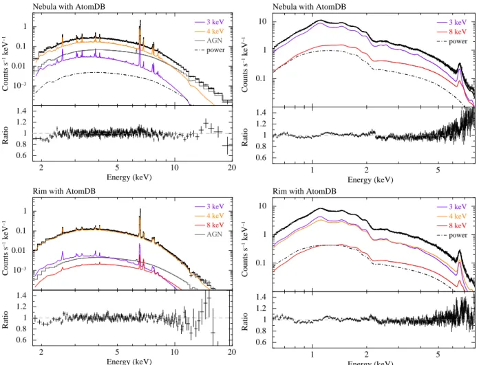
We fitted the SXS spectra extracted from the Nebula and Rim regions with a six-temperature CIE model consisting of 0.5 keV, 1 keV, 2 keV, 3 keV, 4 keV and 8 keV components fol-lowing Sanders & Fabian (2007). The temperature of each com-ponent was fixed, and the abundance and line-of-sight velocity dispersion were common to all the components. The power-law component that was found in Sanders & Fabian (2007) and interpreted as a possible inverse-Compton emission was also

in-cluded in our model with a fixed photon index ofΓ = 2. The

spectra and the best-fit models in the Nebula and the Rim re-gions are shown in the left column of Figure 9. The normaliza-tions we obtained for each temperature were scaled to sum to unity, and the results are plotted in Figure 10 as red diamonds. The profile of the scaled normalizations are very similar be-tween AtomDB and SPEXACT, except for the 8 keV component which is detected with SPEXACT in both the Nebula and Rim re-gions while only its upper limit was obtained for AtomDB. The results indicate that the combination of the 3 keV, 4 keV, and 8 keV components approximates the 2CIE model obtained in