Department of Electronics, Informatics and Bioengineering
p o l i t e c n i c o d i m i l a n o
m a n ua l e
d i c o r p o r at e i d e n t i t y
m i l a n o, m ag g i o 2 0 1 5BWaveR: an FPGA-accelerated
Genomic Sequence Mapper
Leveraging Succinct Data Structures
NECSTLab
Novel, Emerging Computing System Technologies Laboratory Politecnico di Milano
Advisor: Prof. Marco D. Santambrogio Politecnico di Milano
Co-advisor: Dott. Ing. Lorenzo Di Tucci Politecnico di Milano
Master Thesis of:
Guido Walter Di Donato - 897749
Do I contradict myself ? Very well, then, I contradict myself ; I am large - I contain multitudes . Walt Whitman
First, I would like to say thanks to my advisor, Marco Domenico Santambrogio, for being a role model and a friend, and for giving me the opportunity to work on this amazing project. Without his guidance, support, and critical thinking towards my work, this thesis would never have been possible.
Also, I would like to thank all the people working in the NECSTLab for cre-ating a friendly, stimulcre-ating, and challenging environment sharing expertise and suggestions. I am very thankful to Lorenzo, who introduced me to the world of genomics and bioinformatics, and followed with interest the development of this work. Huge thanks also to Alberto, not only for giving me lots of useful insights about FPGAs and the tools for programming them, but also, and foremost, for being a great friend.
I am grateful to all the friends I met in these years, who made my journey at Politecnico a wonderful experience. Special thanks to Simone, Alessia, and Marco: I will remember forever the happy time we spent together.
I also want to say thanks to my beautiful and extraordinary family. Despite being far away, all of you always found a way to be by my side and to make me feel at home, wherever I was.
iii
Last but foremost, my biggest thank you goes to my lovely parents, Salvatore and Giovanna, and to my “little” brother, Andrea: you are my inspiration and my motivation. Without the trust, the support, and the encouragement you have al-ways given to me, I might not be the person I am today. I could not have achieved any of this without you.
T
he advent of Next Generation Sequencing (NGS) produced an explosion in the amount of genomic data generated, which resulted in the birth and early development of personalized medicine. However, the tools currently employed for the analysis of these data still require too much time and power. Thus, to boost the research in this field, new bioinformatic tools are needed, which can efficiently handle the vast amount of genomic data, in order to keep up with the pace of NGS technologies. In this scenario, the aim of this thesis is the design and the implementation of a memory-efficient, easy-to-use short sequence mapper, to be employed in various bioinformatic applications. At the core of the proposed tool there is an efficient implementation of a succinct data structure, allowing to compress the genomic data while still providing efficient queries on them. A comprehensive description of the data encoding scheme is presented in this work, together with the characterization of the proposed data structure in terms of memory utiliza-tion and execuutiliza-tion time.To improve the performances and the energy efficiency of the sequence map-ping process, this thesis also proposes a custom hardware design, which lever-ages the compression capability of the proposed data structure to fully exploit the
v
highly parallel architecture of Field Programmable Gate Arrays (FPGAs). We em-ployed such custom hardware architecture to develop BWaveR, a fast and power-efficient hybrid sequence mapper, which is made available through an intuitive web application that guarantees high usability and provides great user experience. Finally, this work provides a validation of the developed tool, in order to prove the correctness and reliability of the results it produces. Moreover, we present an extensive evaluation of the performances of the proposed hybrid system, through a comparison with state-of-the-art equivalent software tools. The experimen-tal results show that the proposed hardware architecture is able to provide ap-plication speed-up while significantly reducing the energy consumption. Thus, BWaveR constitues a valid solution for accelerating bioinformatic applications involving genomic sequence mapping, allowing users to benefit from hardware acceleration without any development effort or any knowledge of the underlying hardware architecture.
L
o sviluppo di tecnologie di sequenziamento sempre più effici-enti, che prendono il nome di Next Generation Sequencing (NGS), ha portato ad un rapidissimo aumento della quantità di dati ge-nomici disponibili, ponendo le basi per la nascita della medicina personalizzata. Purtroppo però, l’analisi di una tale quantità di dati richiede, ad oggi, ancora troppo tempo e troppa energia. Nuovi strumenti computazionali sono quindi necessari per accelerare la ricerca in questo campo, e per garantire lo sviluppo e la democratizzazione della medicina personalizzata.In tale contesto, lo scopo di questa tesi è la progettazione e la realizzazione di un tool per l’allineamento di sequenze genomiche, che risulti efficiente e facile da utilizzare in diverse applicazioni bioinformatiche. Il funzionamento di tale tool è basato su una struttura dati succinta, che permette di comprimere efficace-mente i dati genomici, riducendo l’utilizzo di memoria e permettendo, allo stesso tempo, un rapido accesso a tali dati. In questo elaborato verrà fornita un’ampia descrizione della struttura dati proposta, del suo utilizzo, e delle sue caratteris-tiche in termini di utilizzo di memoria e tempi d’esecuzione.
Questa tesi presenta anche la realizzazione di BWaveR, un sistema eterogeneo per l’allineamento di sequenze, che si avvale delle ridotte dimensioni della
vii
tura dati proposta per sfruttare al meglio l’architettura parallela dei Field Pro-grammable Gate Arrays (FPGAs). Tali dispositivi offrono vantaggi significativi dal punto di vista dell’efficienza energetica, ma risultano particolarmente difficili da programmare. BWaveR, invece, consente di sfruttare i vantaggi dell’accelerazione hardware attraverso una semplice ed intuitiva applicazione web, che garantisce un facile utilizzo ed una buona user experience.
Il tool sviluppato è stato validato e valutato attreverso il confronto con ap-plicativi software equivalenti. I test di validazione dimostrano l’affidabilità di BWaveR e provano la consistenza dei risultati prodotti. Inoltre, i risultati sper-imentali mostrano che l’architettura hardware proposta è in grado di ridurre il tempo d’esecuzione ed il consumo energetico del processo di allineamento di se-quenze genomiche. Pertanto, BWaveR si propone come una valida soluzione per accelerare una vasta gamma di applicazioni bioinformatiche, permettendo anche ad utenti senza competenze di programmazione di beneficiare dei vantaggi di un’architettura hardware specializzata.
Contents viii
List of Figures xi
List of Tables xiii
List of Algorithms xiv
List of Abbreviations xv 1 Introduction and motivation 1
1.1 Thesis goal . . . 4
1.2 Outline . . . 5
2 Background 6 2.1 Genome sequencing . . . 6
2.2 Genome assembly . . . 11
2.2.1 De novo genome assembly . . . 12
2.2.2 Comparative genome assembly . . . 16
2.3 Genomic analysis . . . 17
Contents ix
3 Problem Description 21
3.1 Genomic sequences: FASTA and FASTQ file format . . . 21
3.2 Burrows-Wheeler Mapping . . . 23
3.3 Succinct Data Structures . . . 27
3.3.1 Wavelet Tree . . . 29
3.3.2 RRR Data Structure . . . 30
3.4 Hardware Accelerators . . . 32
4 Related work 36 4.1 Read alignment and Burrows-Wheeler mapping . . . 36
4.2 Hardware implementations . . . 41
4.2.1 GPU-based implementations . . . 42
4.2.2 FPGA-based implementations . . . 43
4.3 Usability of the alignment tools . . . 46
4.4 Summary . . . 51
5 Proposed solution: Design & Implementation 53 5.1 Outline of the proposed sequence mapper . . . 54
5.2 Software implementation . . . 58
5.3 Hardware implementation . . . 70
5.4 BWaveR web application . . . 76
6 Experimental Evaluation 81 6.1 Experimental setup and design . . . 82
6.2 Validation . . . 85
6.4 Execution time . . . 87 6.5 Hardware implementation . . . 91
7 Conclusions and Future Work 94
7.1 Future Work . . . 96
List of Figures
2.1 The Sanger chain termination method for DNA sequencing . . . 8
2.2 Carlson curve: total cost of sequencing a human genome over time . 9 2.3 Shotgun sequencing overview . . . 10
3.1 Burrows-Wheeler Transform and Suffix Array construction . . . 25
3.2 The backward pattern matching procedure . . . 26
3.3 Wavelet tree of the sequence TTGGATAACCCC$G . . . 29
3.4 A rank query on the wavelet tree . . . 31
3.5 FPGA overview . . . 34
3.6 A logic block . . . 34
4.1 Bowtie2 command-line user interface . . . 48
4.2 BLAST web-based user interface . . . 49
5.1 Outline of the proposed sequence mapper . . . 55
5.2 BWaveR sequence mapper: overall work-flow . . . 56
5.3 BWaveR output file format: an example . . . 57
5.4 Optimized BWT and suffix array computation via de Bruijn graph . 60 5.5 Overview of the BWaveR data structure . . . 62
5.6 Overview of the implemented RRR sequence . . . 66
5.7 Schematic of the hardware design . . . 73
5.8 Example of reduction: sum of array elements . . . 75
5.9 Overview of the BWaveR web application . . . 77
5.10 BWaveR web app: Home Page . . . 77
5.11 BWaveR web app: Sequences Uploader page . . . 78
5.12 BWaveR web app: Results Downloader page . . . 79
6.1 Simple schematic of Xilinx Alveo U200 board . . . 83
6.2 Data structure’s size for E.Coli (left) and Human Chr.21 (right) . . . 86
6.3 Succinct encoding time for E.Coli (left) and Human Chr.21 (right) . 88 6.4 Reads mapping time for E.Coli . . . 89
List of Tables
6.1 Data structure’s size for E.Coli (Bytes) . . . 86
6.2 Data structure’s size for Human Chr.21 (Bytes) . . . 86
6.3 Succinct encoding time for E.Coli (sec) . . . 88
6.4 Succinct encoding time for Human Chr.21 (sec) . . . 88
6.5 Performances of BWaveR and Bowtie2 when mapping 100 millions 100bp reads to E.Coli reference. . . 92
6.6 Performances of BWaveR and Bowtie2 when aligning 1, 10 and 100 millions 100bp reads to Chr.21 reference. . . 93
1 Backward search algorithm . . . 28
2 Binary rank function on RRR sequences . . . 67 3 Backward search algorithm with succinct data structures . . . 69
List of Abbreviations
A Adenine. 7, 30, 64
API Application Programming Interface. 71, 91 ASIC Application Specific Integrated Circuit. 32, 33 BAM Binary Alignment Map. 57, 58
BLAST Basic Local Alignment Search Tool. 4, 50
bp base pairs. 10, 11, 27, 40, 44, 57, 73, 74, 84, 87, 89, 92, 96 BRAM Block Random Access Memory. 44, 73, 75, 92 BWA Burrows-Wheeler Aligner. 38–42, 45
BWT Burrows-Wheeler Transform. 3–5, 21, 24, 38, 40–43, 51–55, 58–64,
67, 68, 72, 73, 75, 79, 87, 91, 92
C Cytosine. 7, 64
CPU Central Processing Unit. 4, 32, 42–45, 54, 55, 71, 72, 91 DAWG Directed Acyclic Word Graph. 39
ddNs dideoxynucleotides. 7
DNA DeoxyriboNucleic Acid. 1, 2, 6–10, 12, 17, 19, 21, 22, 96 DP Dynamic Programming. 2, 37–40, 51, 96
DRAM Dynamic Random Access Memory. 73 DSP Digital Signal Processor. 35
FPGA Field Programmable Gate Array. 4, 5, 20, 21, 33, 35, 40, 41, 43–46,
51–55, 63, 70–74, 80, 82, 90–93, 95, 96
G Guanine. 7, 64
GPU Graphical Processing Unit. 33, 41–43, 45 GUI Graphic User Interface. 76
HGP Human Genome Project. 7 HLS High-Level Synthesis. 35, 71, 75 HTS High Throughput Sequencing. 8
IGSR International Genome Sample Resource. 84 LUT Look-Up Table. 33
MEM maximal exact matching. 38, 40 MUX multiplexer. 33
List of Abbreviations xvii
NCBI National Centre for Biotechnology Information. 22 NGS Next Generation Sequencing. 1, 2, 8, 9, 13, 14, 16, 41, 94 OLC Overlap-Layout-Consensus. 13–15
PC Personal Computer. 54 PE Processing Element. 46 RNA RiboNucleic Acid. 22, 64
RRR Raman, Raman and Rao. 4, 21, 29–31, 41, 51, 54, 63, 64, 66–68, 71, 72,
74, 91, 95
SA Suffix Array. 54, 58–61, 68, 79 SAM Sequence Alignment Map. 57, 58
SDSL Succinct Data Structures Library. 40, 63 SIMD Single Instruction Multiple Data. 39 SIMT Single Instruction Multiple Thread. 42 SLD System-Level Design. 35
SMEMs supermaximal exact matches. 40 SNP Single Nucleotide Polymorphism. 19 SRAM Static Random Access Memory. 33 T Thymine. 7, 64
U Uracile. 64
CHAPTER
1
Introduction and motivation
P
recision medicine holds promise for improving many aspects of health and healthcare. This emerging approach for disease treat-ment and prevention takes into account individual variability in genes, allowing doctors to predict, among different possible treat-ments, which is best suited to each individual or group of people. It is in contrast to the common one-size-fits-all approach, in which disease treatment and preven-tion strategies are developed for the average person, with less considerapreven-tion for the differences between individuals [1].One of the most promising fields of application of precision medicine is oncol-ogy. Clinicians and scientists are using Next Generation Sequencing (NGS) tools to gain insight into each patient’s disease, and treating cancer at the genomic level is having a profound impact on cancer care [2]. By examining the DeoxyriboNu-cleic Acid (DNA) of a patient’s tumor, it is possible to identify the cancer-causing genes that make it grow. This information allows researchers to find a drug that targets that gene, in order to deactivate it and attack the cancer cells [3].
Twenty years ago, gene sequencing cost millions and took months to receive results. With current technology instead, it is possible to do the sequencing and its interpretation at a reasonable cost, getting this information back to the patient and the patient’s doctor within a few weeks [3]. Thanks to the development of NGS tools, the actual sequencing of the DNA now takes only minutes and costs less than 1000$ per whole human genome. The complexity comes from “read-ing” the produced data in order to identify the abnormal genes patterns, which requires two main steps: genome assembly and genomic analysis.
Genome assembly (or sequence assembly) refers to merging sequenced DNA fragments, called “reads”, in order to reconstruct the original longer sequence they generated from [4]. Genomic analysis instead is the identification, mea-surement, and comparison of genomic features, followed by their annotation, that describes the function of the product of the identified genes [5]. Both these steps are computationally intensive and they share the same bottleneck: sequence alignment, defined as the arrangement of two or more nucleotide (or amino acid) sequences so that their most similar elements are juxtaposed [6]. Various ap-proaches can be found in the literature to address different formulations of the sequence alignment problem, that can be a global alignment [7], a local alignment [8] or a hybrid version of the problem, often referred as semi-global or glocal align-ment [9].
Many of the proposed approaches rely on Dynamic Programming (DP), an optimization method over plain recursion, which involves storing the results of sub-problems so that it is not necessary to re-compute them when needed later. Although this method allows reducing time complexities from exponential to polynomial, the amount of data to be processed is so vast that other optimizations
Introduction and motivation 3
are needed to further reduce the execution time. For this reason, many state-of-the-art sequence aligners rely on the seed and extend paradigm, consisting in finding exact matches between seeds (very short genomic subsequences), then extending the alignment in the selected regions through a dynamic program-ming approach [10]. Burrows-Wheeler Mapping is one of the most employed techniques for the exact matching of sequences, thus is often employed for the seeding step [11, 12]. It relies on the Burrows-Wheeler Transform (BWT) of the genomic sequence and its FM-index, that allow to efficiently carry out a backward search of a pattern within a large sequence.
In the last years, hardware accelerators proved to be effective in reducing the computation time of sequence alignment algorithms [13], and in optimizing the performance over power consumption ratio [14]. This is fundamental for de-creasing the cost of genome assembly and genomic analysis, and it is crucial for promoting the development and the diffusion of precision medicine. However, hardware accelerators are usually expensive and difficult to program. For this rea-son, a recent trend in bioinformatics is using hardware accelerators as a service, through cloud-based platforms which allow users to easily exploit the computa-tional power of the accelerators, without the need of buying and programming them [15].
Moreover, because of the vast amount of data to be processed, a noticeable effort has been put by researchers in representing the data in the most compact way. Here is where Succinct Data Structures come into play: these structures provide the possibility to encode genomic data in a space close to theoretical lower bound, while still allowing for fast queries on the data [16].
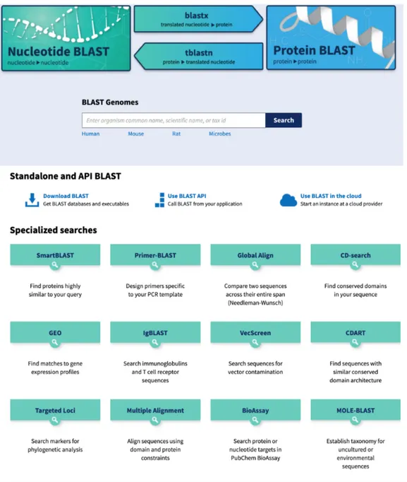
through command line interfaces, which limit their usability. A user-friendly easy-to-use interface is a key factor in determining the potential diffusion of a tool and its acceptance level in the bioinformatic community [17]. A famous example is the Basic Local Alignment Search Tool (BLAST), that thanks to its intuitive web-based graphical user interface is the most employed bioinformatic tool ever, with more than 75000 citations in published research papers [18].
1.1
Thesis goal
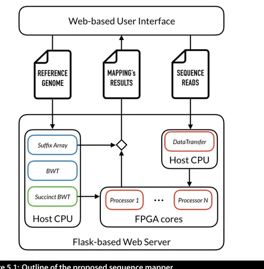
Considering all the aforementioned reasons, the aim of this work is the imple-mentation of a memory-efficient and easily accessible Burrows-Wheeler mapper, leveraging Field Programmable Gate Arrays (FPGAs) for improving the perfor-mance over power ratio of the mapping process. The proposed heterogeneous system exploits the general purpose Central Processing Unit (CPU) for the com-putation of the Burrows-Wheeler Transform of the reference genome, while the pattern matching (i.e. read mapping) is executed on FPGA. The CPU is also employed for encoding the BWT in a succinct data structure, and for the mem-ory management. Query sequences and their reverse complement are efficiently mapped to the reference genome, leveraging the high parallelism and the effi-cient bit-level operations of the FPGA architecture, to reduce the computation time and the energy consumption.
The reference genomic sequence, of length N , is encoded in a succinct data structure based on Wavelet Trees and Raman, Raman and Rao (RRR) structures, allowing fast rank and select queries on the BWT. Such succinct representation allows to efficiently perform pattern matching on the reference sequence, without
1.2. Outline 5
the need of storing any additional data. Actually, the implemented data structure is even able to compress the size of the data w.r.t. the original representation of the sequence, reducing the required space to∼ N
4 bytes, while still permitting to
search a pattern of length p in O(p) time, regardless of the reference’s size. The user-friendly web-based interface allows a user to upload the reference genome and the set of reads to be aligned, either in compressed or uncompressed FASTA/FASTQ format. A simple click triggers the computation of the BWT, its encoding in the succinct data structure, and finally the read alignment on FPGA. Thus, the user will get back his/her results without any effort, and without any knowledge of the underlying hardware architecture.
1.2
Outline
The remainder of the document is organized as follow. Chapter 2 will give some insights about genome sequencing, genome assembly, genomic analysis, and the importance of read alignment for the development of precision medicine. Chap-ter 3 will present the Burrows-Wheeler mapping problem, and the maChap-terials and methods employed in the development of the proposed tool. Continuing, Chap-ter 4 will discuss the state-of-the-art Burrows-Wheeler aligners, and it will present related works on hardware accelerators. Chapter 5 will give a detailed description of the proposed hybrid aligner and of its implementation, while Chapter 6 will present the experimental setup and the obtained results. Finally, Chapter 7 will draw the conclusions and possible future development of the proposed tool.
CHAPTER
2
Background
T
his Chapter introduces the reader to the genome assembly pro-cess and the genomic analysis, which are at the core of person-alized medicine. Section 2.1 describes the techniques employed for digitalizing the information contained in DNA, and the frag-mented data they produce. Then, Section 2.2 provides a description of the assem-bly approaches for creating a representation of the original chromosomes from which the DNA originated. Finally, Section 2.3 presents the applications of se-quence alignment for genome analysis and their central role in the development of precision medicine.2.1
Genome sequencing
DNA sequencing is the process of determining the sequence of the four chem-ical building blocks, called nucleotide bases, that make up a molecule of DNA. The double helix structure, characteristic of the DNA molecule, is due to the fact
2.1. Genome sequencing 7
that the four chemical bases bind in accordance with what is called “scheme of complementarity of the bases”: Adenine (A) always binds to Thymine (T), while Cytosine (C) always binds to Guanine (G). The scheme of complementarity is the basis for the mechanism by which DNA molecules are copied during meiosis, and the pairing also underlies the methods by which most DNA sequencing experi-ments are done [19]. Today, with the right equipment and materials, sequencing a short piece of DNA is relatively straightforward. However, Whole Genome Se-quencing (WGS), that is the process of digitalizing the complete DNA sequence of an organism’s genome at a single time, still remains a complex task. It requires breaking the DNA of the organism into many smaller pieces, sequencing them all, and assembling the resulting short sequences into a single long “consensus sequence”.
The Human Genome Project (HGP), an international collaborative research program, led to the completion of the first human genome in 2003, after about 15 years of effort [20]. In this project, DNA regions up to about 900 base pairs in length were sequenced using a method called Sanger sequencing or chain ter-mination method, developed by the British biochemist Frederick Sanger in 1977 [21]. Sanger sequencing is based on the iterative selective incorporation of chain-terminating dideoxynucleotides (ddNs) by DNA polymerase during in vitro DNA replication; ddNs may be radioactively or fluorescently labeled for detection in automated sequencing machines. An overview of the chain termination method is given in Figure 2.1; a comprehensive explanation of the method can be found in [21].
Sanger chain termination method gives high-quality sequences and it is still widely used for the sequencing of individual pieces of DNA. Anyway, whole genomes
Figure 2.1: The Sanger chain termination method for DNA sequencing
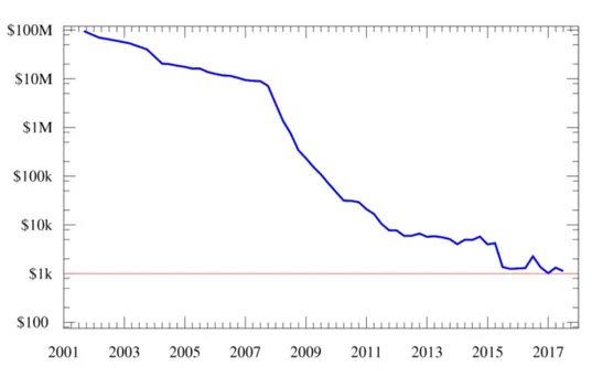
are now typically sequenced using new methods that have been developed over the past two decades. These methods, called Next Generation Sequencing (NGS) or High Throughput Sequencing (HTS), have significantly reduced the cost and ac-celerated the speed of large-scale sequencing. Figure 2.2 shows the Carlson curve, the biotechnological equivalent of Moore’s law, describing the rate of DNA se-quencing or cost per sequenced base as a function of time. Carlson predicted that the doubling time of DNA sequencing technologies (measured by cost and per-formance) would be at least as fast as Moore’s law. Actually, Moore’s Law started being profoundly out-paced in 2008, when sequencing centers transitioned to HTS technologies. This allowed researchers to achieve the “1000$ genome” goal
2.1. Genome sequencing 9
Figure 2.2: Carlson curve: total cost of sequencing a human genome over time
in 2017, and to set more ambitious objectives for the next years, like the “100$ genome” goal set by Illumina CEO [22].
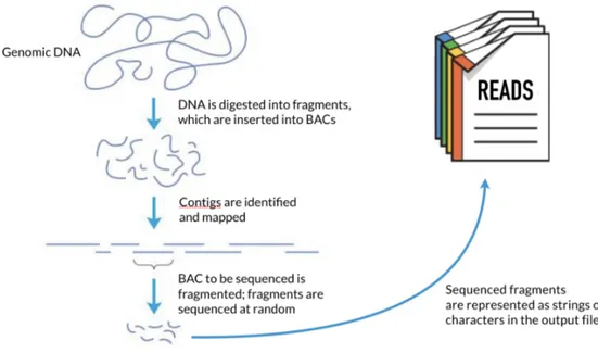
NGS technologies are typically characterized by being highly scalable, allow-ing the entire genome to be sequenced at once. Usually, this is accomplished by a process called shotgun sequencing, which consists of fragmenting the genome into small pieces, randomly sampling for a fragment, and sequencing it using one of a variety of available technologies. Multiple fragments are sequenced at once in an automated process, concurrently producing thousands or millions of text se-quences, called reads. Figure 2.3 gives an overview of the shotgun sequencing process.
As stated before, different new sequencing technologies have been developed in the last years, intended to lower the cost and the time of DNA sequencing [23].
Figure 2.3: Shotgun sequencing overview
These methods can be divided into three main categories, based on the length of the reads they produce, expressed in base pairs (bp):
• short read: ranging from 35 to 700 bp;
• long read: up to 80.000, with an average of 30.000 bp;
• ultra-long read: up to 1.000.000 bp, average depending on the experiment.
Short read technologies, led by Illumina platforms [24], are usually charac-terized by the highest throughput and scalability, and the lowest error rate (0,1%) and per sample cost [25]. Moreover, in addition to “classical” single-end reads, obtained by reading the DNA fragment only from one of its ends, many of these technologies can also produce paired-end and mate pair reads. In particular, in paired-end reading when the sequencer finishes one direction at the speci-fied read length, it starts another round from the opposite end of the fragment.
2.2. Genome assembly 11
Knowing the distance between each paired read helps to improve their specificity and effectively resolve structural rearrangements, as insertions and deletions. Al-though mate pair sequencing involves a much more complex process, the result is similar: a pair of reads separated by a known distance. The difference between the two variants is the length of the insert: 200-800 bp for paired-end, 2-5 kbp for mate pair reads.
Long read technologies, in particular Pacific BioSciences platforms [26], are able to produce reads at the highest speed, thus providing a good throughput. Long reads are useful to resolve structural rearrangements and repetitive regions, but their error rate on a single pass is still high (13%). The accuracy can be im-proved, reducing the error rate to 0,001%, with about 20 passes, but this approach significantly enlarges the cost and the time required for the experiments [25].
Finally, Oxford Nanopore Technologies platforms [27] can sequence ultra-long reads with, in principle, no upper limit to read length. They are characterized by good scalability, from extremely small and portable to extremely powerful and high throughput. However, their error rate is the highest (15%) and they suffer from systematic errors with homopolymers. Improved accuracy can be achieved (3% error rate) by reducing the throughput, at the cost of lower efficiency [25].
2.2
Genome assembly
The simplicity of the shotgun sequencing process captured the interest of mathe-maticians and computer scientists and led to the rapid development of the theo-retical foundations for genome sequence assembly. Because of the randomness of the fragmentation process, the individual fragments could be expected to
over-lap one another, and these overover-laps could be recognized by comparing the DNA sequences of the corresponding fragments. Scientists initially studied the com-putational complexity of the assembly problem formalized as an instance of the shortest common superstring problem, the problem of finding the shortest string that encompasses all the reads as substrings [28]. However, the shortest common superstring problem ignores an important feature of complex genomes: repeats. Most genomes contain DNA segments that are repeated in nearly identical form, thus the correct reconstruction of a genome sequence may not be the shortest. The need to explicitly account for repeats has led to new models of sequence as-sembly, but with such formulations, genome assembly can be shown to be com-putationally intractable [29]. Anyway, these negative theoretical results seem to be disconnected to the obvious practical success in sequence assembly witnessed over the past few decades. An explanation for this gap between theory and prac-tice is that theoretical intractability results are based on worst-case scenarios, which rarely occur in practice [30]. For this reason, in the last years practical assemblers were able to produce approximate, still very accurate, genome assem-blies, using different approaches that fall into several broad paradigms, outlined below.
2.2.1
De novo genome assembly
De novo genome assembly is very similar to solving a jigsaw puzzle, but without knowing the complete picture we are attempting to reconstruct. Rather all we have are the individual pieces (i.e. sequence reads) and the only way to build the final product is by understanding how each piece connects to another. Thus, de
2.2. Genome assembly 13
novo assembly constitutes a very complicated problem and, over the last decades, many approaches have been developed to resolve it.
The greedy approach works by making the locally optimal choice at each stage, hoping to find the global optimum. It starts by taking an unassembled read and then extends it by using the current read’s best overlapping read on its 3’ end. If the contiguous sequence, called contig, cannot be extended further, the process is repeated at the 5’ end of the reverse complement of the contig. Despite its simplicity, this approach and its variants provide a good approximation for the optimal assembly of small genomes, and many early genome assemblers relied on such a greedy strategy [31]. Anyway, greedy assemblers tend to misassemble big genomes by collapsing repeats and, as the size and complexity of the genomes being sequenced increased, they were replaced by more complex algorithms [32]. The Overlap-Layout-Consensus (OLC) approach, as the name suggests, con-sists of three steps. In the first one, an overlap graph is created by joining each read to its respective best overlapping one, similarly to the greedy approach. The layout stage, ideally, is responsible for finding one single path from the start of the genome traversing through all the reads exactly once and reaching the end of the sequenced genome. Anyway, this ideal scenario is usually not achievable and is the reason why we have so many algorithms trying to find the solution using the same scheme, but different heuristics. Finally, in the consensus stage, groups of reads that overlapped are evaluated in order to identify, by majority voting, which base should be present at each location of the reconstructed genome [29]. Despite this approach to assembly has been very successful, it struggles when pre-sented with the vast amounts of short-read data generated by NGS instruments. In practice, the overlap computation step is both a time and a memory
bottle-neck, as the memory requirements of these OLC assemblers grow quadratically with the depth of coverage and repeat copy number [30].
Graph-based sequence assembly models were developed to efficiently manage a vast amount of data, and they are the state of the art for the de novo genome as-sembly with high-throughput short-read sequence data. One of the most widespread methods is based on the de Bruijn graph, which has its roots in theoretical work from the late 1980s [33]. This approach consists in breaking each read into a sequence of overlapping k-mers, very short sequences of length k. The distinct k-mers are then used as vertices in the graph assembly, and k-mers that overlap by k−1 positions (e.g. originated from adjacent positions in a read) are linked by an edge. The assembly problem can then be formulated as finding a walk through the graph that visits each edge in the graph once: an Eulerian path problem [34]. In practice, sequencing errors and lack of coverage make it impossible to find a complete Eulerian tour through the entire graph, thus the assemblers attempt to construct contigs consisting of unambiguous, unbranching regions of the graph. The diffusion of de Bruijn graph approach is partially due to its significant computational advantage with respect to overlap-based assembly strategies: it does not require expensive procedures to identify overlaps between pairs of reads. Instead, the overlap between reads is implicit in the structure of the graph [30]. Moreover, a distinct advantage of de Bruijn graphs over traditional OLC meth-ods lies in the way the redundancy of high coverage NGS data is handled and ex-ploited. As each node must be unique, multiple overlaps between different reads just increase the count (frequency) of each k-mer contained in these overlaps, but not the number of nodes in the graph. As a result, de Bruijn graphs scale with the size and complexity of the target genome rather than the amount and length of the
2.2. Genome assembly 15
input reads. The main problem of this approach is that sequencing errors drasti-cally increase the complexity of de Bruijn graphs by introducing additional “fake” k-mers and therefore spurious branches [35]. Moreover, valuable context infor-mation stored within the reads is lost for assembly, because the k-mers have to be shorter than the actual read length. As a result, theoretically possible connections between different k-mers, which are not found in the original reads, artificially increase the complexity of the graph [32].
For the above-mentioned reasons, overlap based assembly methods have been revised, by integrating key elements of the de Bruijn graph, resulting in the string graph approach [36]. In particular, the de Bruijn graph has the elegant property that repeats get collapsed: all copies of a repeat are represented as a single seg-ment in the graph with multiple entry and exit points, providing a concise rep-resentation of the structure of the genome. A similar property can be obtained for overlap-based assembly methods by performing three operations. First, reads that are substrings of some other read are removed. Second, a graph is built where each sequence read is a vertex in the graph, and a pair of vertices are linked with an edge if they overlap. Third, transitive edges are removed from the graph. The result is a drastically simplified and directed overlap graph, called string graph, with basically the same properties and advantages as a de Bruijn graph, but more sequence information represented by every node and edge. However, a major disadvantage of overlap-based approaches remains, since the search for overlaps still requires alignments between every possible read combination. This makes all overlap based approaches, string graph as well as OLC, extremely time-consuming for large sequencing datasets. Anyway, assemblers utilizing the string graph method are definitively not out of the picture and they are even
experienc-ing a renaissance with the increase in read lengths of NGS technologies [37].
2.2.2
Comparative genome assembly
With the rapid growth in the number of sequenced genomes has come an increase in the number of organisms for which two or more closely related species have been sequenced. This led to the possibility of creating comparative genome as-sembly algorithms, which can assemble a newly sequenced genome by mapping it onto a similar reference genome [38].
Looking back at the analogy with the jigsaw puzzle, in comparative assem-bly we have access to the complete or partial picture of the final product, but some of our puzzle pieces are distorted or torn apart. Even though there is not a complete correspondence between the newly sequenced genome and the refer-ence one, having a “backbone” sequrefer-ence significantly easies the task of putting the pieces together in the right place. In fact, in order to properly order the mas-sive number of reads sequenced by NGS instruments, we don’t need anymore to compute the expensive pairwise alignments of all the reads against each other, as in overlap-based de novo aligners.
Instead, comparative assemblers usually rely on the alignment-layout-consensus paradigm [32]. In the alignment stage, reads are mapped to the reference genome, admitting multiple alignments of the same read to different genome’s location, and resolving some of these ambiguities by using paired-end or mate pair reads. The alignment of all the reads produce a layout but, because we are aligning reads derived from an unknown target genome to a related reference genome that is slightly different, many reads might not align perfectly due to some mismatches,
2.3. Genomic analysis 17
insertions, deletions or structural variations. These issues are faced by iteratively refining the layout, resolving the divergent areas by generating a consensus se-quence and then using that as a template for the alignment. This step is repeated until the issues identified above are not faced anymore.
Even if knowing the reference sequence remarkably reduce the complexity of the genome assembly problem, the alignment of a massive number of reads against a long reference sequence still constitutes a time bottleneck in the assem-bly process. For this reason, many aligners developed in the last decades rely on the seed and extend paradigm [39], consisting of two steps. First, short sequences called seeds are extracted from the reads set and are mapped onto the reference genome by looking for exact matches between the seeds and the reference se-quence. Then, regions of the reference containing a high number of seeds from the same read are selected as candidates for the extension phase, that consists of aligning the reads to their candidate regions through a dynamic programming al-gorithm. This approach minimizes the search space, avoiding the need for com-puting several expensive alignments against the long backbone sequence, thus appreciably lowering the complexity of the assembly process.
2.3
Genomic analysis
The DNA sequence assembly alone is not very significant per se, as it requires additional analysis. Once a genome is sequenced and assembled, it needs to be annotated to make sense of it. Genome annotation is defined as the process of identifying the locations of genes and all of the coding regions in a genome and determining what those genes do [40]. The biological information is then
at-tached to the respective sequence element, in the form of an explanatory or com-mentary note. Thus, identified genes are referred to as annotated.
The genome annotation process consists of three steps:
1. identifying non-coding regions of the genome;
2. identifying coding elements on the genome, through a process called gene prediction;
3. attaching biological information to the identified elements;
Usually, automatic computer analysis and manual annotation involving human expertise co-exist and complement each other in the same annotation pipeline.
The first two steps of the annotation process are generally referred to as struc-tural annotation. This part of the genomic analysis consists of identifying all and only the genomic elements of interest, like genes, regulatory motifs, and open reading frames. Information about their localization and structure are added to the assembled genome during this phase. The last step instead, namely func-tional annotation, consists of attaching to the identified elements information about their biochemical and biological function, expression, and involved reg-ulation and interactions [41]. The most employed approach for gene annotation relies on homology-based search tools to look for homologous genes in specific databases; the resulting information is then used to annotate genes and genome. In practice, this means that a variety of known sequences are mapped onto the as-sembled genome, in order to identify some of its coding regions and understand their function.
2.3. Genomic analysis 19
Another important piece of the genomic analysis is variant calling, which is the identification and analysis of variants associated with a specific trait or pop-ulation [42]. Genetic variations are the differences in DNA sequences between individuals within a population, and they can be caused by mutations, that are permanent alterations to the sequence due to errors during DNA replication, or by recombination, that is the mixing of parental genetic material which occurs when homologous DNA strands align and cross over. There are three main types of genetic variation:
• Single Nucleotide Polymorphism (SNP): substitution of a single base-pair;
• Indels: insertion or deletion of a single stretch of DNA sequence ranging from one to hundreds of base-pairs in length;
• Structural Variation: genetic variations occurring over a larger DNA se-quence, as copy number variation or chromosomal rearrangement events.
These genetic differences between individuals are crucial not only because they lead to differences in an individual’s phenotype, but also because they are related to the risk of developing a particular disease, due to their effects on protein struc-tures [43]. Again, the variant calling process involves the expensive alignment of sequencing data to a reference genome, in order to identify where the aligned reads differ from it and classify these differences.
As introduced in Chapter 1, genome sequencing, assembly and analysis are the core of precision medicine, which takes into account individual variability in genes in order to find the best treatment for a particular disease, in a certain group of individuals. This approach has the potential for improving many aspects
of health and healthcare, and can provide a better understanding of the under-lying mechanisms by which various diseases occur. For example, identifying the cancer-causing genes allows researchers to study drugs that target those genes, in order to deactivate them and attack the cancer cells. It is clear that, in an era where genome sequencing is becoming faster and cheaper, the main threat to the development and spreading of precision medicine is given by the long time and the high cost required by genome assembly and genomic analysis. In particular, sequence alignment constitutes the space and time bottleneck for most of the ex-isting approaches to both these problems, and researchers are constantly looking for solutions that can lower the complexity of this task.
Because of the aforementioned reason, this thesis will present a space-efficient short read mapper, that can find application in de novo and comparative genome assembly, as well as in genome annotation or variant calling pipelines. Its user-friendly web-based interface and the support for standard file formats respectively guarantees high usability and easy integration in most of the existing bioinfor-matic pipelines. Moreover, the proposed tool leverages the FPGA architecture in order to obtain the best performance over power ratio, trying to match the needs of pharmaceutical industries and those of the researchers’ community, in the aim of contributing to the spreading and to the democratization of precision medicine.
CHAPTER
3
Problem Description
T
o allow the reader a better understanding of the works analyzed in the literature, within this Chapter the Burrows-Wheeler Map-ping problem and the methods employed in this work are pre-sented. Section 3.1 gives a description of the standard file for-mats used to store genomic sequences, while Section 3.2 describes the Burrows-Wheeler Transform, the FM-Index, and the backward search algorithm. Then, Section 3.3 introduces the concept of Succinct Data Structure, focusing on the two structures employed in this implementation: RRR and wavelet trees. Finally, Section 3.4 gives an overview of the available hardware accelerators and a descrip-tion of the FPGA architecture.3.1
Genomic sequences: FASTA and FASTQ file format
As stated in Section 2.1, sequencing technologies digitalize the information con-tained in DNA fragments, encoding it in text sequences called reads. In the field
of bioinformatics, the universal standard is FASTA format, a text-based format for representing either nucleotide sequences (DNA or RNA) or amino acid se-quences (protein) [44]. The format allows for sequence names and comments to precede the sequences, where nucleotides and amino acids are represented us-ing sus-ingle-letter codes. The header/identifier line, which begins with a ‘>’, gives a name and/or a unique identifier for the sequence, and may also contain addi-tional information, like Naaddi-tional Centre for Biotechnology Information (NCBI) identifiers.
FASTQ format is an extension of FASTA format, for storing a nucleotide se-quence and its corresponding quality scores, where both the sese-quence letter and quality score are encoded with a single ASCII character [45]. Originally devel-oped at the Wellcome Trust Sanger Institute to bundle a FASTA formatted se-quence and its quality data, it has recently become the de facto standard for stor-ing the output of high-throughput sequencstor-ing instruments. A FASTQ file uses four lines per sequence:
1. header line: begins with a ‘@’ character and is the equivalent of FASTA identifier line
2. sequence line: contains the raw sequence letters
3. separation line: begins with a ‘+’ character and is optionally followed by the same information contained in the header line
4. quality line: encodes the quality values for the sequence letters in line 2, and must contain the same number of symbols as letters in the sequence
3.2. Burrows-Wheeler Mapping 23
Quality values Qi are integer mappings of pi, that are the probabilities that the
corresponding base calls are incorrect. The equation for calculating Qiis the
stan-dard Sanger equation to assess the reliability of a base call, otherwise known as Phred quality score:
Qi =−10 log10(pi). (3.1)
3.2
Burrows-Wheeler Mapping
Finding a match between a query sequence and a long reference with a naive ap-proach is a computationally intensive task, requiring to scan the whole reference sequence while looking for a certain pattern. For this reason, many approaches to resolve this task are based on indexing strategies, that allow to reduce the search space and speed up the matching process. Among these approaches, Burrows-Wheeler Mapping is well known because of its trivial time complexity. In prac-tice, it consists of performing a backward pattern matching against a reference in a time that only depends on the pattern length, but not on the reference length. The backward pattern matching algorithm is presented in the remainder of this Section, together with the three concepts it is based on: suffix arrays, Burrows-Wheeler Transform, and FM-index.
LetT [1, N] be a sequence of length N drawn from a constant-size alphabet ∑
, and letT [i, j] denote the substring of T ranging from i to j. The Suffix Array SA built on T is an array containing the lexicographically ordered sequence of the suffixes ofT , represented as integers providing their starting positions in the sequence. This means that an entrySA[i] contains the starting position of the
i-th smallest suffix inT , and thus
∀ 1 < i ≤ N : T [SA[i − 1], N] < T [SA[i], N] . (3.2)
It follows that if a stringX is a substring of T , the position of each occurrence ofX in T will occur in an interval in the suffix array. This is because all the suffixes that haveX as prefix are sorted together. Based on this observation, we define:
start(X ) = min{i : X is the prefix of T [SA[i], N]} (3.3)
end(X ) = max{i : X is the prefix of T [SA[i], N]} . (3.4)
The interval [start(X ), end(X )] is called the suffix array interval of X , and the positions of all the occurrences ofX in T are contained in the set
{SA[i] : start(X ) ≤ i ≤ end(X )}.
Thus, pattern matching is equivalent to searching for the SA interval of sub-strings ofT that match the query.
The suffix array of a string is closely related to its Burrows-Wheeler Trans-form (BWT), which is a reversible permutation of the characters in the string [46]. This transformation was originally developed within the context of data compression because it rearranges a text into runs of similar characters, making it easily compressible. However, since BWT-based indexing allows large text to be searched efficiently, it has been successfully applied to bioinformatic applica-tions, such as oligomer counting [47] and sequence alignment [11, 48, 49]. The
3.2. Burrows-Wheeler Mapping 25
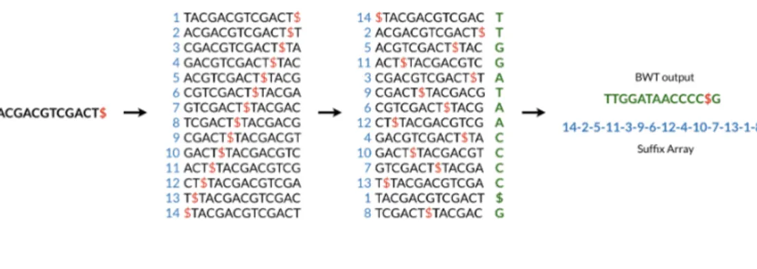
Figure 3.1: Burrows-Wheeler Transform and Suffix Array construction
Burrows-Wheeler Transform of a sequenceT , BW T (T ), can be constructed as follows:
1. the character $ is appended toT , where $ is not in the alphabet∑and it is considered lexicographically smaller than all symbols in∑;
2. the Burrows-Wheeler matrix ofT is constructed as the [(N +1)∗(N +1)] matrix whose rows contain all cyclic rotations ofT $;
3. the rows are sorted into lexicographical order;
4. BW T (T ) is the sequence of characters in the rightmost column of the Burrows-Wheeler matrix.
Figure 3.1 gives a graphical representation of the BW T (T ) construction, and it shows how it is possible to compute the suffix array ofT at the same time.
The Burrows-Wheeler matrix has a very important property called last-first mapping: the i-th occurrence of character c in the last column corresponds to the same text character of the i-th occurrence of c in the first column. This feature underlies algorithms that use BWT-based indexes to navigate or search the text,
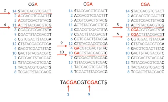
Figure 3.2: The backward pattern matching procedure
like the backward pattern matching algorithm employed in this work. Since the matrix is sorted in lexicographical order, rows beginning with a given sequence appear consecutively. The backward search procedure, showed in Figure 3.2, it-eratively calculates the range of matrix rows beginning with longer suffixes of the query. At each step, the size of the interval either shrinks or remains the same. When the execution stops, rows beginning with the entire query sequence corre-spond to occurrences of the query in the text, and their positions can be found in the correspondent range of the suffix array.
Ferragina and Manzini, to whom the backward pattern matching algorithm can be attributed, presented two data structures that allow to rapidly execute the search:
• the array C stores, for each symbol in∑, the number of characters with a lower lexicographical value; thus, C(x) is the number of symbols in BW T (T )
3.3. Succinct Data Structures 27
that are lexicographically smaller than x,∀x ∈∑;
• the matrix Occ stores the number of occurrences of each symbol up to a certain position in BW T (T ); thus Occ(x, i) is the number of occurrences of x in BW T (T )[1, i].
The authors proved that ifX is a substring of T :
start(aX ) = C(a) + Occ(a, start(X ) − 1) + 1 (3.5)
end(aX ) = C(a) + Occ(a, end(X )) (3.6)
and that start(aX ) ≤ end(aX ) if and only if aX is a substring of T . This result makes it possible to count the occurrences ofX in T in O(|X |) time, by iteratively calculating start and end from the end ofX , as showed in Algorithm 1.
3.3
Succinct Data Structures
Every living thing on Earth, from humans to bacteria, has a genome. The size of a genome varies a lot from species to species and it seems to be only slightly related to the complexity of the organism it belongs. For instance, the genome of Viroids (smallest known pathogens) is only∼ 300 nucleotides long, while the human genome has a length of more than 3.2 billions bp. Anyway, our genome is not the biggest one; actually, it looks quite small if compared to that of Amoeba Dubia, a very tiny creature, whose genome is∼ 670 billions bp long, making it the biggest known genome. This means that, assuming to encode each nucleotide in a byte, we would need 670 GB of memory just to store the sequence. Given this
Input: The query pattern P [1, p]
Output: Number of occurrences of P [1, p] begin i = p; c = P [p]; start = C[c] + 1; end = C[c + 1]; end
while ((start≤ end) and (i ≥ 2)) do
c = P [i− 1];
start = C[c] + Occ[c][start− 1] + 1; end = C[c] + Occ[c][end];
i = i− 1;
end
if start≤ end then
return “found (end− start + 1) occurrences” end
else
return “pattern not found” end
Algorithm 1: Backward search algorithm
knowledge, it turns out that storing this enormous amount of data in a compact space, and making it easily accessible, is a challenging but crucial requirement for enabling some bioinformatic applications. Here is where succinct data structures come into play.
Succinct data structures are defined as data structures which use an amount of space close to the information-theoretic lower bound, but still allow for efficient query operations. Unlike general lossless compressed representations, succinct data structures have the unique ability to use data in-place, without decompress-ing them first. A succinct data structure, encoddecompress-ing a sequenceT [1, N], has to allow three operations on the data:
3.3. Succinct Data Structures 29
Figure 3.3: Wavelet tree of the sequence TTGGATAACCCC$G
2. rankC(T , i): returns the number of occurrences of character C in T [1, i];
3. selectC(T , i): returns the position of the i-th character C in T , with 1 ≤
i≤ rankC(T , N).
In this work, a combination of two different data structures is employed to encode the reference sequence in an efficient way: wavelet trees and RRR sequences.
3.3.1
Wavelet Tree
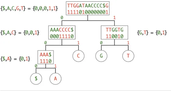
A wavelet tree is a succinct data structure to store a stringT [1, N], from an alpha-bet∑, in a compressed space of N log2(|∑|) bits. Wavelet trees convert a string into a balanced binary tree of bit-vectors, where a 0 replaces half the symbols of the alphabet, and a 1 replaces the other half. At each level, the alphabet is filtered and re-encoded, in order to reduce the ambiguity, until there is no ambiguity at all. The tree is defined recursively as follow:
1. encode the first half of the alphabet as 0, the second half as 1 (e.g. {A,C,G,T} would become {0,0,1,1});
2. group each 0-encoded symbol (e.g. {A,C}) as a sub-tree;
3. group each 1-encoded symbol (e.g. {G,T}) as a sub-tree;
4. recursively apply this steps to each sub-tree until there are only 1 or 2 sym-bols left (no more ambiguity, a 0 or a 1 can only encode one symbol).
Figure 3.3 shows the wavelet tree of the sequenceT = TTGGATAACCCC$G. Please note that the sequences are only showed for the seek of clarity, while in the actual implementation only bit-vectors are stored in the nodes of the wavelet tree. After the tree is constructed, a rank query can be done with log2(|∑|) binary rank queries on the bit-vectors. For example, if we want to know rankA(T , 11),
we use the following procedure. Knowing that A is encoded as 0 at the first level, we calculate the binary rank query of 0 at position 11, which is 6. Then we use this value to indicate where to calculate the binary rank of the 0-child. This procedure is applied recursively until a leaf node is reached, as illustrated in Figure 3.4.
3.3.2
RRR Data Structure
The RRR theoretical data structure is named after its creators: Raman, Raman, and Rao [50]. The purpose of RRR is to encode a bit sequenceB[1, N] in such a way that supports O(1) time binary rank queries. Moreover, it provides implicit compression, requiring N H0(B)+o(N), where H0(B) is the zero-order empirical
3.3. Succinct Data Structures 31
Figure 3.4: A rank query on the wavelet tree
be calculated as H0(X ) = σ ∑ i=1 Ni N log( N Ni ) (3.7)
where Ni is the number of occurrences of the i-th element of
∑
in the sequence X . The RRR structure can be constructed as follow:
1. divide the bit-vectorB into blocks of b bits each;
2. group these blocks in superblocks of sf × b bits and, for each superblock, store the sum of previous ranks1(B) at the superblock boundary;
3. for each block, store a class number c, that is the number of 1s in the block;
4. build a table P , which has subtables P [c] for each class c. For each permu-tation ci of c 1s over a b-bits block, P [ci]contains an array of cumulative
5. for each block, store an offset off which is an index into the table P pointing to the permutation corresponding to the considered block.
The resulting data structure can answer rank1(B, i) query in constant time,
ac-cording to the following procedure:
1. calculate which block the index is in as ib = ib;
2. calculate which superblock the index resides in as is = sfib;
3. set the temporary result to the sum of previous ranks at isboundary;
4. add to the result the rank of entire blocks (their classes) after is, until ib is
reached;
5. finally, add P [off(ib)][j], where j = i mod b.
The final result is the answer to the initial rank1(B, i) query.
3.4
Hardware Accelerators
Bioinformatic applications usually require to execute computationally intensive algorithms on a vast amount of data. Indeed, a software implementation on a gen-eral purpose Central Processing Unit (CPU) is the fastest to realize, because this platform offers good flexibility and an easy design process. Anyway, such a choice could be inefficient from an energetic and execution time perspective. Following the needs of pharmaceutical industries and those of the researchers’ community, moving the implementation to hardware is the best way to optimize bioinformatic algorithms. In this context, there are different platforms upon which the user can choose to implement the algorithm, such as Application Specific Integrated
3.4. Hardware Accelerators 33
Circuits (ASICs), Graphical Processing Units (GPUs) and Field Programmable Gate Arrays (FPGAs). ASICs are the best solution both from a performance and power consumption point of view. However, the design and development cost of an ASIC is very high and only justified in case of a large number of deployed sys-tems. In addition, these systems are not reconfigurable, so not flexible. It follows that, once the chosen algorithm is implemented, no changes can be made to the design. Reconfigurability is a feature of both GPUs and FPGAs, so both of them are pretty flexible solutions. GPUs, thanks to their architecture, can consider-ably accelerate certain types of algorithms, although their power consumption is substantially high. FPGAs, instead, offer a good trade-off between performance and power consumption. Thanks to their flexibility and lack of a fixed hardware architecture, FPGAs can be configured and reconfigured by the user to imple-ment different functions. A hardware impleimple-mentation on FPGA would give the benefit of a speedup over a pure software implementation while reducing power consumption. Moreover, the development cost of an application to run on an FPGA is remarkably lower compared to the ASIC one.
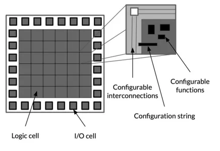
At the highest level, FPGAs are reprogrammable silicon chips. An FPGA is an array of logic blocks (cells) placed in an infrastructure of interconnections, which can be programmed at three distinct levels: the function of the logic cells, the interconnections between cells, and the inputs and outputs (Figure 3.5). All three levels are configured via a string of bits that is loaded from an external source. Any logic block (Figure 3.6) contains a Look-Up Table (LUT), a register and a multiplexer (MUX), and it can perform different functions, depending on how the Static Random Access Memory (SRAM) is programmed. The content of the SRAMs cells determines the content of the LUTs and, subsequently, the logic
Figure 3.5: FPGA overview
3.4. Hardware Accelerators 35
function realized. The registers act as flip-flops in sampling, and the inputs they receive are selected by the multiplexers.
Modern FPGA families expand upon the above capabilities to include higher level functionality fixed into the silicon. Having these common functions embed-ded into the silicon reduces the area required and gives those functions increased speed compared to building them from primitives. Examples of these include multipliers, generic Digital Signal Processor (DSP) blocks, embedded processors, high speed I/O logic and embedded memories. These components integrated into the FPGAs aren’t reprogrammable (except the connections to which they are connected) and perform specific functions, allowing to lighten the weight of the logic functions that the reprogrammable logic blocks have to implement.
Although the possible advantages of using such an architecture are clear, de-signing on an FPGA is a complicated procedure, as the design process is dif-ferent from regular software development. Fortunately, in the last years, many toolchains have been created, aiming to facilitate this procedure. Among these, the SDAccel toolchain by Xilinx [51] is a complete design environment, provid-ing raised abstraction for accelerators, simplified host integration and automated infrastructure creation. Users are supported during the whole hardware design flow: High-Level Synthesis (HLS) eases the creation and optimization of the hard-ware cores, and a guided System-Level Design (SLD) allows their implementation on the targeted board.
For the aforementioned reasons, the FPGA seems to be the best target for the proposed application. In fact, by leveraging its reconfigurability capabilities is possible to create a hardware implementation aiming at power over performance ratio optimization, in accordance with the needs of the bioinformatic community.
CHAPTER
4
Related work
T
his Chapter presents a review of the State of the Art for the em-ployed methodologies. Section 4.1 explains the different approaches found in literature for the read alignment against large references, with particular emphasis on the Burrows-Wheeler Mapping. Sec-tion 4.2 will describe the details of the best performing hardware implementa-tions of the Burrows-Wheeler based alignment, while Section 4.3 will present the difficulties bioinformaticians have to face because of the low usability of open source tools.4.1
Read alignment and Burrows-Wheeler mapping
As introduced in Chapter 2, read alignment is the computational bottleneck of several bioinformatic applications, such as de novo and comparative genome as-sembly, variant calling and genome annotation. For this reason, in the last years, researchers put a big effort into the development of different approaches and
4.1. Read alignment and Burrows-Wheeler mapping 37
gorithms that could lower the complexity of this task. The vast majority of se-quence aligners relies on Dynamic Programming (DP), an optimization method consisting in storing the results of sub-problems so that it is not necessary to re-compute them when needed later. Dynamic Programming can be used to address the sequence alignment problem in all its formulations (i.e. global, local, glocal). Global alignment algorithms find the optimal end-to-end alignment of two se-quences, thus they are particularly useful when comparing two similar sequences that have almost the same length. Needleman-Wunsch algorithm [7] was one of the first applications of dynamic programming to compare biological sequences, and after almost 50 years since its publication, it is still the core of many global alignment tools used today [52]. Moreover, little modifications to Needleman-Wunsch algorithm make it suitable for finding the glocal alignment between two sequences, that is the best possible partial alignment where gaps at the beginning and/or at the end of one sequence (or even both) are ignored. This is particularly useful when the final part of one sequence overlaps with the beginning part of the other one, or when one sequence is much shorter than the other one [9]. Fi-nally, local alignment algorithms search for optimal alignment between local por-tions of the given sequences, thus they are useful for dissimilar sequences that are suspected to contain a region of similarity within their larger sequence context. Smith-Waterman algorithm [8], which is also based on dynamic programming, is the most employed local alignment algorithm in the literature [52, 53].
Regardless of the chosen sequence alignment formulation, DP-based approaches search for the optimal alignment and have quadratic time complexity w.r.t the length of the aligned sequences [54]. Thus, employing these techniques alone of-ten leads to prohibitive execution times, especially when the number of sequences
to be aligned is very high (e.g. overlap-based de novo genome assembly), or when sequences are very long (e.g. comparative genome assembly). For this reason, many aligners developed in the last years have coupled DP-based alignment al-gorithms with heuristics which allow to reduce the search space and speed up the alignment process. The most employed heuristic approach is called seed and ex-tend, and it proved to achieve an excellent tradeoff between speed and accuracy [39]. This technique consists of two steps:
1. seeding is finding exact matches of parts of the query sequence with parts of the reference;
2. extending is executing a DP-based alignment algorithm in a local neigh-borhood of the regions identified in the seeding process.
Modern aligners use two kind of seeds: fixed-length seeds [12, 18, 55], and max-imal exact matching (MEM) seeds [11, 56]. Fixed-length seeds, as the name sug-gests, are simply overlapping or non-overlapping substrings of the reads, all hav-ing the same length. MEM seeds, instead, are the longest matches which cannot be further enlarged in either direction [10].
In order to make seed and extend approach effective, the seeding step needs to be very fast, thus it usually requires a pre-built index of the reference genome. The majority of contemporary sequence aligners compute seeds by either using hash table indices [18, 55] or using BWT-based indices, such as the FM-index [11, 12, 57]. The latter offer an important advantage over the former: their memory usage is independent of the number of reads to be aligned, instead of growing linearly with it. The most relevant and widespread BWT-based aligners are the
4.1. Read alignment and Burrows-Wheeler mapping 39
Burrows-Wheeler Aligners (BWA [48], BWA-SW [58] and BWA-MEM [11]) and the two versions of Bowtie [49, 12].
BWA [48] and Bowtie [49] use modified versions of the backward search al-gorithm presented in Section 3.2 to calculate also inexact matches of the query with the reference, and even gapped alignments in the case of BWA. However, the time complexity of these strategies grows exponentially with the number of mismatches, thus these tools allow only few differences between sampled short substrings of the reference and entire query sequences [39]. In order to improve speed, fraction of reads aligned, and quality of the alignments, next versions of the aforementioned tools adopted a seed and extend strategy, coupling the FM-index with DP-based alignment algorithms. In particular, Bowtie2 [12] extracts fixed-length seeds and maps them onto the reference sequence through the same backward search process used in Bowtie, allowing up to a mismatch. Then it ap-plies a seed alignment prioritization, associating to each seed hit (i.e. a locus of the reference sequence that matches the seed) a score which is inversely propor-tional to the number of loci matched by that seed. Finally, each reference locus is passed, according to its priority, to a SIMD-accelerated DP-based alignment algorithm (global or local), along with information about which seed string gave rise to the hit. BWA-SW [58], instead, builds FM-indices for both the reference and query sequence, representing the reference sequence in a prefix trie and the query sequence in a prefix Directed Acyclic Word Graph (DAWG). The two data structures are then aligned through dynamic programming, employing a couple of heuristics to speed up the process. Although this strategy reduces the number of computational expensive alignments to be computed, it leads to larger memory usage. Moreover, BWA-SW generally shows longer execution time w.r.t. Bowtie2