Aquifer characterization at field scale under architecture and model uncertainty

Scuola di Ingegneria Civile, Ambientale e Territoriale

C

orso di Laurea Magistrale in Ingegneria Civile

Aquifer characterization at field scale under architecture

and model uncertainty

Relatore: Prof. Riva Monica

Correlatore: Dr. Bianchi Janetti Emanuela

Tesi di Laurea Magistrale di:

Gian Luca Grassi

Matr. 839020

I

INDEX

ABSTRACT – ENG

ABSTARCT – ITA

1. INTRODUCTION

1.1 THE “NATURAL SPINGS BELT” IN THE PADANA PLANE ……….………6

1.2 DEVELOPPING OF THE MODEL ……….………9

2. THEORETICAL BACKGROUND

2.1 GROUNDWATER FLOW MODEL ……….…….………….………….………….……….13

2.1.1 FINITE-DIFFERENCE EQUATION ……….………....14

2.1.2 RESOLUTION OF THE EQUATION ……….………..18

2.2 SENSITIVITY ANALYSIS ……….………….………….………….………...20 2.2.1 MORRIS …….………….………….………….………….………….………21 2.2.2 SOBOL …….………….………….………….………….………….………..22 2.3 PARAMETER ESTIMATION …….………….………….………….………….……….25 2.3.1 PEST ……….25 2.3.2 PEST ALGORITHM …….………….………….………….………….…………27 2.3.2.1 LINEAR MODEL ……….………….………….………. 28 2.3.2.2 NON-LINEAR MODEL …….………….………….………..30 2.3.3 PEST IN MODFLOW ..…….………….………….………….………..31

2.4 MODEL VALIDATION CRITERIA ……….………….………….………….……….32

3. CONCEPTUAL AND MATHEMATICAL MODEL

3.1 STUDY AREA …….………….………….………….……….35

3.2 CONCEPTUAL MODEL ………36

3.2.1 COMPOSITE MEDIUM MODEL ………..37

3.2.2 OVERLAPPING CONTINUA MODEL ……….38

3.3 MATHEMATICAL MODEL ………..39

3.3.1 MODEL DOMAIN ……….39

3.3.2 BOUNDARY CONDITIONS ……….40

3.3.2.1 URBAN ZONE ………..43

3.3.2.2 NON-URBAN ZONE ……….49

3.3.2.3 NORTH BOUNDARY CONDITION ………60

II

4.2 MORRIS INDICES ………..63

4.2.1 COMPOSITE MEDIUM ……….63

4.2.2 OVERLAPPING CONTINUA – ARITHMETIC AVERAGE ………….69

4.2.3 OVERLAPPING CONTINUA – GEOMETRIC AVERAGE ………….73

4.3 SOBOL INDICES ………..77

4.3.1 COMPOSITE MEDIUM ……….77

4.3.2 OVERLAPPING CONTINUA – ARITHMETIC AVERAGE ………….81

4.3.3 OVERLAPPING CONTINUA – GEOMETRIC AVERAGE ………….84

4.4 COMPARISON ……… 88

5. MODEL CALIBRATION

5.1 CALIBRATION OF MODEL PARAMETERS ….………...96

5.2 COMPOSITE MEDIUM ………..99

5.3 OVERLAPPING CONTINUA – ARITHMETIC AVERAGE ………109

5.4 OVERLAPPING CONTINUA – GEOMETRIC AVERAGE ……… 119

5.5 COMPARISON BETWEEN THE MODELS ……….129

6.

CONCLUSIONS

ANNEXES

-

BIBLIOGRAPHY

III

1.1 - Natural springs in the Lombardia region ………5

1.2 - Scheme of the Padana plane ………6

2.1 - Six adjacent cells around the cell I,j,k, McDonald and Harbaugh representation …………..………14

2.2 - Flow coming from cell I,j-1,k into cell I,j,k ……….15

3.1 - Localization of the Area of study ………35

3.2 – Variation of temperature in 2015 for the seven hydrological stations ………41

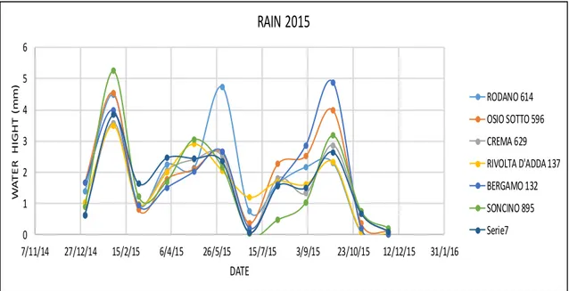
3.3 - Amount of rain fallen in the year 2015 for the seven considered meteorological stations ………..42

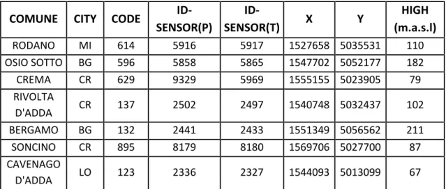
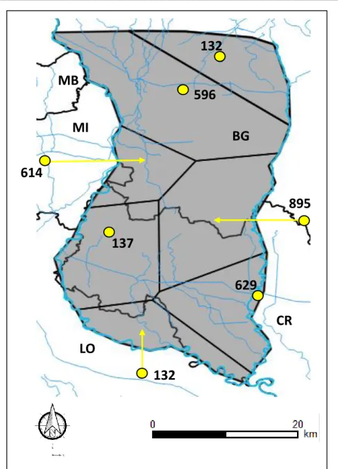
3.4 - Spatial distribution of the meteorological stations and Thiessen polygons used in the model ….………...43

3.5 - Urbanized Area in the Big Scale Model …….……….44

3.6 - Location of withdrawal wells ………..……….46

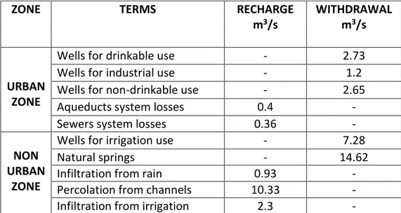
3.7 - Representation of the terms involved in the Urban Area for the hydrological balance …..………48

3.8 - Natural springs within the Cremona region ……….……….……….51

3.9 - Flow pumped out from each of the five more relevant channels within the area. The green line represents the total amount of water pumped, obtained by a summation from the contributions given by the five channels .………58

3.10 - Representation of the terms involved in the Non-Urban Area for the hydrological balance ….……….59

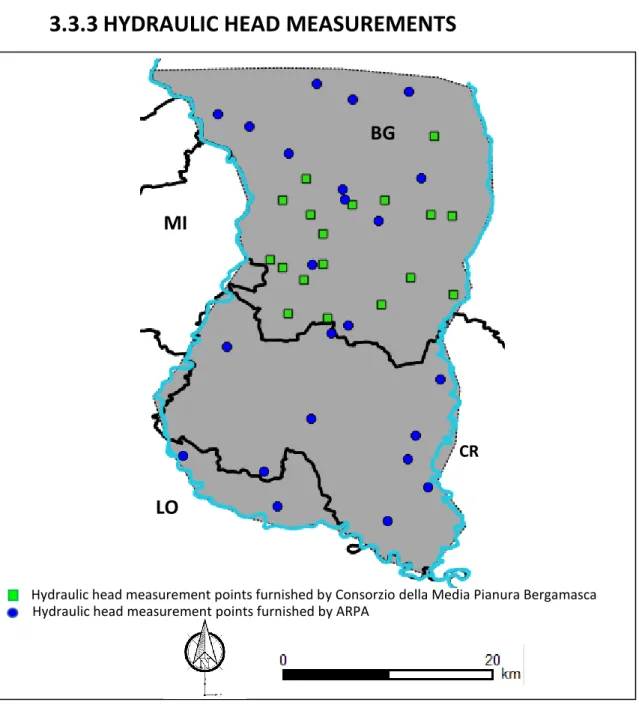
3.11 - Representation of the hydraulic head measurement points given by ARPA and by the Consorzio della media pianura bergamasca ……….60

4.1 – Distribution of μ* evaluated at the 40 hydraulic head measurements points for the Composite Medium case. The upper limit of the box represents the 75 percentiles of the distribution while the lower one is the 25 percentiles. The straight line inside the box is the median and the dots are the averages. Whiskers goes until the 95 percentiles the 5 percentiles, while the red crosses are the outliers of the distributions ……..64

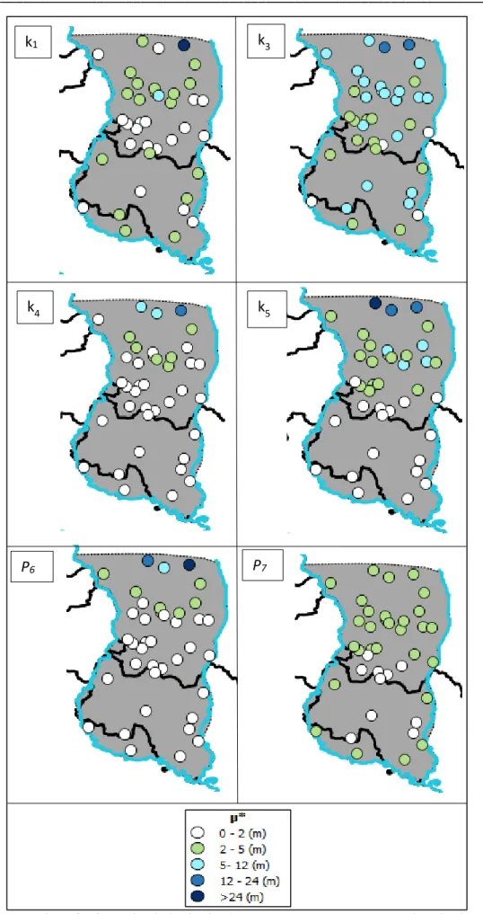
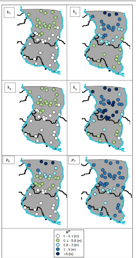
4.2 - Value of μ* in the hydraulic head measurements points associated with the variation of four parameters and two boundary conditions .………...66

4.3 – North and South zone of the model ……….………67 4.4 - Distribution of μ* evaluated at the 29 hydraulic head measurements points for the Composite Medium case in the northern zone. The upper limit of the box represents the 75 percentiles of the distribution while the lower one is the 25 percentiles. The straight line inside the box is the median and the dots are the average. Whiskers goes until the

IV

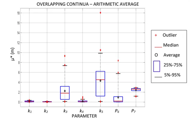
4.5 - Distribution of μ* evaluated at the 11 hydraulic head measurements points for the Composite Medium case in the southern zone. The upper limit of the box represents the 75 percentiles of the distribution while the lower one is the 25 percentiles. The straight line inside the box is the median and the dots are the average. Whiskers goes until the 95 percentiles the 5 percentiles, while the red crosses are the outliers of the distributions: ……….……….68 4.6 - Distribution of μ* evaluated at the 40 hydraulic head measurements points for the Overlapping Continua with arithmetic average case. The upper limit of the box represents the 75 percentiles of the distribution while the lower one is the 25 percentiles. The straight line inside the box is the median and the dots are the average. Whiskers goes until the 95 percentiles the 5 percentiles, while the red crosses are the outliers of the distributions: ………69 4.7 - Value of μ* in the hydraulic head measurements points associated with the variation of four parameters and two boundary conditions .………71 4.8 - Distribution of μ* evaluated at the 29 hydraulic head measurements points for the Overlapping Continua with arithmetic average case in the northern zone. The upper limit of the box represents the 75 percentiles of the distribution while the lower one is the 25 percentiles. The straight line inside the box is the median and the dots are the average. Whiskers goes until the 95 percentiles the 5 percentiles, while the red crosses are the outliers of the distributions: ……….………..72 4.9 - Distribution of μ* evaluated at the 11 hydraulic head measurements points for the Overlapping Continua with arithmetic average case in the southern zone. The upper limit of the box represents the 75 percentiles of the distribution while the lower one is the 25 percentiles. The straight line inside the box is the median and the dots are the average. Whiskers goes until the 95 percentiles the 5 percentiles, while the red crosses are the outliers of the distributions: ……….73 4.10 - Distribution of μ* evaluated at the 40 hydraulic head measurements points for the Overlapping Continua with geometric average case. The upper limit of the box represents the 75 percentiles of the distribution while the lower one is the 25 percentiles. The straight line inside the box is the median and the dots are the average. Whiskers goes until the 95 percentiles the 5 percentiles, while the red crosses are the outliers of the distributions ……….…….74 4.11 - Value of μ* in the hydraulic head measurements points associated with the variation of four parameters and two boundary conditions .……….75 4.12 - Distribution of μ* evaluated at the 29 hydraulic head measurements points for the Overlapping Continua with geometric average case in the northern zone. The upper limit of the box represents the 75 percentiles of the distribution while the lower one is the 25 percentiles. The straight line inside the box is the median and the dots are the average. Whiskers goes until the 95 percentiles the 5 percentiles, while the red crosses are the outliers of the distributions: ………....76

V

limit of the box represents the 75 percentiles of the distribution while the lower one is the 25 percentiles. The straight line inside the box is the median and the dots are the average. Whiskers goes until the 95 percentiles the 5 percentiles, while the red crosses are the outliers of the distributions: ……….………….………77 4.14 - Distribution of St evaluated at the 40 hydraulic head measurements points for the Composite Medium case. The upper limit of the box represents the 75 percentiles of the distribution while the lower one is the 25 percentiles. The straight line inside the box is the median and the dots are the average. Whiskers goes until the 95 percentiles the 5 percentiles, while the red crosses are the outliers of the distributions ………78 4.15 - Value of St in the hydraulic head measurements points associated with the variation of four parameters and two boundary conditions ………..79 4.16 - Distribution of St evaluated at the 29 hydraulic head measurements points for the Composite Medium case in the northern zone. The upper limit of the box represents the 75 percentiles of the distribution while the lower one is the 25 percentiles. The straight line inside the box is the median and the dots are the average. Whiskers goes until the 95 percentiles the 5 percentiles, while the red crosses are the outliers of the distributions ……….………….………….………….………….………….………….…………....80 4.17 - Distribution of St evaluated at the 11 hydraulic head measurements points for the Composite Medium case in the southern zone. The upper limit of the box represents the 75 percentiles of the distribution while the lower one is the 25 percentiles. The straight line inside the box is the median and the dots are the average. Whiskers goes until the 95 percentiles the 5 percentiles, while the red crosses are the outliers of the distributions ………….…….………….………….………….………….………….………...80 4.18 - Distribution of St evaluated at the 40 hydraulic head measurements points for the Overlapping Continua with arithmetic average case. The upper limit of the box represents the 75 percentiles of the distribution while the lower one is the 25 percentiles. The straight line inside the box is the median and the dots are the average. Whiskers goes until the 95 percentiles the 5 percentiles, while the red crosses are the outliers of the distributions …..………….………….………….………..………….…….81 4.19 - Value of St in the hydraulic head measurements points associated with the variation of four parameters and two boundary conditions .………82 4.20 - Distribution of St evaluated at the 29 hydraulic head measurements points for the Overlapping Continua with arithmetic average case in the northern zone. The upper limit of the box represents the 75 percentiles of the distribution while the lower one is the 25 percentiles. The straight line inside the box is the median and the dots are the average. Whiskers goes until the 95 percentiles the 5 percentiles, while the red crosses are the outliers of the distributions ……….………..83 4.21 - Distribution of St evaluated at the 11 hydraulic head measurements points for the Overlapping Continua with arithmetic average case in the southern zone. The upper limit of the box represents the 75 percentiles of the distribution while the lower one is the 25 percentiles. The straight line inside the box is the median and the dots are the average.

VI

4.22 - Distribution of St evaluated at the 40 hydraulic head measurements points for the Overlapping Continua with geometric average case. The upper limit of the box represents the 75 percentiles of the distribution while the lower one is the 25 percentiles. The straight line inside the box is the median and the dots are the average. Whiskers goes until the 95 percentiles the 5 percentiles, while the red crosses are the outliers of the distributions ……….………….………….……….………….……….85 4.23 - Value of St in the hydraulic head measurements points associated with the variation of four parameters and two boundary conditions ………..86 4.24 - Distribution of St evaluated at the 29 hydraulic head measurements points for the Overlapping Continua with geometric average case in the northern zone. The upper limit of the box represents the 75 percentiles of the distribution while the lower one is the 25 percentiles. The straight line inside the box is the median and the dots are the average. Whiskers goes until the 95 percentiles the 5 percentiles, while the red crosses are the outliers of the distributions ……….87 4.25 - Distribution of St evaluated at the 11 hydraulic head measurements points for the Overlapping Continua with geometric average case in the southern zone. The upper limit of the box represents the 75 percentiles of the distribution while the lower one is the 25 percentiles. The straight line inside the box is the median and the dots are the average. Whiskers goes until the 95 percentiles the 5 percentiles, while the red crosses are the outliers of the distributions ……….87 4.26 – Plots of μ* obtained with the Morris’s analysis versus St obtained with the Sobol’s analysis of the k1 parameter for the three conceptual models. A) Composite Medium B)

Overlapping Continua with arithmetic average C) Overlapping Continua with geometric average. The Sobol’ indices are estimated at the computational cost of N = 2437, while the elementary effect values are computed at the computational cost of N =240. The blue points are the hydraulic measurement points used for these computations located in the north of the study area, while the red ones are those ones located in the south. ………....88 4.27 – Plots of μ* obtained with the Morris’s analysis versus St obtained with the Sobol’s analysis of the k2 parameter for the three conceptual models. A) Composite Medium B)

Overlapping Continua with arithmetic average C) Overlapping Continua with geometric average. The Sobol’ indices are estimated at the computational cost of N = 2437, while the elementary effect values are computed at the computational cost of N =240. The blue points are the hydraulic measurement points used for these computations located in the north of the study area, while the red ones are those ones located in the south.89 4.28 – Plots of μ* obtained with the Morris’s analysis versus St obtained with the Sobol’s analysis of the k3 parameter for the three conceptual models. A) Composite Medium B)

Overlapping Continua with arithmetic average C) Overlapping Continua with geometric average. The Sobol’ indices are estimated at the computational cost of N = 2437, while the elementary effect values are computed at the computational cost of N =240. The

VII

4.29 – Plots of μ* obtained with the Morris’s analysis versus St obtained with the Sobol’s analysis of the k4 parameter for the three conceptual models. A) Composite Medium B)

Overlapping Continua with arithmetic average C) Overlapping Continua with geometric average. The Sobol’ indices are estimated at the computational cost of N = 2437, while the elementary effect values are computed at the computational cost of N =240. The blue points are the hydraulic measurement points used for these computations located in the north of the study area, while the red ones are those ones located in the south.90 4.30 - Plots of μ* obtained with the Morris’s analysis versus St obtained with the Sobol’s analysis of the k5 parameter for the three conceptual models. A) Composite Medium B)

Overlapping Continua with arithmetic average C) Overlapping Continua with geometric average. The Sobol’ indices are estimated at the computational cost of N = 2437, while the elementary effect values are computed at the computational cost of N =240. The blue points are the hydraulic measurement points used for these computations located in the north of the study area, while the red ones are those ones located in the south.90 4.31 - Plots of μ* obtained with the Morris’s analysis versus St obtained with the Sobol’s analysis of the North condition for the three conceptual models. A) Composite Medium B) Overlapping Continua with arithmetic average C) Overlapping Continua with geometric average. The Sobol’ indices are estimated at the computational cost of N = 2437, while the elementary effect values are computed at the computational cost of N =240. The blue points are the hydraulic measurement points used for these computations located in the north of the study area, while the red ones are those ones located in the south ………..91 4.32 - Plots of μ* obtained with the Morris’s analysis versus St obtained with the Sobol’s analysis of the River condition for the three conceptual models. A) Composite Medium B) Overlapping Continua with arithmetic average C) Overlapping Continua with geometric average. The Sobol’ indices are estimated at the computational cost of N = 2437, while the elementary effect values are computed at the computational cost of N =240. The blue points are the hydraulic measurement points used for these computations located in the north of the study area, while the red ones are those ones located in the south ………91 4.33 – (A) Comparison of the sensitivity analysis. (B) comparison of the parameter ranks. This is the Composite Medium case. Morris has a sample size equal to 240 while Sobol equal to 2437 ………93 4.34 – (A) Comparison of the sensitivity analysis. (B) comparison of the parameter ranks. This is the Overlapping Continua case with arithmetic average. Morris has a sample size equal to 240 while Sobol equal to 2437 ……….93 4.35 – (A) Comparison of the sensitivity analysis. (B) comparison of the parameter ranks. This is the Overlapping Continua case with geometric average. Morris has a sample size equal to 240 while Sobol equal to 2437 ……….94

VIII

observation from the region in the surroundings ………..96 5.2 –This is the Composite Medium case with the condition defined as BC1. (A) Each point represents the value of the Objective function for each iteration done by PEST. (B) Estimated value of k1, k3 and k5 and band of uncertainty for each calibrated value ……100

5.3 - This is the Composite Medium case with the condition defined as BC2. (A) Each point represents the value of the Objective function for each iteration done by PEST. (B) Estimated value of k1, k3 and k5 and band of uncertainty for each calibrated value …….101

5.4 - This is the Composite Medium case with the condition defined as BC3. (A) Each point represents the value of the Objective function for each iteration done by PEST. (B) Estimated value of k1, k3 and k5 and band of uncertainty for each calibrated value …….101

5.5 - Histograms showing the amount of water entering and exiting from the different contributes shown in the LST file for the Composite Medium case with the condition

defined as BC1. The difference between in and out it results 28085 m3_{/d ………102}

5.6 - Histograms showing the amount of water entering and exiting from the different contributes shown in the LST file for the Composite Medium case with the condition

defined as BC2. The difference between in and out it results 83099 m3_{/d ………102}

5.7 - Histograms showing the amount of water entering and exiting from the different contributes shown in the LST file for the Composite Medium case with the condition

defined as BC3. The difference between in and out it results 58703 m3_{/d ………103}

5.8 - Piezometric line resulting from the Composite Medium model with BC1. (A) Front corresponding to the 40th _{layer and (B) lateral representations corresponding to column}

145 ……….104 5.9 - Piezometric line resulting from the Composite Medium model with BC2. (A) Front corresponding to the 40th _{layer and (B) lateral representations corresponding to column}

162 ……….105 5.10 - Piezometric line resulting from the Composite Medium model with BC3. (A) Front corresponding to the 40th _{layer and (B) lateral representations corresponding to column}

162 ……….106 5.11 - Scatterplots representing the observed and computed charge for the Composite Medium with boundary conditions defined as BC1. (A) scatterplots for all the 40 hydraulic head measurement points with mean error(ME) and mean absolute error (MAE). (B) Scatterplot for only those points whose aquifer is known: 14 points for the superficial one, 7 for the intermediate and 2 for the deep one ……….107 5.12 - Scatterplots representing the observed and computed charge for the Composite Medium with boundary conditions defined as BC2. (A) scatterplots for all the 40 hydraulic head measurement points with mean error(ME) and mean absolute error (MAE). (B) Scatterplot for only those points whose aquifer is known: 14 points for the superficial one, 7 for the intermediate and 2 for the deep one ……..………..107

IX

hydraulic head measurement points with mean error(ME) and mean absolute error (MAE). (B) Scatterplot for only those points whose aquifer is known: 14 points for the superficial one, 7 for the intermediate and 2 for the deep one ……….………….108 5.14 – Discard obtained in the 40 hydraulic head measurement points subtracting the observed value with the computed ones for the three different cases BC1, BC2 and BC3 of the Composite Medium ……….108 5.15 - This is the Overlapping Continua case with arithmetic average and with the condition defined as BC1. (A) Each point represents the value of the Objective function for each iteration done by PEST. (B) Estimated value of k3 and k5 and band of uncertainty

for each calibrated value ……….…110 5.16 - This is the Overlapping Continua case with arithmetic average with the condition defined as BC2. (A) Each point represents the value of the Objective function for each iteration done by PEST. (B) Estimated value of k3 and k5 and band of uncertainty for each

calibrated value ………111 5.17 - This is the Overlapping Continua case with arithmetic average and with the condition defined as BC3. (A) Each point represents the value of the Objective function for each iteration done by PEST. (B) Estimated value of k3 and k5 and band of uncertainty

for each calibrated value ……….111 5.18 - Histograms showing the amount of water entering and exiting from the different contributes shown in the LST file for the Overlapping Continua case with the arithmetic average and with the condition defined as BC1. The difference between in and out it

results 41492 m3_{/d ………..112}

5.19 - Histograms showing the amount of water entering and exiting from the different contributes shown in the LST file for the Overlapping Continua with arithmetic average case and with the condition defined as BC2. The difference between in and out it results

100240 m3_{/d ………112}

5.20 - Histograms showing the amount of water entering and exiting from the different contributes shown in the LST file for the Overlapping Continua with arithmetic average case and with the condition defined as BC3. The difference between in and out it results

137808 m3_{/d ………113}

5.21 - Piezometric line resulting from the Overlapping Continua model with arithmetic average and BC1. (A) Front corresponding to the 40th _{layer and (B) lateral}

representations corresponding to column 145 ………114 5.22 - Piezometric line resulting from the Overlapping Continua model with arithmetic average and BC2. (A) Front corresponding to the 40th _{layer and (B) lateral}

representations corresponding to column 145 ………115 5.23 - Piezometric line resulting from the Overlapping Continua model with arithmetic average and BC3. (A) Front corresponding to the 40th _{layer and (B) lateral}

X

scatterplots for all the 40 hydraulic head measurement points with mean error(ME) and mean absolute error (MAE). (B) Scatterplot for only those points whose aquifer is known: 14 points for the superficial one, 7 for the intermediate and 2 for the deep one ………117 5.25 - Scatterplots representing the observed and computed charge for the Overlapping Continua case with arithmetic average and with boundary conditions defined as BC2. (A) scatterplots for all the 40 hydraulic head measurement points with mean error(ME) and mean absolute error (MAE). (B) Scatterplot for only those points whose aquifer is known: 14 points for the superficial one, 7 for the intermediate and 2 for the deep one ………..….117 5.26 - Scatterplots representing the observed and computed charge for the Overlapping Continua case with arithmetic average and with boundary conditions defined as BC3. (A) scatterplots for all the 40 hydraulic head measurement points with mean error(ME) and mean absolute error (MAE). (B) Scatterplot for only those points whose aquifer is known: 14 points for the superficial one, 7 for the intermediate and 2 for the deep one ………..118 5.27 – Discard obtained in the 40 hydraulic head measurement points subtracting the observed value with the computed ones for the three different cases BC1, BC2 and BC3 of the Overlapping Continua with arithmetic average ………..118 5.28 - This is the Overlapping Continua case with geometric average and with the condition defined as BC1. (A) Each point represents the value of the Objective function for each iteration done by PEST. (B) Estimated value of k1, k3 and k5 and band of

uncertainty for each calibrated value ……….120 5.29 - This is the Overlapping Continua case with geometric average and with the condition defined as BC2. (A) Each point represents the value of the Objective function for each iteration done by PEST. (B) Estimated value of k1, k3 and k5 and band of

uncertainty for each calibrated value ………121 5.30 - This is the Overlapping Continua case with geometric average and with the condition defined as BC3. (A)Each point represents the value of the Objective function for each iteration done by PEST. (B) Estimated value of k1, k3 and k5 and band of

uncertainty for each calibrated value ………121 5.31 - Histograms showing the amount of water entering and exiting from the different contributes shown in the LST file for the Overlapping Continua with geometric average case and with the condition defined as BC1. The difference between in and out it results

40858.5 m3_{/d ……….122}

5.32 - Histograms showing the amount of water entering and exiting from the different contributes shown in the LST file for the Overlapping Continua with geometric average case and with the condition defined as BC2. The difference between in and out it results

XI

case and with the condition defined as BC3. The difference between in and out it results

89816m3_{/d ………123}

5.34 - Piezometric line resulting from the Overlapping Continua model with geometric average and BC1. (A) Front corresponding to the 40th _{layer and (B) lateral}

representations corresponding to column 145 ………..124 5.35 - Piezometric line resulting from the Overlapping Continua model with geometric average and BC2. (A) Front corresponding to the 40th _{layer and (B) lateral}

representations corresponding to column 145 ……….125 5.36 - Piezometric line resulting from the Overlapping Continua model with geometric average and BC3. (A) Front corresponding to the 40th _{layer and (B) lateral}

representations corresponding to column 145 ………..126 5.37 - Scatterplots representing the observed and computed charge for the Overlapping Continua case with geometric average and with boundary conditions defined as BC1. (A) scatterplots for all the 40 hydraulic head measurement points with mean error(ME) and mean absolute error (MAE). (B) Scatterplot for only those points whose aquifer is known: 14 points for the superficial one, 7 for the intermediate and 2 for the deep on ………127 5.38 - Scatterplots representing the observed and computed charge for the Overlapping Continua case with geometric average and with boundary conditions defined as BC2. (A) scatterplots for all the 40 hydraulic head measurement points with mean error(ME) and mean absolute error (MAE). (B) Scatterplot for only those points whose aquifer is known: 14 points for the superficial one, 7 for the intermediate and 2 for the deep one ………..………127 5.39 - Scatterplots representing the observed and computed charge for the Overlapping Continua case with geometric average and with boundary conditions defined as BC3. (A) scatterplots for all the 40 hydraulic head measurement points with mean error(ME) and mean absolute error (MAE). (B) Scatterplot for only those points whose aquifer is known: 14 points for the superficial one, 7 for the intermediate and 2 for the deep one ……….……….128 5.40 – Discard obtained in the 40 hydraulic head measurement points subtracting the observed value with the computed ones for the three different cases BC1, BC2 and BC3 of the Overlapping Continua with geometric average ………..128 5.41 - Values of the final objective function PHI and model validation criteria results for the three conceptual models in the BC1, BC2 and BC3 cases. On the x axis C.M represents Composite Medium, O.C.A is the Overlapping Continua with arithmetic average while O.C.G is the Overlapping Continua with geometric average. A) Objective function obtained for the best iteration obtained by PEST. B) NLL results. C) AIC results. D) AICc results. E) BIC results. F) KIC results ……….130

XII

2.1 – Input parameters for the PCG solver ……….…20 3.1 – Typologies of geomaterials used in the implementation of the model ………37 3.2 – Percentage of the five geomaterials within the model ………..…….37 3.3 – ARPA’s stations from which all the data useful for the determination of the hydrological balance were taken ………..41

3.4 - Km2 _{for each Thiessen polygon and percentage of urbanized area ………45}

3.5 - Km2 _{for each Thiessen polygon and percentage of non-urbanized area ………49}

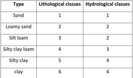
3.6 - Identify codes for the lithological and the hydrological classes assigned for the different materials in the ground of the considered Area ………52 3.7 - CN value for each kind of field ……….…………54 3.8 - Wilting point and field capacity for each of the 6 lithological classes ………54 3.9 - Values of the field capacity, wilting point and depth of the ground for each of the seven sub-regions ………55 3.10 - Final results of Thornthwaite’s model, percentage of infiltration for the 7 Thiessen polygons and average value within the entire Big Scale model ………56 3.11 - Resume of all the terms involved in the hydrological balance ………59 4.1 - Interval of variation for the five parameters and for the two chosen boundary conditions for the implementation of the sensitivity analysis ……….62 4.2 – Rankings obtained for the two methods of Morris’ and Sobol’ in the Composite Medium case. Morris has a sample size equal to 240 while Sobol equal to 2437 …………93 4.3 – Rankings obtained for the two methods of Morris’ and Sobol’ in the Overlapping Continua case with arithmetic average. Morris has a sample size equal to 240 while Sobol equal to 2437 ………93 4.4 – Rankings obtained for the two methods of Morris’ and Sobol’ in the Overlapping Continua case with geometric average. Morris has a sample size equal to 240 while Sobol equal to 2437 ……….94 5.1 – Results obtained for a calibration done over the five parameters in an Overlapping Continua case with arithmetic average. For each parameter is reported the material it represents, the initial value and the bounds it has for the calibration and the esteemed value with the bound of uncertainty obtained. It is a proof of the bad results which are obtained calibrating all the five conductivities ………97

XIII

5.2 – Bounds between which the parameters can vary during the calibration …………..97 5.3 – Set of values for each boundary conditions used for the calibration of all the conceptual models. As lower, intermediate and upper case we took the respective value of the interval used for the sensitivity analysis of these two boundary conditions ………..………..………..………..………..………..……….98 5.4 – Calibration results obtained with these starting values in the Composite Medium case with the three-different set of values of the boundary conditions. These results have been obtained for k1, k3 and k5 (the E. in the column “case” stands for “estimated”)

as k2 and k4 resulted not influent from the Sensitivity analysis (the F. in the column “case”

stands for “fixed”). The calibration has been done over the 40 hydraulic head measurement points ………..100 5.5 – Calibration results obtained with these starting values in the Overlapping Continua with arithmetic average case with the three-different set of values of the boundary conditions. These results have been obtained for k3 and k5 (the E. in the column “case”

stands for “estimated”) as k1, k2 and k4 resulted not influent from the Sensitivity analysis

(the F. in the column “case” stands for “fixed”). The calibration has been done over the 40 hydraulic head measurement points ………110 5.6 – Calibration results obtained with these starting values in the Overlapping Continua with geometric average case with the three-different set of values of the boundary conditions. These results have been obtained for k1, k3 and k5 (the E. in the column

“case” stands for “estimated”) as k2 and k4 resulted not influent from the Sensitivity

analysis (the F. in the column “case” stands for “fixed”). The calibration has been done over the 40 hydraulic head measurement points ……….120 5.7 - Values of the final objective function PHI and model validation criteria results for the three conceptual models in the BC1, BC2 and BC3 cases ……….129

1

ABSTRACT

The aim of this thesis is to test the applicability of two strategies, namely Composite and Overlapping continua Medium, to identify the key parameters affecting the dynamics of the subsurface at the field scale. The field site here considered is located in the Cremona region in the north of Italy.

The first step accomplished during this thesis has been the composition and analysis of an exhaustive dataset, describing the features of the study area. The lithological reconstruction of the study area has been performed clustering the geomaterials into five classes: silt and clay, sand, gravel, compact conglomerates and fractured conglomerates. Three different techniques have been implemented to reconstruct the spatial distribution of geomaterials: (1) The Composite Medium approach where each cell in which the aquifer is subdivided in formed by one single geomaterial, and the Overlapping Continua approach, where each cell of the domain is considered to be formed by a percentage of the 5 geomaterials and the overall conductivity is computed as a weighted (2) arithmetic or (3) geometric average of the conductivity of each geomaterial. For each of these three methods, two sensitivity analysis have been used to study the effect of each (and joint) parameter uncertainty on the uncertainty of model outputs. This analysis allows to select the key quantities (including parameters of the system and boundary conditions) that need to be accurately estimated for a reliable representation of the aquifer system. Then each selected model have been calibrated within a Maximum Likelihood approach considering only the key parameters affecting the system. Finally, we employ model validation criteria to select (or rank) amongst models.

2

Questo progetto di tesi si sviluppa all’interno del progetto WE-NEED (WatEr NEEDs, availability, quality and sustainability, www.we-need.polimi.it), finanziato dall’Unione Europea e dal Ministero Italiano dell’istruzione, dell’Università e della Ricerca (Water Joint Programming Initiative, 2015 Joint Call WaterWorks2014). WE-NEED ha lo scopo di sviluppare nuove strategie per l’uso sostenibile della risorsa idrica sotterranea.

Lo scopo di questa tesi è quello di analizzare l’influenza di diversi parametri in un modello di flusso delle acque sotterranee per un acquifero localizzato nella zona tra le provincie di Cremona e Bergamo. Questa regione è stata scelta come oggetto di studio in quanto caratterizzata dalla presenza dei cosiddetti fontanili; sorgenti d’acqua naturali che rappresentano una realtà naturalistica da preservare. Queste risorgive sono a forte rischio di contaminazione e di estinzione in quest’area.

Il primo passo effettuato per lo sviluppo di questo modello è stato quello della ricerca dati; un processo lungo e di rilevante importanza per l’intero svolgimento del progetto. Per la ricostruzione litologica della zona sono state individuate cinque classi di geomateriali: limi e argille, sabbia, ghiaia, conglomerati compatti e conglomerati fratturati. Con metodi geostatistici è stato possibile ricostruire la distribuzione di questi geomateriali all’intero dell’acquifero. Sono poi state utilizzate tre diverse concettualizzazioni del campo di conduttività: (1) Mezzo Composito e Mezzo a Continui multipli con media (2) aritmetica o (3) geometrica. Il Mezzo Composito consiste nel ritenere una singola cella del modello in cui l’acquifero è discretizzato occupata da un singolo geomateriale (quello in percentuale più presente nella cella stessa), mentre il metodo di Continui Multipli consiste nel considerare ogni cella costituita da piu’ geomateriali e quindi valutare la conduttività di ogni cella come media pesata (aritmetica o geometrica) delle conduttività di ogni geomateriale all’interno della cella. Ad ognuno dei tre modelli concettuali sviluppati, sono state applicate due diverse tipologie di analisi di sensitività con lo scopo di studiare quali siano i parametri del modello che maggiormente influiscono sulla distribuzione finale dei livelli piezometrici (output del modello) in corrispondenza dei punti di misura disponibili. I metodi utilizzati sono stati l’analisi basata sugli indici di Morris e di Sobol. Gli indici di Morris permettono

3

parametri e l’interazione tra essi. I parametri di cui è stata studiata l’influenza sono stati i valori di conduttività idraulica assegnata alle classi di geomateriali che compongono l’acquifero e due condizioni al contorno: il flusso di acqua in ingresso dal confine Nord del modello e l’altezza dei fiumi rappresentanti i confini Est, Ovest e Sud dell’area di interesse.

I risultati delle analisi di sensitività sono quindi stati utilizzati per la calibrazione delle conduttività idrauliche, considerando soltanto i parametri ritenuti più influenti dall’analisi di sensitività. La calibrazione utilizza il maximum likelihood ed è stata effettuata su 40 punti di cui erano disponibili osservazioni di carico idraulico.

Si è proceduto con la calibrazione per tutte e tre le ricostruzioni litologiche e per tre diversi valori in input delle condizioni al contorno di cui, precedentemente, è stata studiata la sensitività. I valori utilizzati per queste condizioni sono stati i limiti inferiori, superiori e il centro di banda dell’intervallo utilizzato per lo studio degli indici di Morris e Sobol. Sono quindi stati calibrati un totale di 9 modelli.

Questi modelli sono stati quindi confrontati tramite l’utilizzo di quattro model validation criteria. Questa analisi ha permesso di evidenziare che il modello il quale interpreta al meglio la risposta del sistema è il modello dei Continui Multipli con media aritmetica associando alle due condizioni al contorno sopra citate il valore relativo al limite superiore di banda dell’intervallo utilizzato.

4

1. INTRODUCTION

1.1

INTRODUCTION

The need of water due to the increase of the population and the pursuit of improved living conditions is a very actual matter nowadays. Water is a limited resource which, most of the time, is overused not thinking about the consequences linked to the losses of it. Most of the used one is groundwater, a strategic resource for human supplies, quite easy to reach and use. In large zone of the world the groundwater is the only available source of water humans have, hence it is over-exploited to sustain the necessity of the population living there. An excessive exploitation of groundwater could depauperate the surface water heritage, including all the environment linked to it. The over-exploitation it is not the only problem these sources have, because pollution is becoming more and more important, influencing not only the water itself, but all the environment. The more the population grows, the more will be the demand of water from these sources, leading to critical environmental, sociological and economic consequences.

No sustainable development can be reached unless the balance between demand and supply is achieved. Right now, the allowed amount of water which could be exploited from a source is theoretically equivalent to the all amount of water of the water body has itself [Gandolfi,2007]. This is the reason why over-exploitation is at the core of legal debates about water rights and is becoming an issue more and more actual and important.

The hydraulic withdraw evaluation sustainability level from the underground it is not possible with the normal investigations done for the concessions to new wells excavation and neither can be limited to the creation of a databank of the concessions themselves. To fix criterions to apply for a correct carrying out of the inquiries related to the questions of new concessions of derivation and withdrawals, the scientific world can furnish tools of support to the decisions. With the science, the hydraulic situation of the environment can be reproduced so that it can be possible to represents the evolution in time of the zone and to prevent some effect that derivations can cause in some zones.

5

Mathematical models are these tools of support to the decisions, and, in this specific case, it is needed a mathematical model of flow that integrates the knowledge of both the aquifer system and the hydrographical network of the surface.

This master thesis is inserted inside a bigger project which sees the collaboration of different universities, such as the Politecnico di Milano, the Weizmann Institute of Science, the Universidade de Aveiro and the Universitat Politecnica de Catalunya. The name of this project is WE-NEED (WatEr NEEDs, availability, quality and sustainability) and it has the aim to create an aquifer development providing an effective governance perspective while maximizing ecosystem preservation. More specifically WE-NEED will address the following aspects: over-exploitation of resources, interaction between all the system components, quality of both ground and surface water, study of the nature, the pathways and the ecotoxicological aspects that contaminants have, and social awareness. WE-NEED focuses the attention over two pilot areas with the purpose to have a model which is extendable to other threatened aquifers in Europe and worldwide. These two-pilot areas are different but complementary, and they are the aquifer of Cremona and Bologna, in the Padana plane in the north of Italy. These two sites are two distinct realities of alluvial aquifers and they can be representative of diverse environmental settings in Europe. Both sites are heavily exploited for different uses and are in risk of high contaminations.

This thesis is just a little part of all the work whom has to be done for the accomplishment of the aim WE-NEED has and it regards the creation and the study of the flux model in the Cremona region, characterized by the so-called springs belt. Natural springs have remarkable social, historical and touristic value and they are the main supply to agriculture and a key environmental driver. The following paragraph will largely explain these springs and the problems related to them.

This master thesis will use a previous mathematical model that was used for the same zone that will be studied, and it will analyse the various parameters that characterize the model by doing some sensitivity analysis, actualizing all the boundary conditions with recent values observed in the zone of interest. It will also add another case between the two conceptual models already used for the interpretation of the geomaterials. This chapter presents a description of the problem and how it is intended to solve it. Chapter 2 will explain the codes used for the implementation of the model and the

6

techniques of calibrations both in a mathematical and a computational point of view. It will also explain the model validation criteria used to choose the best model between the different used ones. Chapter 3 explains the two conceptual models that were used to create the aquifer under a mathematical point of view and all the computations and the new values used for the boundary conditions to run the model. In Chapter 4 the results of the two-sensitivity analysis explained in Chapter 2 are reported. Finally, Chapter 5 reports the model results obtained after a calibration done over those parameters resulted influencing from the sensitivity analysis of the previous chapter. It is in this last part that the results of the model validation criteria are shown.

1.2

THE “NATURAL SPRINGS BELT” IN THE PADANA PLANE

A natural spring, or resurge, is a zone where water flows from an aquifer to the earth’s surface. The groundwater uses to travel through a network of cracks and fissure and it tends to emerge following the outcropping of the less permeable layers. The forcing of the spring to the surface could be the result of a confined aquifer in which the water table of the spring stays at a higher elevation than that of the outlet. The out coming water is usually very pure and often, very close to the point of spill, it allows the formation of an uncontaminated environment. Coming from the underground, these waters have a temperature that around all the year is always maintained between 10°C and 14°C, allowing the use of the water also in the winter period because they don’t freeze. This continue availability of water is the reason why the agricultural activity around zones where these are presents it has always been so rich and active.

The “natural springs belt” is a hydrological formation typical of the northern part of the Padana plane, right at the feet of the Italian Alps, and it goes from Turin to Friuli-Venezia-Giulia passing by the Lombardia region for all its length. Is right in this zone that lot of resurges are active and they have been always used to allow the increasing of human activities.

7

Figure 1.1 – Some natural springs in the Lombardia region

In the Lombardia region this belt defines, approximately, two different zones: the northern and the southern zone with respect to this string.

 The northern zone is characterized by an intense consume of the ground in favour of the urbanization works, such as structures and infrastructures. The agriculture in this zone is important but mostly focused on specialized and industrial conductivities. This northern part causes two negative effects that influence the southern activities: first, the excessive urbanization is causing an increasing of the impermeable surfaces which distorts the water flux and then, because of this, the refill of the aquifer system it is no more sufficient to keep the whole system uncompromised.

 The southern zone of the natural spring string takes most of the water from the string itself and this area is mostly focused on agricultural purposes. This zone is the real engine of the dairy production of the whole Lombardia region.

8

Figure 1.2 – Scheme of the Padana Plane

The story of these natural springs is even more ancient than the irrigation practice itself, the main reason why these elements are used today. Long time ago all this area was nearly a swamp whose drainage let, with a lot of probability, the formation of this natural spring system. Nowadays the natural springs of this zone could be considered almost artificial because is the men’s activities who allows the spill of waters by cleaning all the interested area from possible cause of stick; and is always human the activity which let the water coming out from this points to flow away to be reused for different uses.

As it is understandable from what it is written just above, the life of this natural elements are strictly connected with human activities and life. Humans must take care of these natural springs while natural springs let human life to proceed normally, allowing the typical activities of the zone. The cleaning activity, directs to remove vegetation around the spill points, has a high cost which is covered until when the water coming out from the spring is enough to cover the cost of the maintenance. For this reason, when this amount decreases under a certain level, even if it’s sufficient to sustain the life of the environment around the source point, the economic interest around the maintenance is abandoned.

This problem linked to the cleaning and the maintenance of the natural springs is not the only one causing a possible failure of the system, there are a lot of other factors which could influence the life of a resurge. The principal causes linked to the degradation of this element could be:

9

 Decreasing of the water table around the point because of an excessive pumping out;

 Decreasing of the rain events;

 A complete landfill of the natural spring so that the entire ground could be used for agricultural purpose;

 Growing of vegetation around the point of spill as it was already explained before;

 Difficulties linked to the price of maintenance;

 Nowadays the extraction of water is more and more provided by private wells and the natural sources are being always more neglected.

Today this belt is keeping on reducing and it moves little by little the limit to the north. Some simple remedies could be done to save these elements:

 Determining a buffer zone where to avoid the realisation of superficial wells. The water of a natural springs it spills in that determine spot because there is a certain pressure and flow; if around this point there is something that could cause a perturbation of this situation, it should be avoided;

 Help with public money the maintenance of this environments without leaving these problems only to farmers and men working on these fields, since it is a public issue.

 Create a mathematical model which could reproduce the real situation of this entire zone so that the whole area could be monitored keeping the input and the output always actualized. This could help the authorities to give the permission of exploitation keeping in mind the preservation of the environment.

1.3

DEVELOPPING OF THE MODEL

The use of mathematical models in fields concerning the flux and the transport in natural systems in very common. A mathematical model is the description of a system using mathematical concepts and language. It is the simplification and it tries to simulate the answers of real systems and phenomenon involved in them. A model may help to explain a system and to study the effects of different components making predictions about

10

behaviours. Considering natural aquifers, some examples of external solicitations may be the pumping out from wells, phenomenon of contamination and recharges coming from rain or other kind of elements. All these are called, in a mathematical language, boundary conditions. The answer is typically a spatial or temporal variation in the distribution of the water head or either the concentration of some specific solute. Generally speaking, a mathematical model is divided in the following steps:

1. Defining the objectives to reach;

2. Implementation of the conceptual model of the system; 3. Choice or Implementation of the numerical code; 4. Implementation of the mathematical model;

5. Sensitivity analysis and Calibration of the parameters influencing the model. With the first step is also associated the phase of acquisition and organization of the information available around the specific subject to be studied. This is a very delicate phase because usually requires time and attention considering that data are given in different scales of observation. Another problem linked to this one could be the reliability or the distribution of data around the whole area of interest. All these elements are then transferred within a mathematical model in the same way and shape the code requires. Usually the natural system is discretized in the so-called cells where all the mathematical laws describing the specific model are computed for each one of them. It is convenient that the spatial discretisation of the grid is chosen considering the characteristics of the entire domain so that the error could be the less wide as possible. It is very common to increase the number of cells, so decreasing the size of them, in those zones where the dependant variables are subjected to higher variations. These grid refinements are used very often and typically in irregular limits.

To proceed with all the analysis, the spatial distribution of all the parameters acting in the model must be known. These parameters are fundamental because they are the elements over which all the mathematical equations describing the phenomenon are based. Therefore, at the beginning of the implementation of a model it is necessary to characterize it finding the right distribution of these parameters. These geological characteristics of natural formations can be very hard to compute because they vary considering the sampling point or either the scale of the model. Usually field or

11

laboratory tests are used in order to find them. From literature, it has been proposed to consider this input parameters as aleatory processes.

After having implemented the entire model, a calibration as to be done. This procedure makes sure that the specific model correctly describes the relationship between inputs and outputs. The adoption of this method let solve an inverse problem modifying with iterations the inputs (conductivities, fluxes, recharges, etc.…) until the minimization of a specific objective function is obtained.

This master thesis is all focused on the actualization and amelioration of a mathematical model that has been already developed over a specific zone of the northern Italy to prevent and study the problems linked to the activity of natural springs explained before. This was based over two conceptual models used to characterized all the parameters describing the area.

The first conceptual model it has been called Composite Medium and is based on the idea that the system is composed by lithological units different from one another, each of them characterized by his own hydraulic properties such as the hydraulic conductivity.

A second conceptual model is based on the idea that the system could be modelled considering the coexistence of different lithological units interacting one with another. Therefore, for each cell the system is divided into, all the parameters are computed considering a weighted average based on the percentage of the different materials present in it. This conceptual model will be called as Overlapping Continua.

The geo-materials that have been selected in order to proceed with the implementation of the mathematical model are just five. So the Overlapping Continua case does the average in a cell of all the values assigned to each one of the five categories basing on the percentage within that specific cell, while the Composite Medium case have just five kind of cells, because it assumes that all the cell is occupied by just one of the five geo-materials selected.

As said before these two methods were already implemented in another project concerning the same zone that this thesis re-take. All the parameters will be actualized with the more recent values obtained by observations of the past years and some sensitivity analysis will be done over the parameters influencing the whole model. Another contribute this thesis add is the study of the lithological model with another

12

kind of mathematical average. In fact, if the Overlapping Continua case was implemented only thinking about the classical weighted arithmetic average, in this master thesis it has been modelled also the lithological field with the weighted geometrical average, so that even the lower conductivities characterizing the ground could result important.

13

2. THEORETICAL BACKGROUND

2.1 GROUNDWATER FLOW MODEL

A wide range of groundwater flow model can be chosen to accomplish the aim explained in chapter 1. For this master thesis, it has been used the one called MODFLOW. MODFLOW is a very practical numeric code which can solve three-dimensional groundwater flow and contaminant transport simulation within a porous media with a finite-different method [Harbaugh,2005]. It is internationally known for the simulation and the prediction of groundwater conditions and groundwater or surface-water interactions. MOFLOW can simulate steady or unsteady flow in different kind of situation such as layers which are confined, unconfined or a combination of the two. It can simulate the flow coming from wells, different kind of recharges, evapotranspiration, drains or rivers. The version that has been used for this master thesis in the MODFLOW 2005 v.1.12.00, a standard one supported by the USGS Office of Groundwater and is the most modern, stable and well-tested version of the code. This version makes use of Fortran 90 programming language for storing and sharing data. The partial-differential equation used by MODFLOW 2005 which describes the three-dimensional movement of ground water through porous earth material is:

𝜕 𝜕𝑥(𝐾𝑥𝑥 𝜕ℎ 𝜕𝑥) + 𝜕 𝜕𝑦(𝐾𝑦𝑦 𝜕ℎ 𝜕𝑦) + 𝜕 𝜕𝑧(𝐾𝑧𝑧 𝜕ℎ 𝜕𝑧) + 𝑊 = 𝑆𝑠 𝜕ℎ 𝜕𝑡

Where 𝐾𝑥𝑥, 𝐾𝑦𝑦 and 𝐾𝑧𝑧 are the values of the hydraulic conductivity along the x,y and z

of the principal coordinates axes (L/T), h is the potentiometric head (L), W is a volumetric flux per unit volume representing sources or sinks within the system (T-1_{), 𝑆}

𝑠 is the

specific storage of the porous material (L-1_{) and, finally, t is the time (T).}

Except for very simple cases, analytical solutions of this equation are rarely possible and therefore usually a finite-difference method is used. With this methodology, the continuous system described by the equation is substitute by a set of discrete points in space and in time, and the partial derivatives are replaced by terms calculated from the differences in head values at these points. The head values of the cells are calculated in

14

a point called “node”; the finite-difference equation developed by MODFLOW individualize this node in the exact centre of the cells.

2.1.1 FINITE-DIFFERENCE EQUATION

Under the assumption that the sum of all flows coming in and out from a cell must be equal to the rate of change in storage in the cell and considering as constant the density of the groundwater, the continuity equation which describes the balance of flow for a cell is

∑ 𝑄_𝑖 = 𝑆𝑆∆ℎ

∆𝑡∆𝑉 (2.1) 𝑄_𝑖 is the flow rate entering a cell (L3_T-1_{), SS expresses the specific storage, so it is the}

volume of water that can be injected per unit volume of aquifer material per unit change in head (L-1_{). Finally, ∆𝑉 represents the volume of the cell (L}3_{) while ∆ℎ is the variation}

in the water head over a time interval ∆𝑡. Let’s consider a six aquifer cells as follows:

Figure 2.1 – Six adjacent cells around the cell i,j,k. (Representation from McDonald and Harbaugh,1988).

i,j+1,k i+1,j,k i,j-1,k i,j,k-1 i,j,k+1 i-1,j,k

15

Looking more precisely to two of the represented cells, the situation is as follows

Figure 2.2 – Flow coming from cell i,j-1,k into cell i,j,k.

Considering positive the flow entering in the cell i,j,k and then dropping the negative sign in the Darcy’s law from all terms, the flow into cell i,j,k in the row direction from cell i,j-1,k is given by the Darcy’s law as follows

𝑞𝑖,𝑗−1,𝑘 = 𝐾𝑅𝑖,𝑗−1/2,𝑘𝛥𝑐𝑖𝛥𝑣𝑘

(ℎ_{𝑖,𝑗−1,𝑘}− ℎ_{𝑖,𝑗,𝑘})

𝛥𝑟𝑗−1/2 (2.2)

ℎ_{𝑖,𝑗,𝑘} is the head at the node i,j,k while ℎ_{𝑖,𝑗−1,𝑘} the head in the node I,j-1,k.

𝑞_{𝑖,𝑗−1,𝑘}represents the volumetric flow rate through the face between cells i,j,k and

I,j-1,k (L3_T-1_{). 𝐾𝑅}

𝑖,𝑗−1/2,𝑘is the hydraulic conductivity along the row between nodes i,j,k and

i,j-1,k (LT-1_{),while 𝛥𝑐}

𝑖𝛥𝑣𝑘is the area of the surface normal to the row direction and

𝛥𝑟_𝑗−1/2 is the length between nodes i,j,k and i,j-1,k (L).

This equation gives the exact flow form for a one-dimensional steady-state case. This equation can be written for all the cases of the six cells represented. These remaining five equations are:

𝑞𝑖,𝑗+1/2,𝑘= 𝐾𝑅𝑖,𝑗+1/2,𝑘𝛥𝑐𝑖𝛥𝑣𝑘 (ℎ𝑖,𝑗+1,𝑘− ℎ𝑖,𝑗,𝑘) 𝛥𝑟_𝑗+1/2 (2.3) 𝑞_{𝑖+1/2,𝑗,𝑘} = 𝐾𝐶_{𝑖+1/2,𝑗,𝑘}𝛥𝑟_𝑖𝛥𝑣_𝑘(ℎ𝑖+1,𝑗,𝑘− ℎ𝑖,𝑗,𝑘) 𝛥𝑐_𝑖+1/2 (2.4) 𝑞𝑖−1/2,𝑗,𝑘 = 𝐾𝐶𝑖−1/2,𝑗,𝑘𝛥𝑟𝑗𝛥𝑣𝑘 (ℎ𝑖−1,𝑗,𝑘− ℎ𝑖,𝑗,𝑘) 𝛥𝑐_𝑖−1/2 (2.5) 𝑞_{𝑖,𝑗,𝑘+1/2} = 𝐾𝑉_{𝑖,𝑗,𝑘+1/2}𝛥𝑟_𝑗𝛥𝑐_𝑖(ℎ𝑖,𝑗,𝑘+1− ℎ𝑖,𝑗,𝑘) 𝛥𝑣_𝑘+1/2 (2.6) i,j-1,k i,j,k 𝑞𝑖,𝑗−1/2,𝑘 𝛥𝑟𝑗 𝛥𝑟_𝑗−1/2 𝛥𝑣𝑘 𝛥𝑐𝑖 𝛥𝑟_𝑗−1

16

𝑞_{𝑖,𝑗,𝑘−1/2} = 𝐾𝑉_{𝑖,𝑗,𝑘−1/2}𝛥𝑟_𝑗𝛥𝑐_𝑖(ℎ𝑖,𝑗,𝑘−1− ℎ𝑖,𝑗,𝑘)

𝛥𝑣_𝑘−1/2 (2.7)

These notations can be simplified using the “hydraulic conductance”, a combination of grid dimensions and hydraulic conductivity. The conductance can be expressed as

𝐶𝑅𝑖,𝑗−1/2,𝑘 =

𝐾𝑅_{𝑖,𝑗−1/2,𝑘}𝛥𝑐_𝑖𝛥𝑣_𝑘

𝛥𝑟_𝑗−1/2 (2.8) The conductance is the product of hydraulic conductivity and cross-sectional area of flow all divided the distance of the flow path. In this case 𝐶𝑅_{𝑖,𝑗−1/2,𝑘} is the conductance in row i and layer k between cells i,j-1 and i,j,k (L2_T-1_{). Knowing this, all the equations}

written before can be expressed as 𝑞_{𝑖,𝑗−1/2,𝑘}= 𝐶𝑅 𝑖,𝑗−1₂,𝑘(ℎ𝑖,𝑗−1,𝑘− ℎ𝑖,𝑗,𝑘) (2.9) 𝑞𝑖,𝑗+1/2,𝑘= 𝐶𝑅_𝑖,𝑗+1 2,𝑘 (ℎ𝑖,𝑗+1,𝑘− ℎ𝑖,𝑗,𝑘) (2.10) 𝑞_{𝑖−1/2,𝑗,𝑘} = 𝐶𝑅_{𝑖−1/2,𝑗,𝑘}(ℎ_{𝑖−1,𝑗,𝑘}− ℎ_{𝑖,𝑗,𝑘}) (2.11) 𝑞𝑖+1/2,𝑗,𝑘 = 𝐶𝑅𝑖+1/2,𝑗,𝑘(ℎ𝑖+1,𝑗,𝑘− ℎ𝑖,𝑗,𝑘) (2.12) 𝑞_{𝑖,𝑗,𝑘+1/2} = 𝐶𝑅_{𝑖,𝑗,𝑘+1/2}(ℎ_{𝑖,𝑗,𝑘+1}− ℎ_{𝑖,𝑗,𝑘}) (2.13) 𝑞_{𝑖,𝑗,𝑘−1/2} = 𝐶𝑅_{𝑖,𝑗,𝑘−1/2}(ℎ_{𝑖,𝑗,𝑘−1}− ℎ_{𝑖,𝑗,𝑘}) (2.14)

To consider flows coming from external processes such as rivers, drains, evapotranspiration, recharges, wells or others, additional terms should be added to the equation. All these terms could be dependent on the head in the cell or entirely independent of it. Considering that there are N external sources affecting a cell, the expression in order to account these external stresses is the following

∑ 𝑎_{𝑖,𝑗,𝑘,𝑛} 𝑁 𝑛=1 = ∑(𝑝_{𝑖,𝑗,𝑘,𝑛} 𝑁 𝑛=1 ℎ_{𝑖,𝑗,𝑘}) + ∑ 𝑞_{𝑖,𝑗,𝑘,𝑛} (2.15) 𝑁 𝑛=1

The flow coming from the nth external source is represented by the term 𝑎_{𝑖,𝑗,𝑘,𝑛} (L3_T-1₎

while 𝑝𝑖,𝑗,𝑘,𝑛 and 𝑞𝑖,𝑗,𝑘,𝑛 are constants, respectively (L2T-1) and (L3T-1). These two terms

17 𝑃𝑖,𝑗,𝑘 = ∑ 𝑝𝑖,𝑗,𝑘,𝑛 𝑁 𝑛=1 (2.16) 𝑄𝑖,𝑗,𝑘 = ∑ 𝑞𝑖,𝑗,𝑘,𝑛 𝑁 𝑛=1 (2.17) So that the general from for the external flow for a single cell i,j,k is

∑ 𝑎𝑖,𝑗,𝑘,𝑛 𝑁

𝑛=1

= 𝑃𝑖,𝑗,𝑘ℎ𝑖,𝑗,𝑘+ 𝑄𝑖,𝑗,𝑘 (2.18)

The continuity equation, considering the six contributes coming for the six adjacent cells and the external flow rate can be expressed as

𝑞

𝑖,𝑗−1₂,𝑘 + 𝑞𝑖,𝑗+1₂,𝑘+ 𝑞𝑖+1₂,𝑗,𝑘+ 𝑞𝑖−1₂,𝑗,𝑘+ 𝑞𝑖,𝑗,𝑘+1₂ + 𝑞𝑖,𝑗,𝑘−1₂+

+𝑃_{𝑖,𝑗,𝑘}ℎ_{𝑖,𝑗,𝑘} + 𝑄_{𝑖,𝑗,𝑘} = 𝑆𝑆_{𝑖,𝑗,𝑘}(𝛥𝑟_𝑗𝛥𝑐_𝑖𝛥𝑣_𝑘)𝛥ℎ𝑖,𝑗,𝑘

𝛥𝑡 (2.19) Where 𝑆𝑆𝑖,𝑗,𝑘 is the specific storage of cell i,j,k (L-1) while 𝛥𝑟𝑗𝛥𝑐𝑖𝛥𝑣𝑘 is the volume of cell

i,j,k (L3_{) and} 𝛥ℎ𝑖,𝑗,𝑘

𝛥𝑡 is the derivative of head with respect to time (LT

-1_{). This term can be}

written in a more precise way

∆ℎ𝑖,𝑗,𝑘

∆𝑡 ≅

ℎ_{𝑖,𝑗,𝑘}𝑚 − ℎ_{𝑖,𝑗,𝑘}𝑚−1

𝑡𝑚_{− 𝑡}𝑚−1 (2.20)

ℎ_{𝑖,𝑗,𝑘}𝑚 represents the head in the cell i,j,k at a time m, 𝑡𝑚 is the time at the temporal step

m, while ℎ_{𝑖,𝑗,𝑘}𝑚−1 and 𝑡𝑚−1 are the water head and the time at a previous time step. For a steady state condition this term is equal to zero, and so it is all the term to the right of the equal.

Finally this equation can be re-written for the finite-differences for a single cell i,j,k as 𝐶𝑅_𝑖,𝑗−1 2,𝑘 (ℎ𝑖,𝑗−1,𝑘− ℎ𝑖,𝑗,𝑘) + 𝐶𝑅_𝑖,𝑗+1 2,𝑘 (ℎ𝑖,𝑗+1,𝑘− ℎ𝑖,𝑗,𝑘) + +𝐶𝐶 𝑖−1₂,𝑗,𝑘(ℎ𝑖−1,𝑗,𝑘− ℎ𝑖,𝑗,𝑘) + 𝐶𝐶𝑖+1₂,𝑗,𝑘(ℎ𝑖+1,𝑗,𝑘− ℎ𝑖,𝑗,𝑘) + +𝐶𝑉_{𝑖,𝑗,𝑘−}1 2 (ℎ𝑖,𝑗,𝑘−1− ℎ𝑖,𝑗,𝑘) + 𝐶𝑉_{𝑖,𝑗,𝑘+}1 2 (ℎ𝑖,𝑗,𝑘+1− ℎ𝑖,𝑗,𝑘) + +𝑃_{𝑖,𝑗,𝑘}ℎ_{𝑖,𝑗,𝑘}+ 𝑄_{𝑖,𝑗,𝑘} = 𝑆𝑆_{𝑖,𝑗,𝑘}(𝛥𝑟_𝑗𝛥𝑐_𝑖𝛥𝑣_𝑘)𝛥ℎ𝑖,𝑗,𝑘 𝛥𝑡 (2.21)