POLITECNICO DI MILANO
Scuola di Ingegneria Industriale e dell'Informazione
Tesi di Laurea Magistrale in Ingenieria Biomedica
Assessment of spatial heterogeneity of ventricular
repolarization in patients with atrial fibrillation
Anno accademico 2017/2018
Relatori:
Prof. Luca T. Mainardi
Prof. Valentina Corino
Candidati:
Matr.
Francisco Javier Saiz Vivó, 2018
Assessment of spatial heterogeneity of ventricular repolarization in patients with atrial fibrillation.
Date: April 19th, 2018
This Master thesis has been developed within the Dipartimento di Elettronica, Informazione e Bioingegneria (DEIB) from Politecnico di Milano.
i
CONTENTS
Chapter 1. SUMMARY ... vii
Chapter 2. SOMMARIO ... xvii
Chapter 3. INTRODUCTION ... 1
Academic Motivation ... 1
Research Motivation ... 1
Heart ... 1
Cardiac Electrophysiology ... 4
Extracellular bioelectric potential signals ... 4
Electrical Activity of Normal Heart ... 5
ECG signal ... 6
The 12 Standard Leads... 7
Abnormal Cardiac Conditions ... 10
3.9.1 Atrial Fibrillation ... 11
3.9.2 AF Mechanisms ... 12
3.9.3 Types of AF ... 12
3.9.4 Atrioventricular nodal function during AF ... 13
𝓥-index ... 13
Objectives and Outline ... 16
Chapter 4. MATERIALS ... 17
Chapter 5. METHODS ... 19
AF Simulation ... 19
5.1.1 Add f-waves ... 21
ii
5.1.3 Calculate 𝓥-index ... 31
Study of Swiss AF database ... 31
5.2.1 Elimination of f-waves ... 32 5.2.2 Pre-processing ... 38 5.2.3 T-wave detection ... 38 Chapter 6. RESULTS ... 41 AF Simulation ... 41 Swiss-AF Study ... 48
6.2.1 AF patients with and without f-waves ... 48
6.2.2 SR patients and AF patients without f-waves ... 52
Chapter 7. DISCUSSION ... 59
Chapter 8. CONCLUSION AND FURTHER WORK ... 63
iii
LIST OF FIGURES
Fig. 1-1 T-waves for 12 Standard Leads. ... x
Fig. 1-2 T-waves for 12 Standard Leads with f-waves. ... x
Fig. 1-3 AF Simulation Comparisons for simulation frequency = 5Hz. ... xii
Fig. 1-4 Comparison between Paroxysmal patients in AF without f-waves and SR conditions ... xiv
Fig. 1-5 Comparison between Persistent and Permanent patients in AF conditions. ... xv
Fig. 2-1 Onde T senza onde fibrillatorie. ... xx
Fig. 2-2 Onde T con onde fibrillatorie. ... xx
Fig. 2-3 Valori Teorici contro valori Senza Onde fibrillatorie e valori Con Onde fibrillatorie, per i tre metodi e frequenza di simulazione 5 Hz. ... xxii
Fig. 2-4 Confronto tra Pazienti Parossistici con RS e con FA senza onde fibrillatorie. ... xxiv
Fig. 2-5 Confronto per i pazienti con FA Persistenti e Permanenti senza onde fibrillatorie. ... xxv
Fig. 3-1 Structure of the heart, and course of blood flow through the heart chambers and heart valves. From [3]. ... 2
Fig. 3-2 Summary of the two main heart stages: Systole and Diastole. From [4]. ... 3
Fig. 3-3 Effect of different ions in the phases of generation of AP. Modified from [5]. . 5
Fig. 3-4 Typical APs in the principal Cardiac Structures and their combined effect resulting in the ECG. From [6]. ... 6
Fig. 3-5 Normal Electrocardiogram. From [3]. ... 6
Fig. 3-6 Einthoven's Triangle. From www.medicine.mcgill.ca/physio/vlab/cardio/setup.htm. ... 8
Fig. 3-7 ECG waveforms depending on the lead. From [6]. ... 8
Fig. 3-8 Augmented Unipolar Leads. From http://www.cvphysiology.com/Arrhythmias/A013b. ... 9
Fig. 3-9 Placement of intercostal leads. From [7]. ... 10
Fig. 3-10 Wilson Central Terminal. Modified from [6]. ... 10
Fig. 3-11 Diagram of AF. From Mayo Foundation for Medical Education and Research. ... 11
iv
Fig. 3-13 Genesis of the T-wave. ... 13
Fig. 5-1 T-waves for 12 Standard Leads. ... 20
Fig. 5-2 Block Diagram of Processes in AF Simulation. ... 20
Fig. 5-3 dl (t),sl (t) and fl (t) for the 3 Orthogonal Leads and AF simulation frequency of 5 Hz. ... 22
Fig. 5-4 T-waves for 12 Standard Leads with f-waves. ... 23
Fig. 5-5 Dominant T-waves estimated with Method 1. ... 26
Fig. 5-6 Dominant T-waves estimated with Method 2. ... 27
Fig. 5-7 Dominant T-waves estimated with Method 3. ... 30
Fig. 5-8 Block Diagram of Processes in Swiss-AF Study. ... 32
Fig. 5-9 Original ECG signal with QRST start (red), QRS Peak (yellow) and QRST end (purple) marked. ... 34
Fig. 5-10 Original Signal and Zglob obtained from Atrial Fibrillation Reduction. ... 34
Fig. 5-11 Sample Beat with Rough T-wave Window used to compute T-wave delineator. ... 35
Fig. 5-12 Summary of T-wave delineator (Toff) on sample T-wave. ... 36
Fig. 5-13 Original ECG and ECG output without f-waves. ... 38
Fig. 5-14 Aligned T-waves using a Rough T-wave Window. ... 39
Fig. 5-15 Aligned T-wave with the new Ton and Toff from the T-wave delineator. ... 39
Fig. 6-1 AF Simulation Comparisons for simulation frequency = 3Hz. ... 41
Fig. 6-2 AF Simulation Comparisons for simulation frequency = 4Hz. ... 42
Fig. 6-3 AF Simulation Comparisons for simulation frequency = 5Hz. ... 42
Fig. 6-4 AF Simulation Comparisons for simulation frequency = 6Hz. ... 43
Fig. 6-5 AF Simulation Comparisons for simulation frequency = 7Hz. ... 43
Fig. 6-6 AF Simulation Comparisons for simulation frequency = 8Hz. ... 44
Fig. 6-7 AF Simulation Comparisons for simulation frequency = 9Hz. ... 44
Fig. 6-8 AF Simulation Comparisons for simulation frequency = 10Hz. ... 45
Fig. 6-9 AF Simulation Comparisons for simulation frequency = 11Hz. ... 45
Fig. 6-10 AF Simulation Comparisons for simulation frequency = 12Hz. ... 46
Fig. 6-11 Comparison between All AF patients with and without f-waves. ... 49
Fig. 6-12 Comparison between Paroxysmal AF patients with and without f-waves. .... 49
Fig. 6-13 Comparison between Persistent AF patients with and without f-waves. ... 50
Fig. 6-14 Comparison between Permanent AF patients with and without f-waves. ... 50
Fig. 6-15 Comparison between Paroxysmal patients in AF without f-waves and SR conditions. ... 52
Fig. 6-16 Comparison between Persistent patients in AF without f-waves and SR conditions. ... 53
Fig. 6-17 Comparison between Paroxysmal and Persistent patients in SR conditions. . 54
Fig. 6-18 Comparison between Paroxysmal, Persistent and Permanent patients in AF conditions. ... 55
Fig. 6-19 Comparison between Persistent and Permanent patients in AF conditions. ... 56
Fig. 7-1 Two cardiologists' marks of T-wave ends for 3 beats in a QT Dataset. The differences are 17ms (a), 15ms (b) and 104ms (c). From [45]. ... 60
v
LIST OF TABLES
Table 1-1 Mean Absolute Percentage Error between theoretical index values and
V-index values for T-waves with and without f-waves for Simulation Frequency 5 Hz. . xiii
Table 1-2 Median and Standard Deviation for the V-index values of the comparison and the Increase in Median between the values of the patients in AF without f-waves and SR conditions. ... xiv
Table 1-3 Median and Standard Deviation for the V-index values of the different comparisons, the Increase in Median between the values of the Persistent and Permanent patients in AF and the P value of those comparisons. ... xv
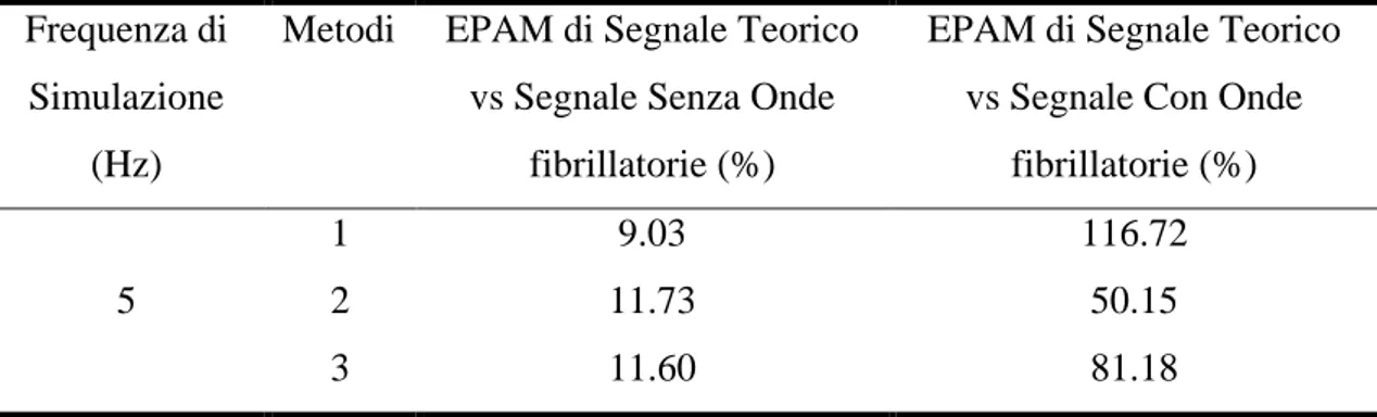
Table 2-1 EPAM di Segnale Teorico contro Segnale Senza Onde fibrillatorie e Con onde fibrillatorie, per i tre metodi e frequenza di simulazione 5 Hz. ... xxiii
Table 2-2 Indice V per Pazienti con RS e Pazienti con FA senza onde fibrillatorie per episodi Parossistici. ... xxiv
Table 2-3 Indice V per Pazienti con AF Persistenti e Permanente. ... xxv
Table 3-1 Usual duration of ECG intervals. ... 6
Table 3-2 Potential difference in Leads I, II and III. ... 8
Table 3-3 Placement of intercostal leads. ... 10
Table 4-1 Overview of the study procedures. Procedures for baseline have been highlighted. From [31]. ... 18
Table 5-1 Parameter values for simulating f-waves. From [34]. ... 21
Table 6-1 Mean Absolute Percentage Error between theoretical index values and V-index values for T-waves with and without f-waves. ... 46
Table 6-2 Median and Standard Deviation for the V-index values of the different comparisons and the Increase in Median between the values with and without f-waves. ... 51
Table 6-3 Summary of Patients. ... 52
Table 6-4 Median and Standard Deviation for the V-index values of the different comparisons and the Increase in Median between the values of the patients in AF without f-waves and SR conditions. ... 53
vi
Table 6-5 Median and Standard Deviation for the V-index values of the different comparisons, the Increase in Median between the values of the Paroxysmal and
Persistent patients in SR and the P value of those comparisons. ... 54 Table 6-6 Median and Standard Deviation for the V-index values of the Paroxysmal, Persistent and Permanent patients in AF conditions. ... 56 Table 6-7 Median and Standard Deviation for the V-index values of the different
comparisons, the Increase in Median between the values of the Persistent and
vii
Chapter 1. SUMMARY
Introduction
Atrial Fibrillation (AF) is the most common sustained arrhythmia encountered in clinical practice. The progressive aging of the general population is associated with an inevitable rising in incidence of this particular rhythm disorder which in 2005 alone was responsible for 193,300 deaths, up from 29,000 in 1990 [1][2]. In providing proper treatment, the clinician must establish the pattern of arrhythmia, determine associated symptoms, and asses for underlying comorbidities in order to define short- and long-term management strategies.
Although there is no common agreement today on the best AF classification, current clinical guidelines advocate differentiating between paroxysmal, persistent and permanent AF [9].
1. Paroxysmal AF: AF with spontaneous interruption generally within 7 days but mostly in 24-48 h,
2. Persistent: AF that does not interrupt spontaneously but with therapeutic interventions (pharmacological or electrical), and
3. Permanent or chronic AF: AF in which interruption attempts have not been made or, if made, have not been successful.
One of the objectives of this thesis is to try to discriminate between the 3 types of AF. The spatial dispersion of ventricular repolarization is responsible for the genesis of the T-wave on the ECG therefore, based on van Oosterom’s take on Dominant T-T-wave formalism (DTW) and its derivatives, a novel method to quantify the dispersion of myocytes’ repolarization times, rooted on a biophysical model of the ECG called the
viii
𝒱-𝑖𝑛𝑑𝑒𝑥 was derived. The 𝒱-𝑖𝑛𝑑𝑒𝑥 is an electrocardiogram (ECG)-based estimator of the standard deviation of ventricular myocytes’ repolarization times, 𝑠𝜗.
Specifically, the 𝒱-𝑖𝑛𝑑𝑒𝑥 computes 𝑠𝜗 through the ratio of the standard deviations of the
lead factors measured across successive beats according to the following formula:
where 𝑤1(𝑖) and 𝑤2(𝑖) are the lead factors which are derived from:
where 𝛹𝐿×𝑁 is a matrix containing N ECG samples recorded from L leads, 𝑤1 and 𝑤2 are
2 sets of L x 1 vectors of leads factors, Td is a 1 x N vector obtained after sampling Ḋ(t) and Ṫd its derivative.
The objective of this thesis is the assessment of spatial heterogeneity of ventricular repolarization in patients with atrial fibrillation, which includes:
Simulation: use physiological T-waves to study the differences that arise in the 𝒱-𝑖𝑛𝑑𝑒𝑥 in 3 cases:
o Theoretical case
o Sinus Rhythm condition o Atrial Fibrillation condition
The AF condition was achieved by adding simulated f-waves to the physiological T-waves using the method described in [34].
Study of Swiss AF database: compute and compare the 𝒱-𝑖𝑛𝑑𝑒𝑥𝑒𝑠 of 2013 patients in paroxysmal and persistent SR and Paroxysmal, Persistent and permanent AF, in the 3 main 𝒱-𝑖𝑛𝑑𝑒𝑥 computation methodologies.
Materials
For this thesis, Swiss Atrial Fibrillation (Swiss-AF) cohort carried out a study of 2400 patients across 13 sites in Switzerland. Out of the ECG signals of the 2400 patients, 2013 had signals clear enough to conduct the computation of the 𝒱-𝑖𝑛𝑑𝑒𝑥, out of which 902 patients present paroxysmal, 608 persistent and 503 permanent AF. Eligible
patients had to be ≥65 years old and had to have one of the 3 AF patterns studied. 𝒱𝑖 = 𝑠𝑡𝑑[𝑤2(𝑖)]
𝑠𝑡𝑑[𝑤1(𝑖)] ≈ 𝑠𝜗
(1-1)
SUMMARY
ix Main exclusion criteria included inability to provide informed consent, the presence of exclusively nonsustained episodes of secondary form of AF (e.g. after cardiac surgery or severe sepsis) or any acute illness within the last 4 week. The latter group of patients were eligible for enrolment after stabilization of their acute episode.
Methods
The methodology of this thesis is divided in two distinct stages: AF simulation and Study of Swiss-AF database.
AF simulation’s main processes are add AF, calculate w1 and w2 and calculate the V index of the theoretical values and the experimental values with and without f waves. Swiss-AF database’s main processes include Elimination of f-waves if necessary for AF patients, and then for all the patients: a Pre-processing stage which includes filtering and Baseline Alignment, the T wave detection stage which includes the use of Pan Tompkins algorithm to determine the position of the QRS, Rough Beat Alignment, T-Wave Delineation, Beat Re-Alignment and cross correlation to identify the good leads. Finally, as in the AF simulation, the stages of 𝑤1 and 𝑤2 and 𝒱-𝑖𝑛𝑑𝑒𝑥 calculation.
AF simulation
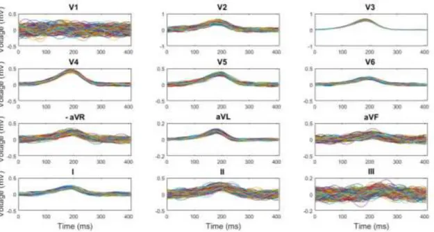
The AF simulation started with T-waves from the 12 Standard Leads and theoretical 𝑤1, 𝑤2 and 𝒱-𝑖𝑛𝑑𝑒𝑥 values for seven patients were used.
x
Fig. 1-1 T-waves for 12 Standard Leads.
To see the effect the f-waves had in the computation of the 𝒱-𝑖𝑛𝑑𝑒𝑥, fibrillatory waves were simulated and added to the T-waves following the steps described in [34]. Fig. 1-2 shows the T-waves with the added f-waves.
SUMMARY
xi For the experimental values both with and without f-waves, 𝑤1 and 𝑤2 must be calculated in order to calculate the 𝒱-𝑖𝑛𝑑𝑒𝑥. To do so, this thesis describes 3 different methods hereinafter Method 1, Method 2 and Method 3.
Method 1: estimate the dominant T-wave (DTW) of each beat. Method 2: estimating a single DWT, shared across beats.
Method 3: Sinusoidal functions to estimate the dominant T-wave.
Study of Swiss AF database
The main part of this thesis was the study of the Swiss-AF database, which divided the patients into 5 groups: AF (Paroxysmal, Persistent and Permanent) and SR (Paroxysmal and Persistent) in order to later do some comparisons between the 𝒱-𝑖𝑛𝑑𝑒𝑥 results obtained from each of the subgroups.
The processes followed in this stage include Elimination of f-waves in AF patients if necessary and then in all the patients: Pre-processing, T-wave detection, 𝑤1 and 𝑤2
calculation and 𝒱-𝑖𝑛𝑑𝑒𝑥 calculation. The processes 𝑤1 and 𝑤2 calculation and 𝒱-𝑖𝑛𝑑𝑒𝑥 calculation are analogous to the processes described in the AF Simulation stage.
In order to determine the necessity of eliminating the f-waves of the AF patients before computing the 𝒱-𝑖𝑛𝑑𝑒𝑥, the study of Swiss-AF database was divided into 2 sub-stages:
Comparison between AF patients with and without f-waves Comparison between AF and SR patients.
The AF patients of the second comparison will or will not have f-waves depending on the results obtained in the first comparison.
Elimination of f-waves
The method consisted on the pre-processing of the signal, T-wave detection, Atrial Fibrillation Reduction, Beat Averaging, Estimation of QRST Cancellation Parameters, QRST Cancellation and f-waves elimination.
T-wave detection
The T-wave detection was done by computing the maximum derivative and calculate a Reference Line, which is a straight line that passes through the point of maximum
xii
derivative and has a gradient equal to a fourth of the maximum derivative. The end of the T-wave is then determined by the point of the T-wave which has the maximum distance from the Reference Line.
Results
This section will describe the most relevant results obtained in the stages of this thesis: Simulation and Swiss-AF study.
Simulation:
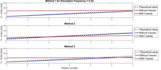
The simulation was done in order to determine if it was necessary to eliminate the f-waves from the AF patients before calculating the 𝒱-𝑖𝑛𝑑𝑒𝑥. Seven sets of T-waves were analysed and the theoretical 𝒱-𝑖𝑛𝑑𝑒𝑥 values were compared against the 𝒱-𝑖𝑛𝑑𝑒𝑥 of the T-waves with and without simulated f-waves. Fig. 1-3 and Table 1-1 show the results obtained for Simulation Frequency 5 Hz.
SUMMARY
xiii
Table 1-1 Mean Absolute Percentage Error between theoretical V-index values and V-index values for T-waves with and without f-T-waves for Simulation Frequency 5 Hz.
Simulation Frequency
(Hz)
Method Theoretical vs Signal without f waves MAPE (%)
Theoretical vs Signal with f waves MAPE (%)
5
1 9.03 116.72
2 11.73 50.15
3 11.60 81.18
The Mean Absolute Percentage Error (MAPE) for Theoretical vs Signal without f-waves are considerably lower than for Theoretical vs Signal with f-waves. The assumption that the f-waves affect the computation of the 𝒱-𝑖𝑛𝑑𝑒𝑥 is therefore proven and justifies the decision to make a previous Swiss-AF study in order to confirm the effect of f-waves in the computation of the V index in real ECG signals.
Swiss-AF Study
SR patients and AF patients without f-waves
The results obtained in the comparisons for SR patients and AF patients without f-waves are going to be presented.
Out of the 879 AF patients and 1134 SR patients, 772 AF and 1092 SR patients gave usable 𝒱-𝑖𝑛𝑑𝑒𝑥 results. The 772 AF patients include 135 with Paroxysmal, 217 with Persistent and 420 with Permanent fibrillatory episodes and the 1092 SR patients include 747 with Paroxysmal and 345 with Permanent episodes.
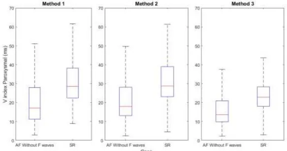
A comparison between SR patients and AF patients without f-waves was made for Paroxysmal and Persistent episodes. As an example, Fig. 1-4 shows the box plot obtained in the comparison of Paroxysmal episodes:
xiv
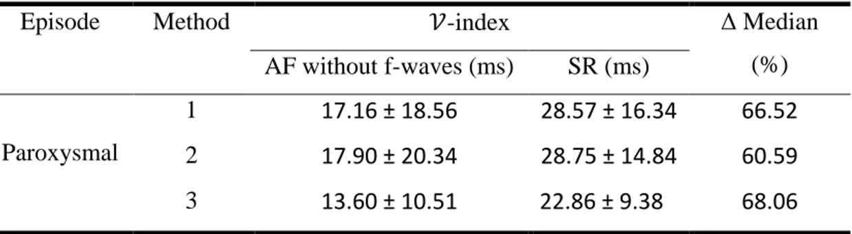
And Table 1-2 summarises the results:
Table 1-2 Median and Standard Deviation for the V-index values of the comparison and the Increase in Median between the values of the patients in AF without f-waves and SR conditions.
Episode Method 𝒱-index Δ Median
(%) AF without f-waves (ms) SR (ms) Paroxysmal 1 17.16 ± 18.56 28.57 ± 16.34 66.52 2 17.90 ± 20.34 28.75 ± 14.84 60.59 3 13.60 ± 10.51 22.86 ± 9.38 68.06
Both Fig. 1-4 and Table 1-2 show that there is an increase in the median of the 𝒱-𝑖𝑛𝑑𝑒𝑥 for patients during SR than for patients during AF without f-waves. This may be due to the fact that during fibrillation the ventricular myocytes’ repolarization times decreases. As one of the objectives was to be able to discriminate between Persistent and Permanent AF episodes, Fig. 1-5 shows the comparison between Persistent and Permanent patients in AF conditions.
SUMMARY
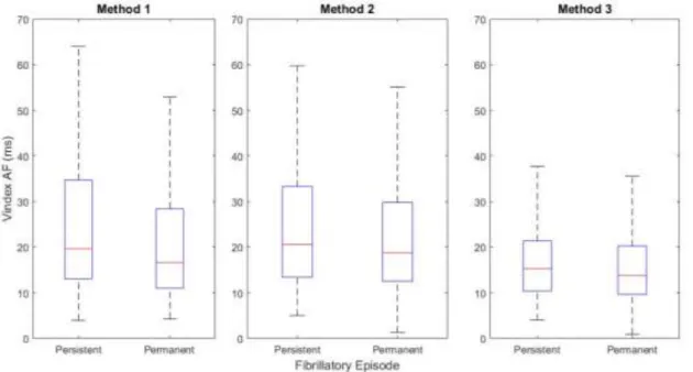
xv
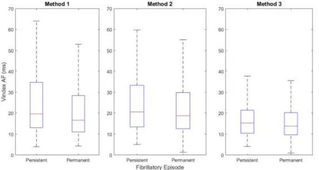
Fig. 1-5 Comparison between Persistent and Permanent patients in AF conditions.
A study was made on the statistical values of the 𝒱-𝑖𝑛𝑑𝑒𝑥 and its results are shown in Table 1-3.
Table 1-3 Median and Standard Deviation for the V-index values of the different comparisons, the Increase in Median between the values of the Persistent and Permanent patients in AF and the P value of those comparisons.
Method 𝒱-index Δ Median (%) P value ≤ 0.05
Persistent (ms) Permanent (ms)
1 19.65 ± 20.31 16.62 ± 17.03 18.23 0.01
2 20.57 ± 23.71 18.76 ± 16.99 9.69 0.02
3 15.30 ± 11.16 13.77 ± 9.31 11.08 0.03
The median of the 𝒱-𝑖𝑛𝑑𝑒𝑥 for patients with Persistent episodes is higher than for patients with Permanent episodes. Furthermore, for these comparisons, the null hypothesis was rejected when the P value ≤ α, with α = 0.05. The null hypotheses were rejected in all the comparisons and were deemed statistically significant as the P values of all the comparisons were ≤ 0.05.
From these values, one could argue that it is possible to discriminate between Persistent and Permanent episodes in patients with AF.
xvi
Conclusion
The assessment of spatial heterogeneity of ventricular repolarization in patients with atrial fibrillation was the aim of this thesis. The aim was met and the results have shown that:
the method used to estimate the lead factors 𝑤1 and 𝑤2 from the ECG introduce
bias in the 𝒱-index. However, throughout the comparisons, the standard deviation of the 𝒱-index for Method 3 was the lowest. This proves that the analytical form (with 5 being the number of Taylor terms) has a more reliable estimate [36]. there is a significant effect of the presence of f-waves when computing the
𝒱-index and thus, the fibrillatory component should be removed from the AF signals before the computation.
with some limitations, the methods developed for eliminating the f-waves and delineating the T-wave generally worked.
no statistically significant results were provided when trying to discriminate paroxysmal from persistent patterns in SR patients
in AF patients, the comparison between Persistent and Permanent patterns gave significant results as 𝑠𝜗 was higher for Persistent than for Permanent AF patients.
xvii
Chapter 2. SOMMARIO
Introduzione
La fibrillazione atriale (FA) è l'aritmia sostenuta più comune riscontrata nella pratica clinica. Il progressivo invecchiamento della popolazione generale è associato ad un inevitabile aumento dell'incidenza di questo particolare disturbo del ritmo che nel solo 2005 è stato responsabile di 193.300 decessi, contro i 29.000 nel 1990 [1] [2]. Nel fornire un trattamento adeguato, il dottore deve stabilire il modello di aritmia, determinare i sintomi associati e valutare le comorbidità sottostanti al fine di definire strategie di gestione a breve e lungo termine.
Anche se oggi non esiste un accordo comune sulla migliore classificazione FA, le attuali linee guida cliniche sostengono la differenziazione tra FA parossistica, persistente e permanente [14]:
FA Parossistica: FA con interruzione spontanea in genere entro 7 giorni, ma per non più di 24-48 h,
FA Persistente: FA che non si interrompe spontaneamente ma con interventi terapeutici (farmacologici o elettrici), e
FA Permanente o cronica: FA in cui i tentativi di interruzione non sono stati effettuati o, se fatti, non hanno avuto successo.
Uno degli obiettivi di questa tesi è provare a discriminare tra i 3 tipi di FA.
La dispersione spaziale della ripolarizzazione ventricolare è quindi responsabile della genesi dell'onda T sull'ECG, sulla base dell'analisi di Van Oosterom sul formalismo dell'onda T dominante (DTW) e dei suoi derivati, un nuovo metodo per quantificare la dispersione dei tempi di ripolarizzazione dei miociti, basato su un modello biofisico
xviii
dell'ECG chiamato indice 𝒱. L'indice 𝒱 è uno stimatore basato sull'elettrocadiogramma (ECG) della deviazione standard dei tempi di ripolarizzazione dei miociti ventricolari, 𝑠𝜗. Nello specifico, l'indice 𝒱 calcola 𝑠𝜗attraverso il rapporto delle deviazioni standard dei
fattori di derivazione misurati tra battiti successivi secondo la seguente formula:
𝒱-𝑖𝑛𝑑𝑒𝑥 = 𝑠𝑡𝑑[𝑤2(𝑖)]
𝑠𝑡𝑑[𝑤1(𝑖)] ≈ 𝑠𝜗 (2-1)
dove 𝑤1(𝑖) e 𝑤2(𝑖) sono i fattori principali derivati da:
𝛹 ≈ 𝑤1𝑇𝑑+ 𝑤2𝑇̇𝑑 (2-2)
dove Ψ è una matrice [L x N] contenente N campioni di ECG registrati da lead L, 𝑤1 e
𝑤2 sono 2 set di vettori [L x 1] di fattori lead, Td è un vettore [1 x N] ottenuto dal DTW e Ṫd la sua derivata.
L'obiettivo di questa tesi è la valutazione dell'eterogeneità spaziale della ripolarizzazione ventricolare in pazienti con fibrillazione atriale, che include:
Simulazione: usa le onde T fisiologiche per studiare le differenze che si presentano nell'indice 𝒱 in 3 casi:
o Caso teorico
o Condizione del ritmo sinusale o Condizione di fibrillazione atriale
La condizione FA è stata ottenuta aggiungendo onde f simulate alle onde T fisiologiche utilizzando il metodo descritto in [34].
Studio del database delle Swiss-AF: calcolare e confrontare gli indici 𝒱 dei 2013 pazienti con parossistica e persistente RS e FA parossistica, persistent e permanente, nelle 3 principali metodologie di calcolo dell'indice 𝒱.
Materiale
Per questa tesi, Swiss Atrial Fibrillation (Swiss-AF) database raccoglie tracciati ECG di uno studio su 2400 pazienti in 13 siti in Svizzera. Dei 2400 pazienti, 2013 avevano segnali ECG abbastanza puliti per condurre il calcolo dell'indice 𝒱, di cui 902 pazienti
SOMMARIO
xix presentavano parossistica, 608 persistente e 503 FA permanente. I pazienti eleggibili dovevano avere ≥65 anni e dovevano avere uno dei 3 pattern FA studiati. Sono stati scelti da uno screening completo di pazienti interni ed esterni negli ospedali partecipanti e contattando i medici generici nella zona. Principali criteri di esclusione comprendevano l'incapacità di fornire il consenso informato, la presenza di episodi di forma secondaria di FA (ad esempio dopo chirurgia cardiaca o sepsi grave) o qualsiasi malattia acuta nelle ultime 4 settimane
Metodi
La metodologia di questa tesi è suddivisa in due fasi distinte: simulazione FA e studio del database Swiss-AF.
Le principali elaborazioni per la simulazione dell’FA sono l'aggiunta di FA, il calcolo di 𝑤1 e 𝑤2 e il calcolo dell'indice 𝒱 dei valori teorici e dei valori sperimentali con e senza onde fibrillatorie.
Le principali elaborazioni del database di Swiss-AF includono l'eliminazione delle onde fibrillatorie (se necessario per i pazienti con fibrillazione atriale) e quindi per tutti i pazienti: una fase di pre-elaborazione che include il filtraggio e l'allineamento della linea di base, la fase di rilevamento dell'onda T che include l'uso dell'algoritmo di Pan Tompkins per determinare la posizione del QRS, l'allineamento del battito, la delineazione delle onde T, il riaggiustamento del battito e della correlazione incrociata per identificare i battiti analizzabili. Infine, come nella simulazione FA, le fasi del calcolo dell'indice 𝑤1 e 𝑤2 e 𝒱.
Simulazione dell’ FA
La simulazione dell’FA è iniziata con le onde T delle 12 derivazioni standard e sono stati utilizzati i valori teorici di 𝑤1, 𝑤2 e 𝒱 per 7 pazienti.
xx
Fig. 2-1 Onde T senza onde fibrillatorie.
Per vedere l'effetto che le onde fibrillatorie avevano nel calcolo dell'indice 𝒱, le onde fibrillatorie sono state simulate e aggiunte alle onde T seguendo i passaggi descritti in [34]. La Fig. 2-2mostra le onde T con le onde f aggiunte.
SOMMARIO
xxi Per i valori sperimentali con e senza onde fibrillatorie, è necessario calcolare 𝑤1 e 𝑤2 per calcolare l'indice 𝒱. Con questo scopo, questa tesi descrive 3 diversi metodi in appresso Metodo 1, Metodo 2 e Metodo 3.
• Metodo 1: stima l'onda T dominante (DTW) di ogni battito. • Metodo 2: stima di un singolo DWT, condiviso tra battiti. • Metodo 3: funzioni sinusoidali per stimare l'onda T dominante.
Studio del database delle Swiss AF
La parte principale di questa tesi è stata lo studio della banca dati Swiss AF, che ha suddiviso i pazienti in 5 gruppi: FA (Parossistica, Persistente e Permanente) e RS (Parossistica e Persistente) per fare successivamente alcuni confronti tra i risultati dell'indice 𝒱 ottenuto da ciascuno dei sottogruppi.
I processi seguiti in questa fase comprendono l'eliminazione delle onde fibrillatorie nei pazienti con FA, se necessario, e quindi in tutti i pazienti: pre-elaborazione, rilevamento dell'onda T, calcolo 𝑤1 e 𝑤2 e calcolo dell'indice 𝒱. I processi di calcolo 𝑤1 e 𝑤2 e calcolo dell'indice 𝒱 sono analoghi ai processi descritti nella fase di simulazione FA. Al fine di determinare la necessità di eliminare le onde fibrillatorie dei pazienti con FA prima di calcolare l'indice 𝒱, lo studio della banca dati Swiss AF è stato diviso in 2 sottofasi:
• Confronto tra pazienti con FA con e senza onde f • Confronto tra pazienti con FA e RS.
I pazienti con FA del secondo confronto avranno oppure non avranno onde f, a seconda dei risultati ottenuti nel primo confronto.
Eliminazione delle onde fibrillatorie
Il metodo consisteva nella pre-elaborazione del segnale, il rilevamento dell'onda T, la riduzione della fibrillazione atriale, la media dei battiti, la stima dei parametri di cancellazione del QRST, l'eliminazione di QRST e l'eliminazione delle onde fibrillatorie.
Rilevazione delle onde T
Il rilevamento dell'onda T è stato eseguito calcolando la derivata massima e calcolando una linea di riferimento, che è una linea retta passasnte per il massimo e con una pendenza
xxii
uguale a un quarto della derivata massima. La fine dell'onda T viene quindi determinata dal punto dell'onda T che ha la massima distanza dalla linea di riferimento.
Risultati
Questa sezione descriverà i risultati ottenuti nelle fasi di questa tesi: simulazione e studio Swiss-AF.
Simulazione:
La simulazione è stata fatta al fine di determinare se fosse necessario eliminare le onde fibrillatorie dai pazienti FA prima del calcolo dell'indice 𝒱. Sono stati analizzati 7 gruppi di onde T e i valori teorici dell'indice 𝒱 sono stati confrontati con l'indice 𝒱 delle onde T con e senza onde f simulate. La Fig. 2-3 e la Table 2-1 mostrano i risultati ottenuti per la frequenza di simulazione 5 Hz.
Fig. 2-3 Valori Teorici contro valori Senza Onde fibrillatorie e valori Con Onde fibrillatorie, per i tre metodi e frequenza di simulazione 5 Hz.
SOMMARIO
xxiii
Table 2-1 EPAM di Segnale Teorico contro Segnale Senza Onde fibrillatorie e Con onde fibrillatorie, per i tre metodi e frequenza di simulazione 5 Hz.
Frequenza di Simulazione
(Hz)
Metodi EPAM di Segnale Teorico vs Segnale Senza Onde
fibrillatorie (%)
EPAM di Segnale Teorico vs Segnale Con Onde
fibrillatorie (%)
5
1 9.03 116.72
2 11.73 50.15
3 11.60 81.18
L'errore di percentuale assoluto medio (EPAM) per il segnale teorico confrontato con il segnale senza onde fibrillatorie è considerevolmente inferiore a quello ottenuto dal segnale con onde fibrillatorie. L'ipotesi che le onde fibrillatorie influenzino il calcolo dell'indice 𝒱 è quindi dimostrata e giustifica la decisione di effettuare un precedente studio Swiss-AF al fine di confermare l'effetto delle onde f nel calcolo dell'indice 𝒱 nei segnali ECG reali.
Studio Swiss-AF
Pazienti con RS e pazienti con FA senza onde fibrillatorie
Saranno presentati i risultati ottenuti nei confronti dei pazienti con RS e pazienti con FA senza onde fibrillatorie.
Dei 879 pazienti affetti da FA e di 1134 pazienti con RS, 772 pazienti con FA e 1092 RS hanno fornito risultati di indice 𝒱 utilizzabili. I pazienti 772 FA includono: 135 con Parossistica , 217 con Persistente e 420 con episodi di fibrillazione permanente ed i pazienti 1092 RS includono: 747 con Parossistica e 345 con episodi permanenti.
Un confronto tra pazienti con RS e pazienti con fibrillazione atriale senza onde f è stato effettuato per episodi parossistici e persistenti. Le Fig. 2-4 mostrano il grafico ottenuto en il confronto per episodi parossistici:
xxiv
E la Tabella 2-4 riassume i risultati:
Table 2-2 Indice V per Pazienti con RS e Pazienti con FA senza onde fibrillatorie per episodi Parossistici.
Metodi 𝒱-index Δ Mediana (%)
FA senza onde fibrillatorie (ms) RS (ms) Parossistica 1 17.16 ± 18.56 28.57 ± 16.34 66.52 2 17.90 ± 20.34 28.75 ± 14.84 60.59 3 13.60± 10.51 22.86 ± 9.38 68.06
Sia la Fig. 2-4 che la Table 2-2 mostrano come vi sia un aumento della mediana dell'indice 𝒱 per i pazienti durante RS rispetto ai pazienti durante FA senza onde fibrillatorie. Questo può essere dovuto al fatto che durante la fibrillazione i tempi di ripolarizzazione dei miociti ventricolari diminuiscono.
Poiché uno degli obiettivi era quello di essere in grado di discriminare tra episodi FA Persistente e Permanente, la Fig. 2-5 mostra il confronto per i pazienti con FA Persistenti e Permanenti senza onde fibrillatorie
SOMMARIO
xxv
Fig. 2-5 Confronto per i pazienti con FA Persistenti e Permanenti senza onde fibrillatorie.
Uno studio è stato fatto sui valori statistici dell'indice 𝒱 e i suoi risultati sono mostrati nella Tabella 2-7.
Table 2-3 Indice V per Pazienti con AF Persistenti e Permanente.
Metodi 𝒱-index Δ Mediana (%) p value ≤ 0.05
Persistente (ms) Permanente (ms)
1 19.65 ± 20.31 16.62 ± 17.03 18.23 0.01
2 20.57 ± 23.71 18.76 ± 16.99 9.69 0.02
3 15.30± 11.16 13.77± 9.31 11.07 0.03
La mediana dell'indice 𝒱 per i pazienti con episodi persistenti è superiore a quella dei pazienti con episodi permanenti. Inoltre, per questi confronti, l'ipotesi nulla è stata respinta quando il valore p ≤ α, con α = 0,05. L’ipotesi nulla è stata respinta in tutti i confronti e sono state ritenute statisticamente significative in quanto i valori di p di tutti i confronti erano ≤ 0,05.
Da questi valori, si potrebbe sostenere che è possibile discriminare tra episodi persistenti e permanenti in pazienti con fibrillazione atriale.
xxvi
Conclusione
La valutazione dell'eterogeneità spaziale della ripolarizzazione ventricolare in pazienti con fibrillazione atriale era l'obiettivo di questa tesi. L'obiettivo è stato raggiunto e i risultati hanno dimostrato che:
• il metodo utilizzato per stimare i fattori principali 𝑤1 e 𝑤2 dall'ECG influenza la misura dell'indice 𝒱. Tuttavia, durante i confronti, la deviazione standard dell'indice 𝒱 per il metodo 3 era la più bassa. Ciò dimostra che la forma analitica (con 5 è il numero di termini Taylor) ha una stima più affidabile [36].
• c'è un effetto significativo della presenza di onde f quando si calcola l'indice 𝒱 e quindi, la componente fibrillatoria deve essere rimossa dai segnali FA prima del calcolo.
• con qualche limitazione, i metodi sviluppati per eliminare le onde f e delineare l'onda T hanno generalmente funzionato.
• non sono stati forniti risultati statisticamente significativi quando si cercava di discriminare il parossistico da pattern persistenti nei pazienti con RS
• nei pazienti con fibrillazione atriale, il confronto tra i modelli persistenti e quelli permanenti ha fornito risultati significativi che dimostrano come 𝑠𝜗 sia maggiore per i pazienti persistenti che per quelli con FA permanente.
1
Chapter 3. INTRODUCTION
Academic Motivation
This thesis serves as the culmination of the Technologies for Electronics track of the Biomedical Engineering Laurea Magistrale done in Politecnico di Milano. For its development, I used knowledge acquired in subjects such as Biomedical Signal Processing and Medical Images, Biomedical Signal Processing Laboratory and Bioengineering of Biomedical Control Systems. I also improved my Matlab skills, and discovered what a career in research could be like as I searched for papers and learned how to properly refer the information found when writing a report.
Research Motivation
Atrial Fibrillation (AF) is the most common sustained arrhythmia encountered in clinical practice. The progressive aging of the general population is associated with an inevitable rising in incidence of this particular rhythm disorder which in 2005 alone was responsible for 193,300 deaths, up from 29,000 in 1990 [1][2]. In providing proper treatment, the clinician must establish the pattern of arrhythmia, determine associated symptoms, and asses for underlying comorbidities in order to define short- and long-term management strategies. For these reasons, the study of Atrial Fibrillation has increased over the years but there are many parts of its pathophysiology, the best way of classification and best way to diagnose that are still unknown or not fully understood.
Heart
The heart is a muscular organ, whose main function is to pump blood into the circulatory system. Within the heart, two different types of fibres are capable of generating action potentials: muscular fibres responsible for the heart´s contraction and special fibres which are used to propagate the potentials throughout the myocardium. In order to fully describe this process, we need to briefly explain the heart´s anatomy and the electric potentials
2
involved in a full cardiac cycle. The heart is comprised by four chambers: two atria and two ventricles which are connected by the atrioventricular valves also known as the tricuspid or right valve and the mitral or left valve. The ventricles are separated from the aorta and the pulmonary artery by the semilunar valves also known as the aortic and the pulmonary, and both ventricles are separated by the interventricular septum. The interior walls of the ventricles are called the endocardium, the middle part the myocardium and the exterior of the heart the epicardium. A double-membrane sack called the pericardium [3] also surrounds the heart. Fig. 3-1 shows a diagram of the heart.
The heart acts as a pump which, in order to continuously provide a stream of blood, contracts itself rhythmically giving forth the cardiac cycle. To do so effectively, the muscles in the myocardium has a swirling pattern.
The heart has specialized cells in the sinoatrial (SA) node responsible for generating autonomously the electrical impulses used to contract these muscles. This property is called autorhythmicity. As mentioned before, a second system of specialized fibres is in charge of distributing this electric impulse throughout the cardiac muscle. There are three specialized pathways: anterior, middle and posterior internodal tracts between the SA node and the atrioventricular (AV) node. The passage of the impulse is delayed at the AV node before it continues to the bundle of His, which in turn divides into the right bundle branch and the left bundle branch, and finally reaches the Purkinje network. If any of
Fig. 3-1 Structure of the heart, and course of blood flow through the heart chambers and heart valves. From [3].
INTRODUCTION
3 these paths were to be blocked or the electrical impulses were to be diffused randomly, it would arise different pathological heart conditions.
The heart cycle can be described in many ways, two of which are the biological and the electrical. To understand the relationship between the physical response to the electrical impulse and to the ECG, both approaches must be described. Biologically speaking, the heart cycle has two main stages (the ventricular diastole and systole) that can then be divided into sub-stages which are summarized in the following image.
Firstly, in the ventricular filling or late diastole, the atrioventricular valves open and the ventricles are filled with blood due to the pressure difference between them and the atria. When the ventricle is almost full, there is a small flow of blood directly from the veins. This process is called diastasis. The last phase of the diastole is the atrial systole, during which the atria contract so that the remaining blood inside them flows into the ventricles. This phase is responsible for filling almost one third of the ventricles. The second stage or the systole starts with the isometric ventricular contraction, which as the atrioventricular valves are closed, results in an increase of pressure. The pressure keeps building up until the aortic and pulmonary valves burst open and the ventricular ejection takes place. This phase takes 3 times longer than the contraction. Even as the pressure has decreased, blood keeps flowing due to ventricular contraction in a process called protodiastole which is said to end when the semilunar valves close. Finally, the isovolumetric relaxation takes place where all the ventricular fibres relax and as the
4
semilunar valves are closed the pressure drops. When it decreases enough, the atrioventricular valves reopen due to the difference in pressure and as the atria are filled with blood during the systole, the cycle starts again.
Cardiac Electrophysiology
The electrical signals are responsible for the physical activity of the heart and need to be studied to fully describe the ECG generation.
Some specialized cells that can be found in the body such as neurones and muscular cells have excitable membranes that undergo important changes in their behaviour when exposed to depolarising stimuli. This produces a cellular electrical activity called the action potential. ECG and electroencephalograms (EEG) are examples of signals that are usually measured externally. For this reason, extracellular bioelectric potential signals started being used for medical purposes.
Extracellular bioelectric potential signals
Extracellular potentials occur due to intracellular potentials i.e. the action potential. When there is an action potential, different types of currents go through the cell membrane. There are ionic currents that physically break through the cell membrane and also displacement currents that are created by the capacitive characteristic of the membrane. These currents circulate into and out of the cells creating differences in potential that propagate throughout the body until its surface were can be detected using contact electrodes. Many have tried to find a relationship between intra and extracellular potentials and various mathematical methods have been developed.
Continuing with the previous description of the biological processes involved in the cardiac cycle, and in order to study the ECG waveforms, the different stages of the action potentials of a myocardial cell should be understood. The cellular action potentials are caused by the movement of ions between intra and extracellular regions and are dependent of the semipermeable property of the cell membrane. The diffusible ions that originate the electric activity are mainly sodium Na+, potassium K+, and calcium Ca2+. These actions have 5 phases numbered 0 to 4. Fig. 3-3 shows the effect of the different ions on the action potential.
INTRODUCTION
5 Phase 0 corresponds to rapid depolarization, phases 1, 2 and 3 the repolarization and phase 4 (resting phase) the electric diastole. The repolarization consists of 3 stages, an initial stage (phase 1) that represents a brief repolarization which results on an intracellular potential of almost zero, a second stage (phase 2) of slow repolarization also known as plateau and a final stage (phase 3) called rapid repolarization where the potential returns to its baseline. Phase 4 corresponds to the resting membrane potential when the cell is not being stimulated (-85 to -95 mV).
Electrical Activity of Normal Heart
As these phases occur, the electrical activity which is generated spreads throughout the body and is registered on the body surface by the contact electrodes giving forth the ECG. The ECG generation depends on four electrophysiological processes: the formation of the electrical impulse developed in the sinoatrial node, the transmission of this impulse through the specialized fibres, the activation (depolarization) and the recuperation (repolarization) of the myocardium. Fig. 3-4 shows the typical action potentials (AP) in the principal cardiac structures and their combined effect resulting in the ECG.
6
ECG signal
The standard ECG pulse have distinct intervals that were named by Willem Einthoven, the inventor of the first practical electrocardiogram. Fig. 3-5 shows a typical scalar electrocardiographic lead while Table 3-1 shows the usual durations of each of the intervals.
The first wave that usually appears in an ECG is the P-wave, which is produced by the atrial depolarization during the atrial systole. Its low amplitude is due to the fact that the number of atrial fibres, responsible for the atrial contraction, is relatively smaller compared to the number of myocardial fibres responsible for the rest of the ECG waves.
P-R Interval 200 ms Q-T Interval 310 ms P-R Segment 100 ms S-T Segment 140 ms Q-R-S Complex 70 ms
Fig. 3-4 Typical APs in the principal Cardiac Structures and their combined effect resulting in the ECG. From [6].
Fig. 3-5 Normal Electrocardiogram. From [3].
Table 3-1 Usual duration of ECG intervals.
INTRODUCTION
7 The next three waves constitute the QRS complex. These waves are product of the contraction of the ventricular fibres. First, the Q wave which has a very low amplitude and has a negative polarity, then the R-wave which has a great amplitude and has a positive polarity and lastly, the S-wave, similar to the Q-wave but with a slightly higher amplitude. The time interval between two high amplitude R-waves (R-R Interval) is used to calculate the instantaneous heart rate.
The last wave and the focus of this thesis is the T-wave which is produced by the ventricular repolarization and is similar to the P-wave but has a higher amplitude. Between the T and the P-wave there is a horizontal line named baseline where in Sinus Rhythm (SR) there is no electrical activity due to the isoelectric phases of the cardiac cycle. These phases are the diastole and the diastasis, during which all the cells of the heart are polarized.
A very small additional wave called the U-wave is sometimes registered 40ms after the T-wave, but it has such a low amplitude that it does not appear in most ECG apparatus and although there are no certainties of it, it is believed to be due to slow repolarization of ventricular papillary muscles.
This study will assess the heterogeneity of the T-waves of atrial fibrillation (AF) patients with and without fibrillation episodes for the 12 Standard Leads.
The 12 Standard Leads
This project will focus on the study of the potentials generated by the heart. Since 1903 when Willem Einthoven registered the first ECG using a galvanometer, the ECG has become an essential tool for clinic analysis and diagnosis.
The 12 Standard leads are constituted by Einthoven’s triangle, the three Augmented Leads (Goldberg Leads) which together are commonly called the six frontal leads, and the six Precordial leads, also known as the six chest leads.
The first technique for registering the ECG was developed when Einthoven studied the relationship between the location and the ECG obtained and developed an equilateral triangle where the heart constituted the centre. This triangle was called Einthoven´s triangle, and is used when determining the electrical axis of the heart as it is shown in Fig. 3-6. The potential difference between the axes of Einthoven´s triangle were called Standard Leads I, II and III which are summarized in
8
Table 3-2.
Note that there is a clear relationship between the leads:
𝐿𝐼+ 𝐿𝐼𝐼𝐼 = 𝐿𝐼𝐼
(3-1)
Measuring the ECG in the different leads results in different ECG waveforms. These differences are shown in the following image.
Fig. 3-7 ECG waveforms depending on the lead. From [6].
Similarly to Einthoven’s triangle, the augmented unipolar leads are denoted as aVF, aVL and aVR, and describe the directions which are shifted 30◦ from the direction of Einthoven’s triangle (I,II,III) as shown in Fig. 3-8.
LEAD I RIGHT ARM (-) TO LEFT ARM (+) LEAD II RIGHT ARM (-) TO
LEFT LEG (+) LEAD III LEFT ARM (-) TO
LEFT LEG (+) LEAD I RIGHT ARM (-) TO
LEFT ARM (+) LEAD II RIGHT ARM (-) TO
LEFT LEG (+) LEAD III LEFT ARM (-) TO
LEFT LEG (+)
Table 3-2 Potential difference in Leads I, II and III.
Fig. 3-6 Einthoven's Triangle. From
INTRODUCTION
9 These leads are unipolar and are calculated as the potential difference between one corner of the triangle and the average of the remaining two. They can be calculated also from leads I and II in the following way:
𝑎𝑉𝐹 = 𝐼𝐼 − 1 2∗ 𝐼 (3-2) 𝑎𝑉𝐿 = 𝐼 − 1 2∗ 𝐼𝐼 (3-3) 𝑎𝑉𝑅 = − 1 2∗ (𝐼 + 𝐼𝐼) (3-4)
As it has been shown, the six frontal leads can be numerically obtained by knowing only leads I and II.
The six precordial leads are obtained when the electrodes are placed directly on the chest as shown in Fig. 3-9. Table 3-3 describes the six unipolar standardized precordial leads.
Fig. 3-8 Augmented Unipolar Leads. From http://www.cvphysiology.com/Arrhythmias/A013b.
10
Fig. 3-9 Placement of intercostal leads. From [7].
The six precordial leads, similarly to the three augmented leads, are unipolar, and the potential difference is calculated between the electrodes and a common point called Wilson Central Terminal (C point) as depicted in Fig. 3-10.
Fig. 3-10 Wilson Central Terminal. Modified from [6].
Abnormal Cardiac Conditions
According to the National Heart, Lung and Blood institute, abnormal Cardiac Conditions such as arrhythmias affect millions of people in Europe and North America. This thesis is going to focus on one type of supraventricular arrhythmia: Atrial Fibrillation (AF).
Table 3-3 Placement of intercostal leads.
V1 4th Intercostal (right) V2 4th Intercostal (left)
V3 Between V2 and V4
V4 Mid-clavicular
(Mid-collarbone)
V5 5th Intercostal space (Anterior
auxiliary line)
V6 5th Intercostal space
INTRODUCTION
11
3.9.1 Atrial Fibrillation
Atrial fibrillation (AF) is characterized by chaotic and uncoordinated atrial activation and contraction that produces an irregular ventricular response as can be seen in Fig. 3-11.
The appearance of a secondary (ectopic) pacemaker and/or areas of slow conduction may be the causes of this asynchrony. It represent a major health problem as it affects over 2 million people in Europe and roughly 2.2 million in the United States [8]. Recent studies have also shown that the prevalence of AF increases with aging and varies from 0.7%, in subjects from 55-59 years, to almost 18%, in 85-year-old patients [9]. In [10] it is stated, “The typical patient with AF is often referred to as an elder one with diabetes, left ventricular hypertrophy (LVH), and/or other electrocardiographic pathological findings, coronary heart disease (CHD) or valvular heart disease, coronary heart failure (CHF), or a history of previous stroke.”
Diagnosis of AF is based on ECG rhythm studies. As the atrioventricular (AV) node is being bombarded by atrial impulses during AF, the ventricular rhythm becomes more irregular that during normal Sinus Rhythm (SR). This happens as a result of the summation and/or cancellation of waveforms in the AV node and, thus, a high level of disorganization of ventricular impulses. However, the most evident change in ECG documentation, as can be seen in Fig. 3-12 (upper ECG is an AF episode and lower ECG is SR), is the replacement of P-waves by rapid oscillations or fibrillatory waves (f-waves) that can vary in size, shape and frequency throughout the AF episode.
Fig. 3-11 Diagram of AF. From Mayo Foundation for Medical Education and Research.
12
3.9.2 AF Mechanisms
Atrial fibrillation’s pathology is complex and not entirely understood, with different mechanisms influencing the start, duration and finish of AF episodes. These mechanisms include structural changes or fibrosis such as heart diseases, hypertension or diabetes, electrophysiological mechanisms such as a shortening in the refractory period, in the AF cycle length or abnormalities in pulmonary vein sleeves, and genetic factors.
Regarding the generation of atrial arrhythmias, three main hypotheses are postulated:
multiple wavelet hypothesis, which states that AF is generated by various wavefronts propagated in a chaotic manner through the atria [11];
focal hypothesis, where a focal source in the pulmonary veins lead to fibrillatory conduction and localized reentry [12];
the presence of a mother rotor defined as a stable, high-frequency rotating pattern that drives AF [13].3.9.3 Types of AF
Although there is no common agreement today on the best AF classification, current clinical guidelines advocate differentiating between paroxysmal, persistent and permanent AF [14].
4. Paroxysmal AF: AF with spontaneous interruption generally within 7 days but mostly in 24-48 h,
5. Persistent: AF that does not interrupt spontaneously but with therapeutic interventions (pharmacological or electrical), and
INTRODUCTION
13 6. Permanent or chronic AF: AF in which interruption attempts have not been made
or, if made, have not been successful.
One of the objectives of this thesis is to try to discriminate between the 3 types of AF.
3.9.4 Atrioventricular nodal function during AF
There are many ways of studying the effect of AF but this thesis will focus on the assessment of spatial heterogeneity of ventricular repolarization i.e. characterization of T-waves. The atrioventricular (AV) node plays a critical role in patients with AF as it acts as a filter to the irregular impact of atrial impulses that bombard the node. The AV node is a natural barrier and restricts the conduction of this impulses into the His-Purkinje system during AF. The atrial impulses lead to summation and/or cancellation of wavefronts in the AV node, creating a high level of disorganization [15]. Hence, the ventricular activity during AF is irregular and its study could lead to the discrimination between different types of AF episodes. There have been several studies aimed on characterizing the atrioventricular conduction using a mathematical model [16, 17]. However, the assessment in this thesis will be done using the 𝒱-index.
𝓥-index
The 𝒱-index is an electrocadiogram (ECG)-based estimator of the standard deviation of ventricular myocytes’ repolarization times 𝑠𝜗. The spatial dispersion of ventricular
repolarization is responsible for the genesis of the T-wave on the ECG as can be seen in Fig. 3-13.
However, an amplification of the repolarization favours the development of ventricular tachycardia/fibrillation as it creates suitable conditions for reentry mechanisms [18, 19]. Therefore, the assessment of the heterogeneity of the repolarization form the ECG would have great clinical value for the identification of life-threatening arrhythmias.
14
Several parameters related to T-wave morphology (width [20], amplitude) and duration (𝑇𝑎𝑝𝑒𝑥− 𝑇𝑒𝑛𝑑 [21, 22] and QT dispersion [23]) have been proposed to quantify the heterogeneity. However, when applied, they showed limitations [24, 25], have been questioned [26] or provided controversial interpretations [25, 27, 28]. Having this in mind, a novel method to quantify the dispersion of myocytes’ repolarization times, rooted on a biophysical model of the ECG was derived. This method was based on van Oosterom’s take on Dominant T-wave formalism (DTW) [29]. Sassi and Mainardi show that the variability of lead factors, which are the weights which modulate the DTW to generate the T-wave of each lead, across successive beats is related to the standard deviation of the repolarization times [30].
The DTW formalism is done by first, subdividing the heart’s surface in M contiguous regions (nodes) where the sources are lumped together. Then, for each instant t, the equation of the surface vector potentials is considered:
[ 𝜓1(𝑡) ⋯ 𝜓𝐿(𝑡) ] = 𝜓(𝑡) = Α [ 𝐷1(𝑡) ⋯ 𝐷𝑀(𝑡) ] (3-5)
where 𝜓(𝑡) is the vector of potentials (one for each of the L leads considered) and Α𝐿×𝑀 is a transfer matrix and is fixed for a given patient and lead configuration. Matrix Α accounts for the volume of the conductor (conductivity and geometry) and the solid angle under which the single source contributes to the potentials in 𝜓. The functions 𝐷𝑚(𝑡) describe the repolarization phase of the transmembrane potentials (TMP) of the myocytes for a given subdivision. It has been shown that it is possible to link the shape of the T-wave in each lead to the TMP [29]. Therefore, making the approximation that the only difference across different 𝐷𝑚(𝑡) functions is the repolarization time (RT) 𝜌𝑚, that is 𝐷𝑚(𝑡) = 𝐷𝑚(𝑡 − 𝜌𝑚), then:
In turn, the RT of each node may be expressed as ρ𝑚 = ρ + Δρ𝑚 where ρ =
∑ ρ𝑚
𝑀 ⁄
𝑀
𝑚=1 is the average repolarization time. After a series of approximations
described in [30], the following equation is reached: 𝜓(𝑡) = Α [
𝐷𝑚(𝑡 − 𝜌1) ⋯ 𝐷𝑚(𝑡 − 𝜌𝑀)
INTRODUCTION
15 where 𝛹𝐿×𝑁 is a matrix containing N ECG samples recorded from L leads, 𝑤1 and 𝑤2 are 2 sets of L x 1 vectors of leads factors, Td is a 1 x N vector obtained after sampling Ḋ(t) and Ṫd its derivative. The dominant T-wave is a term set by van Oosterom for the quantity -Td.
Finally, an approximate measure of the dispersion of the average deviations Δ𝜌𝑚 across the ventricles is described by the following equation:
It has been shown that the quantity 𝒱𝑖 for each lead L is independent from the transfer
matrix Α [30] therefore it depends neither on the column conductor nor the lead considered and it will be referred to as the 𝒱-index. Chauan et al. [31] showed that in a healthy human 𝑠𝜗 ≈ 20 𝑚𝑠 across the ventricles.
The diagnostic and prognostic abilities of the 𝒱-index have been thoroughly tested by Abächerli et al. in [32], in which the 𝒱-index was computed in patients with symptoms suggestive of non-ST-elevation myocardial infarction. They concluded that the 𝒱-index significantly improved the diagnostic accuracy of the ECG for the diagnosis of Acute Myocardium Infarction (AMI) and increased the ECG sensitivity from 41% to 86%. Furthermore, the index helped with the prediction of all-cause mortality during follow-up.
The 𝒱-index was also used to assess the effect of drugs such as moxifloxacin or sotalol which provide different alteration of the QT interval length ranging from subtle (moxifloxacin) to evident (sotalol) [33]. The study showed that the 𝒱-index had the capability of assessing drug-induced pro-arrhythmic effects as well as having the advantage of being (i) a direct estimator of spatial heterogeneity of ventricular
𝜓(𝑡) ≈ −𝑨Δ𝜌𝐷̇(𝑡 − 𝜌) + 1 2𝑨Δ𝜌 2𝐷̈(𝑡 − 𝜌) (3-7) 𝛹 ≈ 𝑤1𝑇𝑑+ 𝑤2𝑇̇𝑑 (3-8) 𝒱𝑖 = 𝑠𝑡𝑑[𝑤2(𝑖)] 𝑠𝑡𝑑[𝑤1(𝑖)] ≈ 𝑠𝜗 (3-9)
16
repolarization and (ii) only marginally affected by misdetection of T-waves fiduciary points.
Objectives and Outline
The objective of this thesis is the assessment of spatial heterogeneity of ventricular repolarization in patients with atrial fibrillation which includes:
Simulation: use physiological T-waves to study the differences that arise in the 𝒱-index in 3 cases:
o Theoretical case
o Sinus Rhythm condition o Atrial Fibrillation condition
The AF condition was achieved by adding simulated f-waves to the physiological T-waves using the method described in [34].
Study of Swiss AF database: compute and compare the 𝒱-indexes of 2013 patients in paroxysmal and persistent SR and paroxysmal, persistent and permanent AF, in the 3 main 𝒱-index computation methodologies.
17
Chapter 4. MATERIALS
For this thesis, Swiss Atrial Fibrillation (Swiss-AF) cohort carried out a study of 2400 patients across 13 sites in Switzerland. Out of the ECG signals of the 2400 patients, 2013 had signals clear enough to conduct the computation of the 𝒱-index, out of which 902 patients present paroxysmal, 608 persistent and 503 permanent AF. The patients were then divided into 5 groups: AF (Paroxysmal, Persistent and Permanent) and SR (Paroxysmal and Persistent). The SR patients were patients with AF for which the ECG was recorded during SR. It is worth mentioning that Swiss-AF does not have a control group with patients without AF.
Eligible patients had to be ≥65 years old and had to have one of the 3 AF patterns studied. They were chosen by a comprehensive screening of in- and outpatients in participating hospitals and by contacting general practitioners in the area. Main exclusion criteria included inability to provide informed consent, the presence of exclusively nonsustained episodes of secondary form of AF (e.g. after cardiac surgery or severe sepsis) or any acute illness within the last 4 weeks. The latter group of patients were eligible for enrolment after stabilization of their acute episode.
The local ethics committees approved the study protocol, and informed written consent was obtained from each participant. All data was collected in a standardized manner by trained study personnel and an overview of the study procedures for the baseline and follow-ups can be seen in Table 4-1.
18
This thesis is going to focus in the baseline resting electrocardiogram of the patients enrolled.
The electrocardiogram consisted in 16-lead ECG recordings of 5 minutes duration that were obtained using the same ECG acquisition technology at all centres (CS-200 Excellence and CS-200 Touch, Schiller AG, Baar, Switzerland). As mentioned previously, this thesis is only going to use the 12 Standard Lead ECG as it is commonly used in clinics. The digital ECGs were then stored with a sampling frequency of 1 kHz (signal bandwidth 0.04-387Hz) and a resolution of 1 µV/bit. The sampling frequency is twice as high as that of standard ECG devices so it allows advanced signal processing analyses [35].
Table 4-1 Overview of the study procedures. Procedures for baseline have been highlighted. From [31].
19
Chapter 5. METHODS
The methodology of this thesis is divided in two distinct stages: AF simulation and Study of Swiss-AF database.
AF simulation’s main processes are add AF, calculate 𝑤1 and 𝑤2and calculate the 𝒱-index of the theoretical values and the experimental values with and without f-waves. Swiss-AF database’s main processes include Elimination of f-waves if necessary for AF patients, and then for all the patients: a Pre-processing stage which includes filtering and Baseline Alignment, the T-wave detection stage which includes the use of Pan Tompkins algorithm to determine the position of the QRS, Rough Beat Alignment, T-Wave Delineation, Beat Re-Alignment and cross correlation to identify the good leads. Finally, as in the AF simulation, the stages of 𝑤1 and 𝑤2and 𝒱-index calculation.
AF Simulation
The purpose of the AF simulation is to determine if the f-waves affect the computation of the 𝒱-index and if it is better to cancel them before doing the comparison with the SR patients.
For this stage, T-waves from the 12 Standard Leads and theoretical 𝑤1, 𝑤2and 𝒱-index values for seven patients were used.
20
Fig. 5-1 T-waves for 12 Standard Leads.
The overall processes followed during AF simulation are shown in Fig. 5-2.
METHODS
21
5.1.1 Add f-waves
To see the effect the f-waves had in the computation of the 𝒱-index, fibrillatory waves were simulated and added to the T-waves following the steps described in [34].
A sawtooth model for simulating f-waves was proposed in Stridh and Sörnmo (2001) and recently the model was extended to include a stochastic signal component so that more complex f-wave patterns could be generated. This method consisted in adding the sawtooth model component 𝑑𝑙(𝑡) and a white noise component 𝑠𝑙(𝑡) so that:
where {𝑋, 𝑌, 𝑍} represent the 3 orthogonal leads.
Component 𝑑𝑙(𝑡) is described by the following equations:
the values of the parameters used are summarised in Table 5-1.
Table 5-1 Parameter values for simulating f-waves. From [34].
𝑓𝑙(𝑡) = 𝑑𝑙(𝑡) + 𝑠𝑙(𝑡), 𝑙 ∈ {𝑋, 𝑌, 𝑍} (5-1) 𝑑𝑙(𝑡) = ∑ 𝑎𝑙,𝑖(𝑡)sin (2𝜋𝑖𝐹𝑙,0𝑡 + 𝑖Δ𝐹 𝐹𝑚sin ( 𝑙 𝑖=1 2𝜋𝐹𝑚𝑡) (5-2) 𝑎𝑙,𝑖(𝑡) = 2 𝑖𝜋(𝑎𝑙+ Δ𝑎𝑙sin(2𝜋𝐹𝑎𝑡) , 𝑖 = 1, . . . , 𝑙, (5-3)
22
The Sawtooth amplitude 𝑎𝑋, 𝑎𝑌, 𝑎𝑍 was chosen randomly within the range given and the study was done for AF frequency [3,12] Hz as [34] states that even though the AF frequency typically found is in the interval 3-7 Hz, in persistent and permanent AF, the AF frequency is usually higher and found in the interval 5-12 Hz .
The stochastic component 𝑠𝑙(𝑡) results from bandpass filtering of a white noise with variance 𝜎𝑙,𝑠2 as a fraction of the sawtooth amplitude a
l. The filter chosen was a third order
Butterworth and had two passbands symmetrically related to the AF frequency 𝐹𝑙,0 by [0.65𝐹𝑙,0 , 0.95𝐹𝑙,0 and [1.05𝐹𝑙,0 , 1.35𝐹𝑙,0].
Fig. 5-3 shows 𝑑𝑙(𝑡), 𝑠𝑙(𝑡) and 𝑓𝑙(𝑡) for the 3 orthogonal leads and AF frequency 5 Hz.
Fig. 5-3 dl (t),sl (t) and fl (t) for the 3 Orthogonal Leads and AF simulation frequency of 5 Hz. Once 𝑓𝑙(𝑡) was computed for the 3 Orthogonal Leads, using the 𝐷𝑜𝑤𝑒𝑟 𝑀𝑎𝑡𝑟𝑖𝑥8×3 and the relationship between the leads, 𝑓𝑙(𝑡)3×𝑁 was transformed to the 12 Standard Leads and added to the T-waves. The process was:
Being 𝑓8𝑙𝑒𝑎𝑑𝑠𝑙(𝑡) the simulated f-waves in 8 of the leads (V1, V2, V3, V4, V5, V6, I, II) and N the number of samples.
The rest of the leads were calculated using the relationship between leads:

![Fig. 3-2 Summary of the two main heart stages: Systole and Diastole. From [4].](https://thumb-eu.123doks.com/thumbv2/123dokorg/7511889.105302/31.892.203.690.354.715/fig-summary-main-heart-stages-systole-diastole.webp)
![Fig. 3-3 Effect of different ions in the phases of generation of AP. Modified from [5]](https://thumb-eu.123doks.com/thumbv2/123dokorg/7511889.105302/33.892.184.709.117.353/fig-effect-different-ions-phases-generation-ap-modified.webp)
