Alma Mater Studiorum · Universit`
a di Bologna
Scuola di Scienze
Corso di Laurea Magistrale in Fisica
An inter-comparison between a VIS/IR and
a MW satellite-based methods for cloud
detection and classification
Relatore:
Prof. Vincenzo Levizzani
Correlatori:
Dott.ssa Elsa Cattani
Dott. Sante Laviola
Presentata da:
Francesca Vittorioso
« ... On a stormy sea of moving emotion Tossed about I’m like a ship on the ocean I set a course for winds of fortune
But I hear the voices say
Carry on my wayward son
There’ll be peace when you are done Lay your weary head to rest
A B S T R A C T
Il presente lavoro di tesi magistrale è stato sviluppato con lo scopo di valutare affinità e discordanze fra gli output di due metodi indipendenti per la quantificazione e classificazione della copertura nuvolosa, che si fondano su basi fisiche molto differenti. Uno di essi è il pacchetto software della Satellite Application Facility in support of NoWCasting and very short range forecasting (SAFNWC), sviluppato per elaborare i dati acquisiti dal sensore Spinning Enhanced Visible and Infrared Imager (SEVIRI) nel range del visibile e infrarosso. L’altro è l’algoritmo MicroWave Cloud-type Classification (MWCC), il quale utilizza le temperature di brillanza acquisite dai sensori Advanced Microwave Sounding Unit B (AMSU-B) e Microwave Humidity Sounder (MHS) nei loro canali centrati sulla banda di assorbimento del vapore acqueo nelle microonde a 183.31 GHz.
Nella prima parte del lavoro è stata testata la capacità dei due diversi metodi di rilevare la presenza di nubi, comparando, tramite statistica dicotomica, le Cloud Masks da essi prodotte. Questa analisi ha mostrato un buon accordo fra i due metodi, sebbene alcuni punti critici siano emersi. L’MWCC, in effetti, non riesce ad individuare la presenza di nubi che, secondo la classificazione della SAFNWC, sono nubi fratte, cirri, nubi molto basse oppure alte e opache.
Nella seconda fase del confronto, invece, sono stati analizzati i pixel identificati come nuvolosi da entrambi i software coinvolti, al fine di poter valutare il loro livello di accordo anche nella classificazione. La tendenza generale mostrata dall’MWCC rispetto alla SAFNWC è di sovrastima delle classi di nubi più basse. Viceversa, più l’altezza delle classi cresce, più l’algoritmo alle microonde manca nel rivelare una porzione di nubi che, invece, viene registrata tramite il tool della SAFNWC. Questo è complessivamente quello che si riscontra anche da una serie di test effettuati usando le informazioni di altezza del top fornite dalla SAFNWC per valutare l’affidabilità dei range di altezza in cui sono definite le varie classi dell’MWCC.
Dunque, sebbene i metodi in questione si propongano di fornire lo stesso tipo di informazioni, in realtà essi restituiscono dettagli piuttosto differenti sulla stessa colonna atmosferica. Il tool della SAFNWC, essendo molto sensibile alla temperatura del top della nube, cattura l’effettivo livello da questo raggiunto. L’MWCC, d’altra parte, sfruttando le capacità delle microonde, è in grado di restituire un’informazione sugli strati nuvolosi che si trovano più in profondità.
The present Master thesis has been developed with the aim to assess similarities and mismatches between the outputs from two independent methods for the cloud cover quantification and classification. More specifically the two methods work on quite different physical basis. One of them is the SAFNWC software package
ABSTRACT
designed to process radiance data acquired by the SEVIRI sensor in the visible and infrared (VIS/IR) range. The other is the MWCC algorithm, which uses the brightness temperatures acquired by the AMSU-B and MHS sensors in their channels centered in the microwave (MW) water vapour absorption band at 183.31 GHz.
At a first stage their cloud detection capability has been tested, by comparing the Cloud Masks they produced through the dichotomus statistics. This analysis showed a good agreement between two methods, although some critical situations stand out. The MWCC, in effect, fails to reveal clouds which according to SAFNWC are fractional cirrus, very low and high opaque clouds.
In the second stage of the inter-comparison the pixels classified as cloudy according to both softwares have been analysed in order to assess the agreement in the cloud classiffication. The overall observed tendency of the MWCC method, with respect to the SAFNWC one, is an overestimation of the lower cloud classes. In other words, the lower is the cloud top, the more MWCC seems to be able to detect it. Viceversa, the more the cloud top height increases, the more the MWCC does not reveal a certain cloud portion, rather detected by means of the SAFNWC tool. This is what also emerges from a series of tests carried out by using the cloud top height information in order to evaluate the height ranges in which each MWCC category is defined.
Therefore, although the involved methods intend to provide the same kind of information, in reality they return quite different details on the same atmospheric column. The SAFNWC retrieval tool, in effect, being very sensitive to the top temperature of a cloud, brings the actual level reached by this. The MWCC, on the other hand, exploiting the capability of the microwaves is able to give an information about the levels that are located more deeply within the atmospheric column.
C O N T E N T S
Abstract . . . v
1 introduction . . . 1
2 overview of cloud detection and classification methods 5 3 tools and methods . . . 15
3.1 VIS/IR data acquisition and processing . . . 15
3.1.1 SEVIRI instrument . . . 15
3.1.2 SAFNWC software package . . . 16
3.2 MW data acquisition and processing . . . 20
3.2.1 AMSU-B/MHS instrument . . . 21
3.2.2 MWCC algorithm . . . 23
3.3 Brightness Temperature Difference Test . . . 25
3.4 Dichotomous Statistics . . . 26
4 case studies . . . 29
4.1 Localized systems causing floods . . . 30
4.2 Hailstorm event . . . 34
4.3 TGF emissions . . . 35
5 analysis and results . . . 39
5.1 Data remapping process . . . 39
5.1.1 SAFNWC software product remapping . . . 39
5.1.2 MWCC algorithm output remapping . . . 50
5.2 Cloud Mask Inter-comparison . . . 54
5.2.1 Cloud Mask Misses . . . 55
5.2.2 Cloud Mask False Alarms . . . 59
5.3 Cloud Class Inter-comparison . . . 62
5.3.1 Semitransparent High Clouds - Cirrus Clouds . . . 62
5.3.2 SAFNWC Opaque Clouds vs MWCC Cloud Classes . . . 65
5.3.3 Height range investigation results . . . 71
6 concluding remarks . . . 81
Acronyms . . . 85
L I S T O F F I G U R E S
2.1 WMO official classification of the 10 main cloud genera. . . 6
2.2 Radiative balance of the Earth. . . 8
2.3 Solar and Earth black body radiation emission curves. . . 9
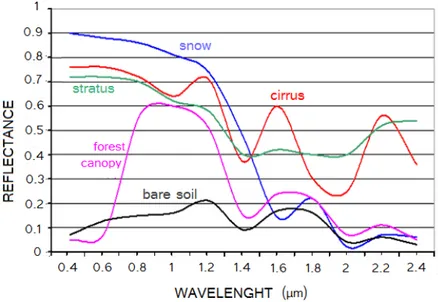
2.4 Typical reflectance values for a series of different surfaces as a function of wavelength. . . 10
3.1 (a) Scanning system of SEVIRI; (b) SEVIRI channels weighting functions. 16 3.2 AMSU-B/MHS scan geometry. . . 21
3.3 AMSU-B/MHS five channels weighting functions. . . 23
3.4 Nadir simulations of MODIS 11µm IR window channel and 6.7 µm water vapour absorption bands. . . 25
4.1 BTD test results concerning the 2006/07/03 event. . . 32
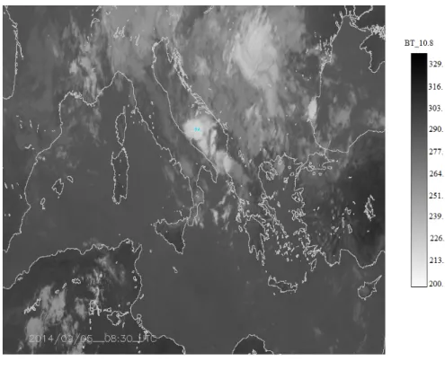
4.2 BTD test results concerning the 2014/09/05 and 2015/01/22 events. . . . 33
4.3 Schematic representation of the hail formation process. . . 34
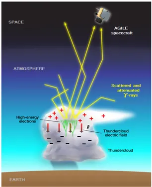
4.4 Schematic representation of Gamma-ray emission by a sever thundercloud. 35 4.5 Schematic representation of a TGF emission. . . 36
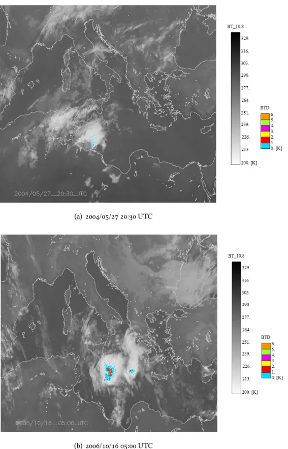
4.6 BTD test results concerning the 2004/05/27 and 2006/10/16 events with a TGF emission. . . 37
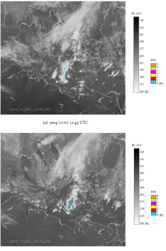
4.7 BTD test results concerning the 2004/11/07 event with a TGF emission. 38 5.1 SAFNWC CMa (a) and associated processing quality flag (b) for the 2006/10/16 event. . . 40
5.2 SAFNWC CMa remapped for the 2006/10/16 event. . . 41
5.3 Summary chart for the SAFNWC CMa remapping algoritm. . . 42
5.4 Summary chart for the SAFNWC Cloud Phase remapping algoritm. . . 44
5.5 SAFNWC CMa remapped for the 2006/10/16 event. . . 45
5.6 Summary chart for the SAFNWC CT remapping algoritm. . . 46
5.7 SAFNWC CT product for the 2006/10/16 event, before (a) and (b) after the remapping. . . 47
5.8 Summary chart for the SAFNWC CT TH remapping algoritm. . . 48
5.9 SAFNWC CT product for the 2006/10/16 event, before (a) and (b) after the remapping. . . 49
5.10 Summary chart for the MW CMa remapping algoritm. . . 50
5.11 Summary chart for the MWCC remapping algoritm. . . 51
5.12 MWCC at the satellite resolution for the 2006/10/16 event. . . 52
5.13 MW CMa (b) and MWCC (c) remapped for the 2006/10/16 event. . . 53
5.14 Analysis on the nature of misses pixels on the 2015/01/22 scene. . . 55
5.15 Analysis on the nature of misses pixels for the 2006/07/03 12:33 event. . 56
5.16 Analysis on the cloud types populating the misses category obtained by comparing the involved Cloud Masks. . . 57
List of Figures
5.17 Analysis on the cloud type populating the CMa misses category obtained
by using separately daytime and twilight/night-time scenes. . . 58
5.18 Analysis on the cloud types populating the false alarms populating the CMa misses category obtained by using separately daytime and twilight/night-time scenes. . . 60
5.19 Analysis on the cloud types populating the CMa false alarms category obtained by using separately daytime and twilight/night-time scenes. . 61
5.20 Cirrus Cloud inter-comparison. . . 63
5.21 Schematic description of the cloud type classes, in which the limits of the height ranges are underlined. . . 66
5.22 Summary of the reults obtained by applying the dichotomous statistic on the cloud type classes inter-comparison. . . 69
5.23 Very Low vs ST1 - False Alarms and Misses. . . 70
5.24 Low vs ST21 - False Alarms and Misses. . . 70
5.25 Medium vs ST3 and CO1 - False Alarms and Misses. . . 70
5.26 High vs CO2 - False Alarms and Misses. . . 71
5.27 Very High vs CO3, HSL and HSXL - False Alarms and Misses. . . 71
5.28 Summary of the reults obtained by inter-comparing, by means of the dichotomous statistic, the cloud top height SAFNWC information and the MWCC cloud classes. . . 75
5.29 Cloud top heights by SAFNWC attributed to the pixels belonging to ST1, ST2 and ST3 MWCC categories. . . 77
5.30 Cloud top heights by SAFNWC attributed to the pixels belonging to CO1, CO2 and CO3 MWCC categories. . . 78
5.31 Cloud top heights by SAFNWC attributed to the pixels belonging to HSL MWCC category. . . 79
5.32 Multilayer system outline highlighting the cloud type to which each software is responsive. . . 79
L I S T O F T A B L E S
3.1 SEVIRI channels. . . 17
3.2 PGE01 output description: Cloud Mask. . . 18
3.3 PGE02 output description: Cloud Type. . . 19
3.4 PGE02 output description: Cloud Phase. . . 20
3.5 AMSU-B/MHS instrument characteristics. . . 21
3.6 AMSU-B/MHS channels. . . 22
3.7 MWCC classes. . . 24
3.8 Contingency Matrix. . . 27
4.1 Case studies. . . 30
4.2 Case studies classified via illumination. . . 30
5.1 Cloud Mask inter-comparison results. . . 54
5.2 Numerical results deriving by the cirrus cloud inter-comparison. . . 64
5.3 Very Low vs ST1. . . 67
5.4 Low vs ST2. . . 67
5.5 Medium vs ST3 and CO1. . . 67
5.6 High vs CO2. . . 68
5.7 Very High vs CO3, HSL and HSXL. . . 68
5.8 1-2 km vs ST1. . . 72 5.9 2-4 km vs ST2. . . 73 5.10 4-5 km vs ST3. . . 73 5.11 4-6 km vs CO1. . . 73 5.12 6-10 km vs CO2. . . 74 5.13 gt 8 km vs CO3, HSL and HSXL. . . 74
1
I N T R O D U C T I O N
“Fuori s’estende la terra vuota fino all’orizzonte, s’apre il cielo dove corrono le nuvole. Nella forma che il caso e il vento danno alle nuvole l’uomo è già intento a riconoscere figure...”
– Italo Calvino,Le città invisibili
Every day looking at the sky, we get to see the wonderful sight offered by the clouds. As it appears they differ in shape, color, thickness. Some of them cause precipitation, others do not.
In addition to their enchanting and moving appearance, clouds play a very im-portant role in the mechanisms regulating life on Earth. They are an essential component of the Earth’s water cycle and global energy balance. Moreover, they are one of the most complex element in climate and atmospheric physics.
The capability to quantify with a good confidence degree the cloud cover over a region may have practical implications on the further cloud characterization (e.g. optical depth, phase, top temperature, etc.), which in turn is fundamental to derive atmospheric or surface parameters and to give insights into weather and climate processes. Different cloud types on the other hand are associated to peculiar phenomena of which clouds are tracers or precursors. Consider for example storms associated with cumulonimbus or the foehn associated with altocumulus lenticularis and rotors downwind. Thus, having a proper classification of clouds can provide a support to the forecasts of local thunderstorm activity that numerical models struggle to simulate.
Cloud detection and classification, therefore, is a very topical issue finding many applications in climate studies and operational weather forecasting. Nowadays, there are several methods which allow to perform such tasks. Visual classification methods, or in situ methods providing information on the atmospheric parameters (e.g. humidity content or local temperature), are currently used.
The methods at present most reliable are, however, those which use radiance data collected by groundbased and spaceborne sensors. For example the Radar and Light Detection and Ranging (Lidar) based on the active remote sensing technology can provide direct measurements of the vertical structure and microphysical features of clouds. They also perform an accurate atmospheric profiling with their high accuracy and an excellent space and time resolution.
INTRODUCTION
On the other hand, there are the passive remote sensing imagery and sounders, which have become perhaps the main tool for the cloudy scenario analysis. They investigate the underlying atmosphere from space, thus acquiring information on the reflected, transmitted or emitted radiation by the underlying cloud systems. The range of wavelengths in which they work can be very broad: there are radiometers working at VIS/IR wavelengths, others in the ultraviolet, still others focusing on the microwave range. The data thus collected constitute the basis for the totality of operational algorithms for cloud detection and classification.
In this work the output data obtained via two methods with very different charac-teristics will be examined and compared. One of them will be selected among the tools exploiting the VIS/IR data acquired by the geostationary satellite sensor SEVIRI. Specifically we will deal with the Cloud Mask (CMa), Cloud Type (CT), and Cloud Top Temperature/Height (CT TH) produced by the SAFNWC software package. This kind of technology was already used by more than half a century and is especially suitable for retrieval and classification of cloud properties. Actually, clouds present a significant reflectivity at visible wavelengths if compared to that of most other surfaces and emit thermal energy in the infrared region. Thus, spatial differentiation and thresholding techniques exploiting this kind of electromagnetic radiation can be used in order to detect and classify the cloud cover.
The second method used in the comparison will be a novel algorithm named MWCC. This techinque is able to reveal the vertical development of clouds while providing useful information on cloud type and cloud top height. Generally, the MW observations are very useful to provide information on the Earth’s atmosphere, due to their penetration of the clouds with respect to VIS/IR measurements. In fact, if the optical frequencies only provide a measure of radiation from the top of clouds, microwave radiation can propagate through clouds showing a better ability to sense the bulk of cloud droplets interacting with radiation field and the underlying surfaces. For this reason, microwaves show high potentialities in detecting liquid water and ice content into the clouds by enhancing the possibility to retrieve the amount of rain for their direct link with the extinguished radiation by hydrometeors.
Thus, as will be more thoroughly explained throughout the following chapters, the microwave radiation generally is not employed to detect or classify the cloudy scenarios. In the last few years, however, some focused studies revealed the potential of certain MW channels employement in order to obtain a characterization of the structure of the thunderstorm convective core. The MWCC represents one of the earliest examples.
The purpose of the present effort is an evaluation the MWCC performances with respect to the SAFNWC products. Since they are totally different from a physical point of view, it results quite interesting to quantitatively evaluate their convergences and divergences, by also investigating the technical and scientific causes. Therefore, an inter-comaprison among the output they produce will be carried out. In a first stage their power of cloud detection will be tested so as to determine whether the different technologies produce the same results in identifying cloud presence or absence. Subsequently, over the regions covered by cloud according to both
INTRODUCTION
softwares, a study will be performed in order to assess the agreement extent in the cloud classification. This work may also be useful in order to test the MWCC algorithm which still has not any kind of official numerical validation. Important information for its future development can thus be derived.
2
O V E R V I E W O F C L O U D D E T E C T I O N A N D C L A S S I F I C A T I O N M E T H O D S
The detection and the classification of clouds has always had a number of important applications in weather and climate studies. However, the scientific investigation of clouds dates from the early nineteenth century, when the French naturalist Jean Baptiste Lamarck and the Englishman chemist Luke Howard indipendently proposed the first visual methods for cloud classification. Lamarck’s work was soon forgotten, whereas the Howard’s activity was much more successful. He applied the Linnean principles of natural history for a visual cloud categorization, by using the universal Latin for the nomenclature and by also emphasizing the mutability of cloud systems [Howard (1803)]. The four basic cloud categories he introduced were: Stratus or predominantly horizontally rather than vertically extended clouds;Cumulus or cloud further extending in height;Cirrus or filamentous white clouds, that he described as “parallel, flexuous, or diverging fibres, extensible in any or all directions”. He combined these names to form four more cloud types, among which there was the Nimbus category, or the precipitating one1
.
A long time has elapsed since then, but such a scheme of distinguishing and grouping clouds perfected through the years by a large number of scientists, is the one still adopted by the World Meteorological Organization (WMO) and published in the International Cloud Atlas (1956). WMO currently recognizes 10 cloud main genera, which describe where in the sky they form and their approximate appearance: • Low clouds: lying between 0 and 2000 m, among which there are Cumulus,
Nimbostratus, Stratus and Stratocumulus;
• Middle clouds: ranging in 2000 and 7000 m, they include Altocumulus and Altostratus;
• High clouds: to which Cirrus, Cirrostratus and Cirrocumulus belong;
• Vertically developed clouds affecting more layers and essentially including the toweringCumulonimbus.
This classification scheme is summarized in figure 2.1. Moreover, these genera are further subjected to a secondary classification on the basis of shape and internal struc-ture, and also to a tertiary one, describing the cloud transparency and arrangement. In all there are about 100 combinations.
Over the last two centuries, the cloud cover quantification and qualification performed via a visual analysis, has remained in use. An example is represented by
1 taken from http://www.rmets.org/weather-and- climate/observing/ luke- howard-and- cloud- names.
OVERVIEW OF CLOUD DETECTION AND CLASSIFICATION METHODS
Figure 2.1: WMO official classification of the 10 main cloud genera.
the system mostly employed in aviation in order to assess the cloud cover amount. By using a convex mirror, it assimilates the overhanging portion of the sky to a circle to be divided into eight segments calledoktas. Subsequently, according to the oktas fraction covered by cloud, the cloudy, half-cloudy, clear or the intermediate statuses are assigned2.
Nevertheless, the cloud detection and classification methods have greatly grown up with technology advances. In particular, the real change in this research field was the beginning of the remote sensing, bothactive and passive:
• Active sensors transmit a pulse of electromagnetic energy to monitor the earth surface and atmosphere components. This is directed toward the target and once reflected off it returns to sensors thus providing a wide range of information. Examples of active sensor are Radar and Lidar.
• Passive sensors measure the reflected solar and the emitted radiation from the earth-atmosphere system. Equipped with spectrometers they measure signals at several spectral bands simultaneously, resulting in so-called multispectral images which allow numerous interpretations.
Remote sensing in the modern sense of the term begins after the World War II, when 25 airborne radars modified for ground meteorological use entered the forecasting practice. Just at the same time a large importance was acquired by the global scale observations and especially by the radiosounding network, which
2 more info e.g. available onhttp://www.metoffice.gov.uk/media/pdf/k/5/Fact_sheet_No._17.pdf
andhttps://bmtc.moodle.com.au/mod/book/view.php?id=2171&chapterid=36
OVERVIEW OF CLOUD DETECTION AND CLASSIFICATION METHODS
allowed a constant monitoring of the planetary situation up to 15-20 km height. Also the airborne observations became determinants in this field, starting to carry instruments suitable for meteorological studies.
Anyway, the greatest innovation in the remote sensing field came with the launch of meteorological satellites. These could cover much more land surface than planes and also monitor areas on a regular basis. The ability to derive an accurate cloud mask from satellite data under a variety of conditions has thus been a research topic since launch of the the first satellite bringing on board meteorological instruments, or the Vanguard-2 in 1959. Designed by the National Aeronautics and Space Administration (NASA), this mission was conceived to measure cloud cover distribution over the daylight portion of its orbit3. However, due to an unsatisfactory orientation of the spin axis the telemetry data resulted to be poor and then, the first images actually transmitted by a weather satellite, date back to year 1960, when NASA sends into orbit Television and Infrared Observation Satellite Program (TIROS) - 1. It was equipped with two vidicon cameras, at the time typically used for the television broadcast, and remained operational for 78 days4.
Since then, several geostationary and polar-orbiting meteorological satellites were launched and the constantly developing technology of the onboard instruments allowed to acquire information pertaining to a wide electromagnetic frequency range from the ultraviolet (UV), to visible (VIS), near-infrared (NIR), infrared (IR) and MW wavelenghts. The main energy source for the earth-atmosphere system is represented by solar radiation, travelling as an electromagnetic wave extending all over electromagnetic spectrum, from the UV to IR. The incoming solar radia-tion is partly absorbed, partly deflected (orscattered) and partly reflected by the atmospheric gases, aerosols and clouds (figure 2.2). The remaining energy fraction reaching surface is almost completely absorbed and only partly reflected. After that, the absorbed radiation is re-emitted towards space at different wavelenghts. As this happens, clouds and other atmospheric gases interact again with the incident radiation and coming from various directions, further reflecting, absorbing and then emitting, or scattering. A discussion of the heat balance of the atmosphere can be found inWallace and Hobbs (1979).
The solar radiation reaches its maximum in the visible (short wave radiation), whereas the earth emitted radiation has its peak in the thermal IR (long wave radiation) as illustrated in figure 2.3. The first sensors built and put side by side to the vidicon cameras were able to work in the visible frequencies and to acquire radiances reflected from the underlying surfaces. Actually clouds have a high solar reflectivity in the visible compared to that of most surface features as shown in figure 2.4. Thus, spatial differentiation and thresholding techniques could be used to distinguish clouds from less reflective land and ocean surfaces. Then to the simple visible sensors the infrared channels were added in order to characterize the cloud coverage on the basis of cloud emitted radiation. IR brightness temperatures can
3 http://nssdc.gsfc.nasa.gov/nmc/spacecraftDisplay.do?id=1959- 001A. 4 http://science.nasa.gov/missions/tiros/.
OVERVIEW OF CLOUD DETECTION AND CLASSIFICATION METHODS
Figure 2.2: Radiative balance of the Earth: the incoming solar radiation is partly absorbed, partly scattered and partly reflected by the atmospheric gases, aerosols, clouds and Earth surface. A fraction of the absorbed radiation is re-emitted in the thermal bands. Note that the percentages of each kind of radiation are shown too. Image available online at http://www.thermopedia.com/content/569/ #ATMOSPHERE_FIG2.
be used as a proxy for the surface or cloud top temperatures, which under normal lapse rate conditions, decrease with height. Therefore when the emitted radiance is converted to equivalent blackbody temperature it can be used to distinguish the presence of opaque clouds from a warm surface.
For example, the National Oceanic and Atmospheric Administration (NOAA) Scanning Radiometer (SR), put into operation in 1970, measured reflected radiation from the earth-atmosphere system in the 0.52 - 0.73µm (VIS) band during the day and the emitted radiation in the 10.5 - 12.5µm (IR) band during the day and night5. It was put side by side with vidicon cameras, but unlike a camera, it formed an image by using a continuously rotating mirror which acquired radiances coming from below.Rossow et al. (1983) used the SR imagery in order to derive the cloud amount, optical thickness and cloud top temperature in a pilot programme aimed to develop a cloud climatology.
The SR successor was the Advanced Very High Resolution Radiometer (AVHRR)/2 aboard the NOAA polar orbiting satellites. It gave daily global coverage in 5 spectral bands ranging from 0.58 - 12.5µm (the latest and improved instrument version, AVHRR/3, is still operating and is equipped with 6 spectral channels). Several attempts were made over the years in order to establish AVHRR data processing
5 http://nssdc.gsfc.nasa.gov/nmc/experimentDisplay.do?id=1970- 106A-03.
OVERVIEW OF CLOUD DETECTION AND CLASSIFICATION METHODS
Figure 2.3: Solar and Earth black body radiation emission curves. In the lower panel also the instrumentation sensitivity to the different kind of radiation is highlighted. Taken fromMenzel (2012).
schemes able to provide an accurate cloud cover estimation and sometimes also a cloud type analysis [e.g Liljas (1984) or Arking and Childs (1985)]. Some of these techniques for example considered the spatial variance of infrared radiances to separate the clear or cloudy scenes [Coakley and Bretherton (1982)]. However, the first algorithm making use of all 5 the AVHRR spectral channels was AVHRR Processing scheme over cLouds, Land and Oceans (APOLLO). After deriving some physical properties, it processed each pixel of the imagery, to which a label was assigned according to whether its radiance was lower or higher than the given threshold.
In other words, the first stage of the APOLLO software processing scheme is to generate a cloud mask product via a set of threshold tests, distinguishing four categories (cloud free, fully cloudy, partially cloudy, and snow/ice) [Saunders and Kriebel (1988)]. Subsequently the cloud cover is derived for each fully cloudy or partially cloudy pixel, according to two different methodologies. In particular each fully cloudy pixel is checked for the presence of thin or thick cloud, based on the VIS relectances during the day and on the IR brightness temperatures during night-time [Kriebel et al. (1989)]. Pixels covered by thick clouds are considered water cloud filled, whereas thin clouds are treated as ice clouds, i.e. cirrus. In case of partially cloudy pixels the cloud coverage is obtained through the reflectances and temperatures of the cloudy and cloud-free portion of the pixels. These quantities are taken from the nearest fully cloudy and cloud-free pixels, assuming horizontal homogeneity. The cloud cover of the partially cloudy pixels is assigned to the most frequent cloud type in a 50 by 50 pixels environment. Finally cloud optical depth, liquid/ice water path and emissivity are derived during daytime for every fully cloudy pixels by means of parameterization schemes based on the VIS reflectance, whereas the cloud top
OVERVIEW OF CLOUD DETECTION AND CLASSIFICATION METHODS
Figure 2.4: Typical reflectance values for a series of different surfaces as a function of wavelength, taken fromJedlovec (2009).
temperature is obtained by means of a correction for the water vapour above the cloud [Kriebel et al. (2003)].
Later on, other operational algorithms partly referred to APOLLO were developed [e.g. Stowe et al. (1991), Derrien (1993)]. An example was an automated cloud classification model based on NOAA/AVHRR satellite data, named SMHI Cloud ANalysis model using DIgital AVHRR data (SCANDIA). The SCANDIA first version was implemented in 1988 [Karlsson (1989)] and it operated exclusively on Sweden and adjacent areas. SCANDIA made use of imagery from all 5 AVHRR/2 channels at maximum horizontal resolution (at nadir 1.1 km) and it was based on a series of threshold tests performed on the acquired brightness temperatures or reflectances differences [Karlsson and Liljas (1990)].
However these methodologies based on the exploitation of the AVHRR polar sensors did not ensure the adequate space-time coverage requested for a regular monitoring of the cloudy scenarios. This could be provided by continuos framing of the geostationary satellites, able to observe a large portion of Earth surface. So, the first of the Geostationary Operational Environmental Satellites (GOES), was launched in October 1975. Two more followed, in June 1977 and 1978 respectively. Such satellites were spin stabilized spacecraft, which provided imagery through the Visible Infrared Spin-Scan Radiometer (VISSR). The instrument, by using a common optical system, acquired information both in a VIS and an IR spectral band6. Besides in November 1977, the first among the geostationary meteorological satellites of the Meteosat programme was launched too. It provided Earth and atmosphere images every half-hour in three spectral channels via the Meteosat Visible and Infrared Imager (MVIRI) instrument. In addition to acquiring information in the VIS/IR range, this is one of the very first cases in which a channel centered in an IR water vapour
6 http://nssdc.gsfc.nasa.gov/nmc/experimentDisplay.do?id=1977- 048A-01.
OVERVIEW OF CLOUD DETECTION AND CLASSIFICATION METHODS
absorption band was used. It was more sensitive to the water vapour variations furthemore providing important data about the water vapour amount.
After that, a series of new automatic methods for cloud detection and classification using the operational analysis of geostationary satellite data, were thus developed. In literature, in addition to thethreshold techniques [Minnis and Harrison (1984); Rossow et al. (1985)] also some statistical methods appeared. These classified a pixel as belonging to a specific cloud class, by costructing frequency histograms considering the image as a whole and then evaluating the position of such pixel in the feature space [Desbois et al. (1982); Simmer et al. (1982); Porcù and Levizzani (1992)].
These experiments clearly surfaced the need for an increasing number of spectral channels. Many authors pointed out that such additional information could improve the cloud detection and differentiation quality [e.g. Desbois et al. (1982); Coakley (1983)]. Some of them have especially focused on the high-altitude cirrus cloud distinction, wich in general resulted quite difficult owing to contamination of the IR frequency signal by the underlying layers (lower clouds or surface) [Inoue (1985); Jin and Rossow (1997)].
The last twenty years have seen great progresses in this direction. The latest technology, in fact, allowed to increase the multispectral capabilities of the new generation of VIS/IR imager. Among them, in addition to improved version of the instruments belonging to the previous releases (e.g. AVHRR and GOES), the Moderate Resolution Imaging Spectroradiometer (MODIS) must be mentioned. The instrument was launched into Earth orbit by NASA on board theTerra (1999) and Aqua (2002) satellites belonging to the Earth Observing System (EOS)7
programme. The instruments make measurements in 36 spectral bands ranging in wavelength from 0.4 to 14.4µm and at varying spatial resolutions (250, 500 and 1 m). They are designed to provide measurements of large-scale global dynamics including changes in Earth’s cloud cover, radiation budget and processes occurring in the oceans, land and lower troposphere [Ackerman et al. (1998); Frey et al. (2008)]. The MODIS operational cloud products consist of cloud mask, cloud top properties (i.e. temperature, pressure, effective emissivity), cloud thermodynamic phase, cloud optical thickness and microphysical properties. The cloud mask algorithm identifies several conceptual domains according to the kind of surface and solar illumination. After that a series of threshold tests attempt to detect the presence of clouds, returning also a confidence level that the pixel is clear, ranging in value from one (high confidence clear) to zero (low confidence clear). The four confidence levels thus included in the output are: confident clear, probably clear, uncertain/probably cloudy and not clear/cloudy [Platnick et al. (2003)].
A turning point was also constituted by the Meteosat Second Generation (MSG) geostationary satellites carrying on board the SEVIRI. With its 12 spectral channels and a high spatial and temporal resolution, the observations thus provided have shown large improvements in the cloud property retrieval. The data thus collected are now processed through a wide variety operational tools, including the most
OVERVIEW OF CLOUD DETECTION AND CLASSIFICATION METHODS
advanced SAFNWC software package. This topic is throughly illustrated in section 3.1.
While the VIS/IR sensors was developing, the weather satellites began to be also equipped with passive MW sensors.
Electromagnetic radiation in the reange of microwave wavelenghts is charac-terized by a mechanism of interaction with matter different than other spectral regions. Microwave radiation emission from an object is strongly tied to the physical properties of the object itself, such as atomic composition and crystalline structure. Contrarily to the IR spectral region where the black body approximation often well describes the real behaviour of the emitters, the microwave emitters surfaces must be considered as a grey body with an emissivity value typically lower than 1.
The great advantage of these frequencies with respect to the optical ones is the high capability to penetrate the majority of clouds [e.g.,Greenwald and Cristopher (2002);Burns et al. (1997)]. Moreover, contrarily to VIS/IR observations, which only sense reflected or emitted radiation from the cloud top, microwave radiation can propagate through clouds, showing sensitivity to the total cloud layer in addition to the potential to estimate cloud water and ice contents (see section 3.2).
For this reason, since the introduction of the first radiometers able to capture this kind of long wave radiation, the data acquired were not used for cloud detection or classification, but rather to obtain information about the water vapour atmospheric column or about the underlying surfaces.
For example, spaceborne MW observation were obtained by the the Special Sensor Microwave/Imager (SSM/I), a 7 channels, four-frequency, linearly polarized passive microwave radiometer system on board the Defense Meteorological Satellite Pro-gram (DMSP) satellite. It measured surface and atmospheric microwave brightness temperatures at 19.35, 22.235, 37.0 and 85.5 GHz and it has been a very successful instrument. Its combination of constant-angle rotary-scanning and total power ra-diometer design has become standard for passive microwave imagers, e.g. Advanced Microwave Scanning Radiometer (AMSR). Over ocean, cloud liquid water paths were routinely estimated from the cloud emissions measured between 19 and 85 GHz by such a kind of imagers [e.g.Greenwald et al. (1993); Ferraro et al. (1996); ODell et al. (2008)]. Moreover, due to the strong contamination of the surface type (different emissivity) on microwaves measurements, over land the problem was more com-plicated. The land surface emissivity generally ranges between 0.6 and 1, making atmospheric features difficult to identify against such a background because of the limited contrast. In addition, the land surface emissivity is variable in space and time and difficult to model. Efforts have been made to estimate cloud liquid water over land, using a priori information on the surface properties [Aires et al. (2001)].
At frequencies below 80 GHz, the microwave signal is essentially dominated by emission and absorption by cloud droplets and rain and is little affected by the presence of ice. At higher frequencies, the scattering effect on frozen particles increases. Ice particles modify the upwelling radiation by scattering photons away from the satellite sensors, causing a brightness temperature depression. Then, from
OVERVIEW OF CLOUD DETECTION AND CLASSIFICATION METHODS
observations above 80 GHz, cloud ice information has been extracted from both imagers such as SSM/I and water vapour sounders such as the AMSU-B, a passive microwave sounder on board the NOAA polar orbiting satellites, operationally used to estimate temperature and water vapour atmospheric profiles [Greenwald and Cristopher (2002); Hong et al. (2005a); Weng et al. (2003)], as will be throughly explained in section 3.2.
Therefore, the physical properties of microwaves have been fully exploited in the weather analysis, albeit only in recent years they begun to be employed for detecting or classifying clouds. A criterion based on the difference between measured brightness temperatures at the three AMSU-B channels centered in the MW water vapour absorption band (183.31 GHz) was suggested in order to screen out convective clouds by Burns et al. (1997). The same channels have also been used for the production of information about the convective core of the tropical cyclons [Hong et al. (2005a)].
In 2011,Aires et al. tried a statistical cloud classification and cloud mask algorithm on the basis of AMSU-B observations, by using the VIS/IR data from SEVIRI in order to train the microwave classifier. They obtained in this way a confidence level of more than 80%,
In the last few years, a multichannel passive microwave cloud classification algo-rithm has been developed in the context of the rain rate retrieval algoalgo-rithm Water vapour Strong Lines at 183 GHz (183-WSL) [Laviola and Levizzani (2011); Laviola et al. (2013)]. It is able to detect and also to classify the mid-latitude clouds and also to give important information about the deep convection vertical development, by using the brightness temperatures of the three MW water vapour opaque channels (see subsection 3.2.2).
In the present work we propose to understand differences and errors that may take place by using two indipendent methods for cloud detection and classification based on different physical features. One of them will be chosen among the VIS/IR-based software packages, the other one instead will be an algorithm working in the MW frequencies. Although both, in principle, are intended to provide the same kind of output, as based on different physical principles they should sometimes “see” different cloud properties. What we intend to do, is to quantitatively evaluate their deviation, trying to explain the technical and phenomenological causes.
3
T O O L S A N D M E T H O D S
The basic purpose of this research work, as already discussed in the previous chapters, is to assess the differences between two methods for cloud detection and cloudy scenario classification. The two methods are based on satellite data from different parts of the electromagnetic spectrum, one in the MW and the other in the VIS/IR wavelengths. What we intend to do, is to quantitatively evaluate their differences and to explain the technical and phenomenological causes.
Thus, the first part of this chapter describes the characteristics of the two classi-fication algorithms, by focusing on their different scientific basis, the output they produce, and the satellite sensors whose data are used as input.
Whereupon, a threshold test based on the brightness temperature difference (BTD) between SEVIRI data acquired in the water vapour absorption band centered at 6.2 µm and in the IR atmospheric window at 10.8 µm (i.e. where atmospheric absorption/emission is negligible) is illustrated. It will be employed in the following analysis as a first investigation method in order to verify the severity and vertical extent of each analysed cloud system.
Afterwards, a brief description of dichotomous statistics will follow, used as a tool for the quantification of the differences between the two cloud classification algorithms.
3.1 v i s / i r d ata a c qu i s i t i o n a n d p r o c e s s i n g
This section illustrates the characteristics of the SEVIRI instrument on board the MSG satellites and the SAFNWC software package. This latter together with SEVIRI data are exploited in this study for the cloudy scenario analysis in the VIS/IR spectral range.
3.1.1 SEVIRI instrument
The MSG consists of a series of four geostationary satellites in a circular orbit at about 36000 km above the equator with the same Earth’s angular rotation speed. The monitoring service is currently provided by MSG-3, the prime operational geostationary satellite positioned at0 degrees and providing full disc imagery every 15 minutes. MSG-2 is exploited for the Rapid Scanning Service, delivering more frequent images every five minutes over parts of Europe, Africa and adjacent seas, whereas MSG-1 presently serves as back-up to both sensors. The last satellite of the MSG series, MSG-4, was launched on July 2015. The current policy is to keep two
TOOLS AND METHODS
(a) (b)
Figure 3.1: (a) Scanning system of SEVIRI; (b) Weighting functions for SEVIRI channels 4-11 (from http://eumetrain.org/data/2/204/204.pdf ).
operational satellites in orbit and to launch a new satellite close to the date when the fuel on the oldest of the two starts to run out1.
The main MSG payload is SEVIRI, a 12-channel imager observing the earth-atmosphere system. It provides detailed information due to an imaging-repeat cycle of 15 minutes and image sampling distance of 3 km at nadir for all channels, except the high-resolution visible (HRV) at 1 km. For the first 11 channels a full SEVIRI image consists of 3712×3712 pixels and is acquired in about 12 minutes by combining satellite spin and rotation of the scan mirror. This phase is followed by a brief calibration of the thermal infrared channels, after which the scanning mirror returns to its initial position, by obtaining in this way the repeat cycle of 15 minutes [Schmetz et al. (2002)]. Such acquisition mechanism proceeds from east to west and from south to north, as shown in figure 3.1(a).
The 12 channels of SEVIRI are centred at frequencies covering the portion of electromagnetic spectrum ranging from visible to infrared. The weighting functions displayed in figure 3.1(b) and the spectral channels illustrated in table 3.1, demon-strate that each channel has been selected in order to gather information on the major atmospheric constituents, the earth’s surface and the cloud cover.
3.1.2 SAFNWC software package
The software package developed by SAFNWC includes 12 Product Generator Ele-ments (PGEs), i.e. softwares for the retrieval of variuos cloud analysis products from SEVIRI data. The PGEs can generate products over a user-defined area within the full disk, thus providing useful information for nowcasting applications.
For the data analysis carried out in the following, only three PGEs have been used, i.e. PGE01 providing the Cloud Mask (CMa) product, PGE02 for the Cloud
1 more info available on https://directory.eoportal.org/web/eoportal/satellite- missions/m/ meteosat- second-generation.
3.1 v i s / i r d ata a c qu i s i t i o n a n d p r o c e s s i n g
Table 3.1: SEVIRI channels.
Type (CT) and Cloud Phase extraction, and, finally the PGE03 generating the Cloud Top Temperature/Height (CT TH) information.
The first two products provide, respectively, a cloud detection and classification and are performed via a multispectral thresholding technique [Derrien and Le Gléau (2005)]. With regard to the computation of cloud top height, instead, the technique depends on the cloud type as available in the CT product [Derrien (2013)]. For exam-ple in case of opaque clouds, the CT TH values can be deduced from the brightness temperature (BT) acquired in the IR window channels. This technique cannot be applied in presence of semitransparent or fractional clouds, mainly due to contam-ination of the BTs in the IR frequencies by the underlying surface. Therefore, a multispectral approach is needed.
The software works also in case only a limited number of channels are available. Actually, even if the optional information enables to perform a more accurate analysis, the CMa and CT algorithms mandatory input are the BTs acquired at 3.9, 10.8 and 12.0µm, in addition to the radiance at 0.6 µm. The CTTH module needs the IR10.8 channel information and at least one among the 6.2, 7.3 and 13.4µm radiances.
Most thresholds and coefficients are computed from ancillary data and radiative transfer models, by obtaining in this way values specifically computed for any
TOOLS AND METHODS
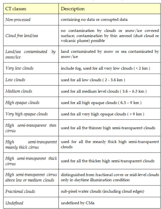
Table 3.2: PGE01 output description: Cloud Mask.
time and geographical area selected by the user. Ancillary data mainly consists of atlas, climatology maps and Numerical Weather Prediction (NWP) model forecast fields, supplied by European Centre for Medium-Range Weather Forecasts (ECMWF) on specific user request. The Second Simulation of a Satellite Signal in the Solar Spectrum (6S) advanced code [Tanre et al. (1990); Kotchenova et al. (2006)] is exploited to simulate the atmospheric effects in the solar bands and for the pre-computation of a great variety of parameters (e.g., angles, water vapour and ozone content).
On the other hand, among the fast radiative transfer model employed there is also the Rapid Transmissions for TOVs (RT TOV) [Eyre (1991); Saunders et al. (1999)]. It works in the thermal bands and is applied to radio-soundings from a data set provided by ECMWF [Chevallier (1999)] in order to compute the look-up tables subsequently used for the threshold calculations. In the CT TH module context, the RT TOV is also applied using NWP temperature and humidity vertical profile to simulate 6.2, 7.3, 10.8, 12.0 and 13.4µm cloud free and overcast radiances and brightness temperatures2. This process is performed online on each segment of the processed image.
The overall operational strategy of the SAFNWC software package involves, as a first step, the detection of clouds by the CMa software. It delineates all absolutely cloud free pixels in a satellite scene with a high degree of confidence and identifies pixels that are contaminated by either clouds, dust or snow/sea ice. Whereupon, each pixel classified as cloudy is distinguished per type using the CT module, which is also able to produce a further output concerning the cloud particle phase (CT_PHASE). Only after these two steps, the application of the third module, CT TH, provides information about cloud top temperature or, in an equivalent way, height or pressure.
2 sourcehttp://www.nwcsaf.org/HD/MainNS.jsp.
3.1 v i s / i r d ata a c qu i s i t i o n a n d p r o c e s s i n g
Table 3.3: PGE02 output description: Cloud Type.
Finally, on all the mentioned products a parallax correction is applied by means of a dedicated tool included in the software package.
The output content of PGE01 and PGE02 (both cloud type and cloud particles phase) is illustrated in tables 3.2, 3.3 and 3.4, respectively3.
In table 3.3 it can be observed that, by using PGE02, it is also possible to make a distinction between high semi-transparent (cirrus) clouds and high or very high opaque clouds. Moreover, for medium to low and high opaque cloud classes, a rough
TOOLS AND METHODS
Table 3.4: PGE02 output description: Cloud Phase.
evaluation of the range of clouds top heights, obtained by analysing statistics of retrieved cloud top pressure, is provided [Derrien (2013)].
A quality flag is associated to each products, describing, among other things, illumination conditions and quality of the processing itself.
As regards the illumination parameter we can distinguish: night-time (solar ele-vation <-3°),twilight (-3°< solar elevation <10°), daytime (10°< solar elevation) and sunglint (Re fCox>10%4, solar elevation >15°) .
On the other hand, the quality flag provides an indication of the confidence attributable to the retrieval processes and its possible values are:
0 Non-processed: containing no data or corrupted data;
1 Good quality: high confidence;
2 Poor quality: low confidence;
3 Reclassified: (after spatial smoothing) very low confidence5.
For CMa and CT products a pixel is flagged as of low confidence if for each executed test the difference between the threshold value and the mesurements is lower than a specified tolerance value depeding on the test itself. In the CT TH retrieval, however, the quality assessment is conditioned by the cloud type and the used retrieval techniques [more info are available inDerrien (2013)].
3.2 m w d ata a c qu i s i t i o n a n d p r o c e s s i n g
This section contains technical and physical information on the AMSU-B/MHS radiometers and on the MWCC algorithm, respectively used for data acquisition and processing in the MW frequencies for cloud type characterization.
4 Re fCoxstands for the top of atmosphere reflectance at 0.6µm simulated over the ocean using the Cox and Munck theory [Cox and Munck (1954)].
5 flag number3 is available only for CMa and CT products, not for CTTH.
3.2 m w d ata a c qu i s i t i o n a n d p r o c e s s i n g
3.2.1 AMSU-B/MHS instrument
The AMSU-B is a five-channel microwave radiometer, whose main purpose is the retrieval of global data on water vapour profiles. It works combined with the fifteen-channel AMSU-A, to provide a 20 fifteen-channel microwave radiometer. Both sensors are installed on board the Meteorological Operational satellite programme (MetOp) and NOAA - K, L, M polar-orbiting satellite series flying in sun-synchronous orbit. For NOAA-18 (NOAA - N) satellite, AMSU-B was replaced by the new generation radiometer MHS with basically similar characteristics of its predecessor.
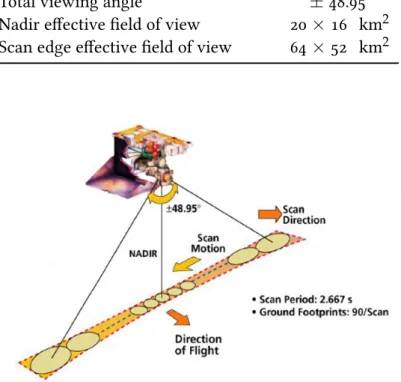
The AMSU-B/MHS instrument is cross-track scanning, so it acquires continuously scene radiances at each channel frequency in awhisk broom mode, as illustrated in figure 3.2. During each 8-second observation cycle, it makes 3 scans of 90 observa-tions each, with a spacing of 1.1° [NOAA(2009)]. Further information on the spatial resolution of the instrument is given in table 3.5 [Saunders et al. (1995); Bennartz et al. (2002)].
Table 3.5: AMSU-B/MHS instrument characteristics.
Spatial resolution 1.1° Total viewing angle ±48.95° Nadir effective field of view 20×16 km2 Scan edge effective field of view 64×52 km2
Figure 3.2: AMSU-B/MHS scan geometry.
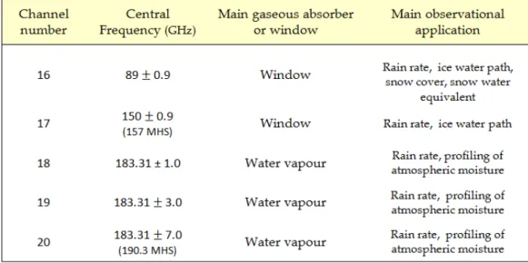
The instrument works within a wide frequency range, from 89 to 190 GHz: two of its channels are nominally centred in the atmospheric window frequencies 89 and 150 GHz, whereas the other three are selected within the water vapour absorption band at 183.31 GHz (see table 3.6) and hereafter defined as the 184, 186 and 190 GHz channels.
TOOLS AND METHODS
Table 3.6: AMSU-B/MHS channels.
The two window channels, 16 and 17, as such, can sense through the lower atmosphere, as can also be observed by looking at the respective weighting functions peaks, shown in figure 3.3. According toHong et al. (2005b), even in the case of deep convection the surface emissivity greatly influences the channel at 89 GHz and, even if to a lesser extent, that at 150 GHz . This ability to see the lower layers makes them greatly affected by the kind of background and, thus, not very useful in precipitation retrieval or in medium-high cloud observations.
The other three channels, instead, being selected in a water vapour absorption band, were originally designed and dedicated to the profiling of the atmospheric moisture [Wang and Chang (1990); Wilheit (1990)]. However, several studies on the effects of clouds on microwave radiances at the AMSU-B/MHS channels, performed through observations [e.g.,Wang et al. (1997); Hong et al. (2005b)] and simulations [e.g., Muller et al. (1994); Burns et al. (1997); Bennartz and Bauer (2003)], have demonstrated that these three channels are very sensitive to ice crystals and rain drops. So, the combination of scattering by the former and absorption by the latter, largely contribute to radiation extinction.
On the other hand, due to their weighting functions peaking between 2 and 8 km altitude (figure 3.3), low level-clouds and surface emissivity have little effects on the signal detected within these wavelengths [Hong et al. (2005b)]. This means having at the same time the advantage of probing successfully over any surfaces, but also the disadvantage while observing clouds lying within lower atmospheric layers, which are virtually undetectable.
Moreover for such opaque channels, in the presence of hydrometeors in the upper level of vertically developed clouds, the farther is the frequency from the centre of the water vapour absorbtion band, the larger is the brightness temperature depression [Burns et al. (1997)]. In other words, the 190 GHz frequency displays the greatest signal extintion, followed by the 186 and 184 GHz. This happens because their
3.2 m w d ata a c qu i s i t i o n a n d p r o c e s s i n g
Figure 3.3: AMSU-B/MHS five channels weighting functions. The peaks heights, described in the above figure, change critically in the presence of a cloud system or of a great amount of water vapour.
weighting functions reach their maximum at different altitudes, and the more distant channel (190 GHz) can see deeper through clouds than the others, as illustrated in figure 3.3.
From sensitivity studies byHong et al. (2005b) for deep convection in the Tropics, it appears also that the 190 GHz channel, as well as being the one that can see deeper inside the convective core, is also the one that has the strongest sensitivity to the frozen hydrometeor scattering and the channel within which there is the strongest incident radiation absorbtion by water vapour inside or surrounding clouds.
Therefore, for the 183.31 GHz AMSU-B/MHS channels, the magnitude of signal extinction depends both on the height of the scattering hydrometeors and on the channel wavelengths.
3.2.2 MWCC algorithm
All the physical features outlined in subsection 3.2.1, suggest the potential to delineate a vertical structure of deep convective systems by using the three water vapour channels centred at 183.31 GHz, as already shown byHong et al. (2005a) in their analysis on the tropical systems.
Along the same lines as the aforementioned work, a new method has been stud-ied to detect and classify the mid-latitude clouds and to give more information about the cloud vertical development, by using the brightness temperatures of these three opaque channels. Such method for the MicroWave Cloud-type Classifica-tion (MWCC) has been developed in the context of the rain rate retrieval algorithm
TOOLS AND METHODS
183-WSL [Laviola and Levizzani (2011); Laviola et al. (2013)], acquiring, subsequently, an its own identity while still being finalized.
It works by calculating the differences between the brightness temperature ob-served on a clear sky pixel and brightness temperatures recorded in the three 183 GHz frequencies. Thus on the basis of the signal perturbations, it performs a series of threshold tests selected by means of statistical analysis on several events particularly occurring in mid-latitudes.
Through the use of the MWCC, it is possible to detect the presence of clouds and to evaluate a cloud type in terms of stratiform (ST) and convective (CO) clouds by identifying three intensity classes for each type and evaluating the cloud top height.
As illustrated in table 3.7, to each class a range of heights is associated: in some cases this definition bands are rather wide and in some others these are overlapped. All of this is due to the principle on which the algorithm works, since it assigns each class based on the height of the weighting functions peak, but, in the presence of clouds or high concentrations of water vapour, these heights vary. Therefore, the MWCC is able to give a response with respect to one atmospheric layer within which the cloud top is located, rather than an exact height value.
Table 3.7: MWCC classes in terms of cloud top height.
The algorithm has been designed in order to provide information on the vertical development of clouds in particular for convective type. Thus, starting from the identification of signal perturbation of clouds in the lower atmosphere, the MWCC method tries to identify further perturbations in the middle and higher atmosphere by assuming in a bottom-up mode the vertical continuity of cloud development. This process, if on one hand well describes stratiform and convective clouds (the continuity is guaranteed by the cloud development from the surface to the top of atmosphere) on the other is unable to represent the “isolated” clouds, such altostratus due the convection dissolution.
Recently, the computational scheme of the MWCC has been improved with a probability-based module for hail detection. It is still under revision and it aims to classify the hail by size in Hail Storm Large (HSL) and Hail Storm EXtra Large (HSXL).
3.3 b r i g h t n e s s t e m p e r at u r e d i f f e r e n c e t e s t
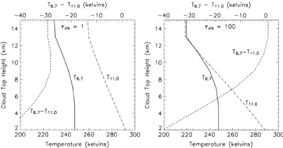
Figure 3.4: Nadir simulation of MODIS 11 µm IR window channel and 6.7 µm water vapour absorption bands for (a) optically thin and (b) optically thick clouds, illustrating their combined utility in the flagging of high-altitude, optically thick cloud structures [fromTurk and Miller (2005)].
3.3 b r i g h t n e s s t e m p e r at u r e d i f f e r e n c e t e s t
In order to identify deep convection among the cloud systems in every case studies analysed, an IR threshold test was exploited. This is based on the difference between the brightness temperatures (BTD) available in the SEVIRI channel centred in the water vapour absorption band at 6.2µm (BT6.2) and the brightness temperatures acquired in the channel residing in the infrared atmospheric window at 10.8µm (BT10.8):
BTD= BT6.2−BT10.8 (3.1) This pure infrared (and hence day/night indipendent) technique is able to detect deep convective clouds and convective overshooting, as proposed bySchmetz et al. (1997), and also to identify optically thick high altitude clouds, as suggested byTurk and Miller (2005).
With the aim of better understanding the functioning of this test, we refer to the figure 3.4. This shows some radiative transfer simulations for BT as a function of cloud top height, involving the two MODIS channels at 6.7 and 11.0µm, correspond-ing to the SEVIRI channels WV6.2 and IR10.8 respectively. Plotted in both panels are three curves depicting the variations of the BTs and their difference in two cases, for which peculiar behaviours emerge:
• Optically thin cloud (left-hand panel): the 6.7 µm signal has no sensitivity to clouds below about 5 km and the 11.0µm signal gradually decreases as the top height increases. Due to transparency of outermost layers of this cloud kind, the measured temperature does not correspond to the environmental
TOOLS AND METHODS
cloud-top temperature, but it is much higher in both bands, in this way the BTD never exceeds - 28 K for any cloud height.
• Optically thick cloud (right-hand panel): the 6.7 µm channel continues to mask the signal of low level clouds, meanwhile the 11.0µm temperature heavily decreases in accordance with the atmospheric lapse rate because of the negligi-ble cloud transmittance and near-blackbody emittance. As the cloud top rises into the upper tropospheric layers, the 6.7µm signal also begins to respond and the temperatures for both channels significantly converge, so that at the tropopause the BTD is near zero and, in the case of an increasing temperature profile in the lower stratosphere, the 6.7µm brightness temperature may actu-ally exceed that at 11.0µm due to the presence of absorbing/emitting vapour at these levels [Turk and Miller (2005)].
Therefore, according to what has been illustrated above, if an opaque cloud is strongly developed in height up to the tropopause or overshooting into the strato-sphere, the BT in the water vapour channel can approach or be larger than the BT in the infrared channel. Subsequently, the BTD that assumes values very close to zero is a useful indicator of the presence of optically thick cloud at or near the tropopause, meanwhile positive values provide a good hint on the presence of an overshooting top. Schmetz et al. (1997) found that, in these cases in contrast to the normal condition (clear sky or low level cloud), the BTD can get up to 6 - 8 K.
Thus, this simple but specific test can provide a very good information about cloud systems populating scenes to be studied in the following.
3.4 d i c h o t o m o u s s tat i s t i c s
In this work thedichotomous statistic is used to compare the outputs of both softwares described in previous sections.
The discrete dichotomous variables are nominal variables which have only two categories or levels,yes or no. In order to apply this kind of statistic to the present analysis, the response of the two different methods has to be interpreted or arranged so as to be treated like a variable, e.g. in the cloud mask case we will study the presence or absence of cloud, or cloudy(yes)/cloud free(no). Moreover, one of the analysed softwares will have to be considered as truth, then leading the comparison, (software 1) and the other to be treated as the one to be tested (software 2)6.
In this way the combination of the outputs (yes or no) of the two softwares gives rise to four event categories:
• hits: events that occur according to both softwares;
• misses: events that occur for software 1, but not for software 2; • false alarms: events that occur for software 2, but not for software 1;
6 the assignment of these two roles will be explained in chapter 5.
3.4 d i c h o t o m o u s s tat i s t i c s
• correct negatives: events that do not occur according to both softwares.
These can be represented in a 2×2 contingency matrix (table 3.8).
Table 3.8: Contingency Matrix.
A perfect agreement between the two compared systems would produce only hits and correct negatives and no misses or false alarms. Moreover, a large number of categorical statistics can be computed from the elements in the contingency matrix7. The parameters used in this study are listed below:
• accuracy (ACC), describing the fraction of correctly detected occurrences and given by
ACC= hits + correct negatives
total (3.2)
it ranges in[0, 1]and has a perfect score value equal to1;
• bias (BIAS), ranging from0 to∞, with a perfect score amounting to 1, it is defined as
BIAS= hits + false alarms
hits + misses (3.3) and it indicates whether the software 2 has a tendency to underestimate (BIAS<1) or overestimate (BIAS>1) the events;
• probability of detection (POD), defined as
POD= hits
hits + misses, (3.4) it ranges from0 to 1 with a perfect score value equal to 1, and describes what fraction of software 1 “yes” events are correctly detected by software 2;
7 more info available on the websitehttp://www.cawcr.gov.au/projects/verification/#Standard_ verification_methods
TOOLS AND METHODS
• false alarm ratio (FAR), has a perfect score amounting to0 and a value range of[0, 1], is defined as
FAR= false alarms
hits + false alarms (3.5) and indicates the fraction of detected events by software 2, which do not occurr according to software 1;
• probability of false detection (POFD), which represents the fraction of the software 1 “no” events that are incorrectly classified as “yes” by software 2, is given by
POFD= false alarms
correct negatives + false alarms (3.6) with a perfect score amounting to0 in the range of values[0, 1];
• Heidke Skill Score (HSS), even known as theCohen’s κ, is defined as
HSS = (hits+correct negatives) − (expected correct)random
total− (expected correct)random (3.7)
where
(expected correct)random = 1
total[(hits+misses)(hits+false alarms)+ (3.8)
+ (correct negatives+misses)(correct negatives+false alarms)].
The HSS measures the accuracy of consistent detections after eliminating those which would be correct due purely to random chance. The parameter ranges in[−1, 1]: negative values indicate that the detection chance is better, 0 means no skill, and 1 is the perfect score value.
4
C A S E S T U D I E S
In the current chapter a description is provided of the analysed case studies. They have been chosen in order to contain a wide variety of cloud types with particular regard to convective systems, which have an enormous importance in weather forecasting due to the risk they represent. Moreover very thick and vertically developed cloud systems represent the cloud type for which MWCC algorithm gives better feedbacks.
The selected case studies include:
• two cases of highly localized convective systems, which caused floods in the affected areas;
• one hailstorm event;
• three scenes containing convective systems over the Mediterranean Sea with the emission of Terrestrial Gamma-ray Flashes (TGFs).
Details on the temporal and geographical collocation of the events are shown schematically in table 4.1. Note that the selection of the satellite overpass times has been dictated by the AMSU-B/MHS acquisitions. Indeed, being these sensors on board polar orbiting satellites, they provide only two overpasses per day over a given area and thus it could be more difficult to find the overpasses that are temporally and spatially close to the event. On the contrary the selection of the acquisition times for SEVIRI is easier, since this sensor is located on a geostationary platform performing an entire Earth disk acquisition every 15 minutes. However, notice that the difference between the acquisition times of the concerned sensors are always small and never exceed 6 minutes.
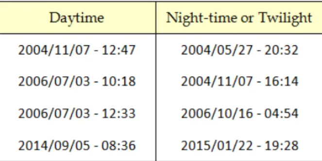
Since the processing paths of both cloud classification softwares and the resulting output interpretation, are affected by the lighting conditions, the different cases are classified also according to this feature (table 4.2), by using the provided SAFNWC flag. So, taking advantage of this information, the scenes can be divided into four cases predominantly or totallydaytime and four cases mainly classified as twilight ornight-time.
Hereafter a brief description of each weather event and of its characterizing physical phenomenon, is presented and completed with the results of the BTD test illustrated in chapter 3. This is a very useful tool to evaluate the cloud vertical development and the possible presence of an overshooting top.
CASE STUDIES
Table 4.1: Case studies selected. These are categorized in three classes by the phenomenon characterizing them, and, for each one the date, AMSU-B/MHS and SEVIRI acquisition UTC times, location and region of occurrence are given. Note that, for the events of 2006/07/03 and 2004/11/07, two times have been taken, showing different stages in the involved system evolution.
Table 4.2: Case studies classified via the SEVIRI illumination flag which character-izes the majority of the involved scenes.
4.1 l o c a l i z e d s y s t e m s c au s i n g f l o o d s
Vibo Valentia - 2006/07/03
On July 3rd 2006 exceptional and intense rainfall affected central Calabria lasting a few hours. A rain gauge in the city of Vibo Valentia registered more than 200 mm of rain in about 2 hours. Such rainfall amount was far above the usual seasonal