A method for robust design of diagrid structures

(1)

POLITECNICO DI MILANO

Department of civil and environmental engineering

Master’s degree in Civil Engineering Track Structures

A method for robust design of diagrid structures

Supervisor: Prof. Capsoni Antonio

Candidate: Lavorini Luca ID n°: 873655

(2)

(3)

Abstract

This work aims to define a method to design robust diagrid for every load condition present in the structure environment and it focuses the attention to diagrids in high-rise buildings, in order to withstand especially lateral loads. Starting with an introduction of the various types of structure and the definition of the robustness requirement, optimization methods are introduced because of their importance in the robust design of structures. When describing the main methods, such as Michell’s truss, principal stresses trajectories and topology optimization, and detailing the last one, it has been observed that they are all connected and lead to the same result, which is a kind of natural layout described by the force flow through the structure volume. Then, understanding the tall building problem, a single load case evaluation of the optimal layout is implemented on a simple example like a square box section cantilever beam under uniform transversal load orthogonal to one face and later, for the robust design, the same system is subjected to a multi-loading case with the same load that rotates around the structure. This last case is the key for robust design, because the wind impact angle is not a defined parameter, but it is the source of uncertainty that characterizes the robustness. It is then demonstrated that the robust layout follow the principal stresses trajectories of the system, a numerical example using those trajectories layout is being proposed to prove the efficiency of the approach and, at the end, some existing practical example are being listed to prove this approach.

(4)

Figures summary

Figure 1.1 Vladimir Shukhov [1853-1939] (right), Shukhov tower in Polibino [1896] (left) ... 1 Figure 1.2 30 St Mary Axe, called "the Gherkin", London, United Kingdom, by Foster and Partners ... 3 Figure 1.3 Guangzhou TV Astronomical and Sightseeing Tower, usually called "Canton tower", Canton, China, by Information Based Architecture (IBA): Mark Hemel and Barbara Kuit ... 4 Figure 1.4 Aldar Headquarters building (right), by MZ Architects, and Capital gate (left), by RMJM, Abu Dhabi, United Arab Emirates ... 5 Figure 2.1 Ronan Point, evidence of the partial collapse (1968) ... 6 Figure 3.1 James Clerk Maxwell [1831-1879] (right), reciprocal diagrams (left) of the structure, (a), and forces (b) ... 10 Figure 3.2 Anthony George Maldon Michell [1870-1959] (right), cantilever problem in a free boundary space (left) ... 12 Figure 3.3 a) principal moments pattern for a slab modulus and b) the Gatti Wool Factory floor ... 15 Figure 4.1 Simply supported beam problem ... 17 Figure 4.2 Sizing optimization solution for simply supported beam problem .. 17 Figure 4.3 Shape optimization solution for simply supported beam problem .. 18 Figure 4.4 Topology optimization solution for simply supported beam problem ... 18 Figure 4.5 General body system ... 19

(8)

Figure 4.6 Mesh dependency of the optimization problem for a simply supported beam, from a) to c) the number of finite elements increases having the same amount of volume ... 25 Figure 4.7 Comparison between layouts with different amount of volume, case a) 30%, case b) 60% and case c) 90% ... 26 Figure 4.8 Cantilever problem, with topology results of volume fraction 20% a), 40% b), 60% c) and 80% d) ... 27 Figure 5.1 3D square section cantilever problem under uniform distributed transversal load with varying direction ... 29 Figure 5.2 Section stress state for 3D square section cantilever problem under orthogonal uniform distributed transversal load, normal stress σz (right) and

shear stress τxz and τyz (left) ... 30

Figure 5.3 2D cantilever problem under in-plane uniform distributed transversal load (right) and section stress state (left) with normal stresses σz

(top) and shear stresses τxz (bottom) ... 32

Figure 5.4 Principal stresses trajectories for 2D cantilever problem under transversal uniform distributed load, tension trajectories (right) and compression trajectories (left) ... 34 Figure 5.5 Cross-section faces names (right) and impact angles (left) ... 35 Figure 5.6 Principal stress trajectories for 3D cantilever problem at impact angle 0° ... 36 Figure 5.7 Principal stress trajectories for 3D cantilever problem at impact angle 22.5° ... 37 Figure 5.8 Principal stress trajectories for 3D cantilever problem at impact angle 45° ... 37

(9)

Figure 5.9 Principal stress trajectories for 3D cantilever problem at impact angle 67.5° ... 38 Figure 5.10 Principal stress trajectories for 3D cantilever problem at impact angle 90° ... 38 Figure 5.11 Bold lines represent shear-lag distribution and the dotted line the Eulerian stresses distribution. The case a) is for sections close to the clamped edge, so in typical shear-lag, while the case b) is close to the free edge, so in negative shear-lag ... 40 Figure 5.12 Section stress state for 3D square section cantilever problem under orthogonal uniform distributed transversal load, normal stress σz with shear-lag

effect (right) and shear stress τxz and τyz (left) which remain invariant ... 40

Figure 5.13 Principal stresses trajectories for 3D cantilever problem at impact angle 0° and shear-lag effect ... 41 Figure 5.14 Principal stresses trajectories for impact angle 0°. Case a) webs for no shear-lag (left) and shear-lag (right), case b) flanges for no shear-lag (left) and shear-lag (right) ... 42 Figure 6.1 Comparison between principal stresses trajectories layout, a), and topology optimization result, b). Adjusting principal trajectories, c), a similar layout is obtained, d). ... 44 Figure 6.2 Comparison between topology optimization, a), and Michell's truss b) ... 45 Figure 6.3 Comparison between topology optimization, a), and Michell's truss b) from Bendsøe and Sigmund book ... 46 Figure 6.4 Comparison between Principal stresses, a), and Michell's truss b) from obtained connecting intersection nodes between trajectories ... 47 Figure 7.1 ABAQUS model, load assignment method ... 50

(10)

Figure 7.2 ABAQUS model, load redistribution ... 51

Figure 7.3 Load dependency of symmetry ... 51

Figure 7.4 ABAQUS model, general direction load repartition ... 52

Figure 7.5 ABAQUS model, final configuration with beam elements ... 53

Figure 7.6 ABAQUS model, single load natural symmetry ... 54

Figure 7.7 ABAQUS model, SIMP results for single load case, general overview ... 54

Figure 7.8 ABAQUS model, SIMP results for single load case, web side view . 55 Figure 7.9 ABAQUS model, SIMP results for single load case, flange side view ... 55

Figure 7.10 ABAQUS model, with single load equal faces and imposed symmetry ... 56

Figure 7.11 ABAQUS model, SIMP results with single load equal faces and imposed symmetry, general overview ... 57

Figure 7.12 ABAQUS model, SIMP results with single load equal faces and imposed symmetry, side overview ... 57

Figure 7.13 ABAQUS model, general view of multi-load topology result ... 58

Figure 7.14 ABAQUS model, façade layout from multi-load topology result ... 59

Figure 8.1 Diagrid configuration for web layout, lines with starting point pitch, from left to right at H/B, H/2B, H/4B, H/8B, H/16B. Configuration without shear-lag (top) and with shear-shear-lag (bottom) ... 62

Figure 8.2 Grasshopper modelling comparison for three layouts in 2D, web layout (right), flange layout (centre), regular layout (left) ... 64

(11)

Figure 8.4 Grasshopper modelling, deformed configurations ... 66

Figure 8.5 Grasshopper modelling, 3D models, web model (left), PST model (middle) and regular model (right) ... 67

Figure 8.6 Grasshopper modelling, load cases, 0° (left), 45° (middle) and 90° (right) ... 68

Figure 8.7 Transbay tower competition, San Francisco, California, designed by SOM ... 71

Figure 8.8 a) Principal stress trajectories layout concept, from Beghini et all [OPTIMIZATION] and b) the Kunming Junfa Dongfeng Square, Yunnan, China, designed by SOM ... 71

Figure 8.9 CITIC Financial Center, designed by SOM ... 72

Figure 8.10 Burj-Jumeira tower, Dubai, designed by SOM ... 72

Figure 10.1 Cantilever system for shear-lag computation ... 97

Figure 10.2 From Stromberg at all paper, a) is the case of a meshed rectangle under a set of transversal load, and b) is the same system but with the contribution of vertical beams at each lateral side ... 124

Figure 10.3 ABAQUS model, results from the first topology analysis without beam elements ... 125

Figure 10.4 Diagrid evaluation for columns pre-sizing ... 126

Figure 10.5 ABAQUS model, Continuum-Beam model ... 127

Figure 10.6 ABAQUS model, cylinder model ... 128

Figure 10.7 ABAQUS model, four clamped points general view ... 129

Figure 10.8 ABAQUS model, four clamped points lateral view ... 130

(12)

Figure 10.10 ABAQUS model, eight clamped points lateral view ... 131 Figure 10.11 ABAQUS model, sixteen clamped points general view ... 131 Figure 10.12 ABAQUS model, sixteen clamped points lateral view ... 132

(13)

1

1. An introduction to diagrid structural

systems

The word diagrid is a portmanteau of “diagonal grid” and in the field of structural engineering gives the noun to a structural framework of diagonal intersecting beams, which may be made by one or more materials. This bearing system is often used in buildings and roofs for its efficiency in term of stiffens and material costs, because it usually requires less material that another system configuration.

Nowadays, a widespread application of diagrids is in large span and high-rise buildings, where due to the large-scale system the reduced costs have been hugely highlighted.

(14)

2 The origin of “diagonal structures”, as described by architect Ian Ritchie [47], is the work made by the Russian genius Vladimir Shukhov [1853 – 1939], who pioneered new analytical methods in many different fields. Shukhov left a considerable legacy to early Soviet Russia constructivism leading engineers to the design of hyperboloids, thin shells and tensile structures of extraordinary refinement and elegance basing on diagonal members mechanisms. One of his most famous diagrid systems, which should be considered the “father” of diagrid structures, is the Shukhov tower in Polibino, designed in 1896 and built between 1920 and 1922. It represents the essence of this kind of structure, having no vertical elements, being slender and lightweight.

Focussing on tall buildings, the study of diagrids gets a spark to develop new concepts and applications. The most influencing actions in high rise building design are the lateral loads mostly given by wind and earthquake, which are carried by exterior or interior structural systems. The diagrid is one of the most common solution for this purpose due to its duality in structural efficiency and architectural advantages, both aesthetically and functionally speaking.

(15)

3 Figure 1.2 30 St Mary Axe, called "the Gherkin", London, United Kingdom, by Foster and Partners

Commonly, the diagrid is made by diagonals elements only and doesn’t require any vertical column, because the inclined members, intersecting each other, bear both shear and overturning moment effects, acting as “inclined columns” and bracing elements”. Over the years, it has been presented a solution for both vertical and lateral actions, which confirm a reduction of material costs, estimated around 20% compared to conventional moment-frame structures[7].

Apart from evident costs advantages, the diagrid system allows a large use of glass façade which, form a comfort point of view, allows a generous amounts of day light into the building. Furthermore, it represents one of the most feasible solution in terms of energy efficiency and low environmental costs, which represent nowadays some of the main topics for a sustainable design.

(16)

4 Figure 1.3 Guangzhou TV Astronomical and Sightseeing Tower, usually called "Canton tower", Canton, China, by Information Based Architecture (IBA): Mark Hemel and Barbara Kuit As every structural solution, diagrids present some drawbacks or demerits. The noted complications are focussed on glasses modelling, nodes fabrication and construction. The first point is quite evident, because it involves irregular shapes and windows sequences, while the other two, that are more technical, request adequate sources.

By the way, as every structure, diagrids are not exempt from technical considerations. Their features of being versatile and aesthetically pleasant are “intrinsically” fixed into the proposed configuration, but the structural efficiency still depends on the designer ability to imagine the real environment impact during the structure life.

(17)

5 Figure 1.4 Aldar Headquarters building (right), by MZ Architects, and Capital gate (left), by RMJM, Abu Dhabi, United Arab Emirates

This work will focus on diagrid system on high-rise buildings and where the most significant environmental effect is given by lateral loads, which will be considered purely as wind actions. Being the wind and earthquake directions unpredictable, the efficiency of the diagrids is not evaluated on classical design actions only, but it takes into account the uncertainty related to loads, generating a elements layout that may have the best performance for every circumstance. This capacity is called “structural robustness”, and being related to the best performance, it is also strictly related to “optimization design approaches” which are used to determine the most efficient layout of systems.

(18)

Knowing the type of structure that is involved, the next step for a designer is to catch the philosophy that withstand behind his design choices. So, what is exactly the structural feature called “robustness” and how it exists into the structure environment.

(19)

5

2. About the idea of structural robustness

The adjective “robust” takes its origins from the Latin world, where the term “robustus”, from “robur” and earlier “robus”, has the meaning of strength, sturdy or hardy, and gives also the name to oaks trees, for their resistance and their red colour on leaves, “rubeus”, which is symbol of blood and life. As this last reference suggests, this adjective is used for subjects able to resist to different or adverse conditions far from the average one, or, in other words, to withstand against ad huge number of situations, like life presents.

Over the years the noun “robustness” is then used referring to the same root of strength and it is introduced in various knowledge fields indicating, as Woliński suggested [58], the property of a system to survive unforeseen or extraordinary exposures or circumstances that would cause failure or loss of functionality.

Almost every science defines in their fields this particular attitude in special subjects, for example in biology the idea of robustness has been used in field of evolution, meaning the persistence of a system’s characteristics after perturbation, and in morphology we define as robust species with a body-system based on strength. Moving to more practical studies, like economy, the word finds its meaning as the ability of a financial trading system to remain effective under different markets conditions, or in computer science, as the ability of a computer system to deal efficiently with errors, from the execution or from input, that should occur in every moment.

On the other hand, in more mechanical engineering field, such as civil, mechanical or aerospace, the term robustness has different meanings gravitating around the same root, and the definitions itself sometimes is one of the main issues, as Banu said [6]. Following literature and codes, two flow-ideas emerge to establish the body of such property.

(20)

6

2.1.

Robustness as structural collapse resistance

In the most classical sense robustness is a structural requirement not to let the partial collapse of structure component doesn’t cause or induce the global or partial collapse of the structure or using the words by Starossek and Haberlad [51], it is “a desirable property of structural systems which mitigate their susceptibility to progressive or disproportionate collapse”. The need to “control” in some way the partial collapse of a structure in order to prevent a much more global functionality and safety born during the last years of the XXth century, when on 16 May 1968 the tower block Ronan Point lost one entire corner along the height due to a local explosion.

Figure 2.1 Ronan Point, evidence of the partial collapse (1968)

The cause was a gas explosion in the kitchen of an 18th floor flat which resulted in the collapse of the entire south-east corner of the 22-storey east London tower block, killing four people and injuring seventeen. The disaster led to a loss of public confidence in high-rise residential buildings and resulted in major changes in UK building regulations on 1970. According to Pearson and Delatte

(21)

7 [9], from that point British government manded guidelines for the prevention of progressive collapses, these instructions including the requirement of fail-safe mechanism and require that under specified loading conditions a structure must remain stable with a reduced safety factor in the event of a defined structural member or portion thereof being removed. The lessons from Ronan Point changed building regulations throughout the world and over 50 years after the collapse every code around the nations presents sections which stress the idea of structural integrity and the aim to design so that structures sustain local damage with the system globally remaining stable. This requirement, at the end, takes the name of structural robustness, but even after all that safety goals it doesn’t exist and unique definitions or description, neither a formula to compute it. It is strictly related to the probability of progressive collapse and the risk to special event occurrence, which allows to determinate the probability of collapse resistance, but there is no proper robustness parameter evaluation for that requirement. Mentioning the Eurocode definition, in “BS EN 1991-1-7 Actions on structures. General actions, Accidental actions” [8], it is written:

“Robustness is the ability of a structure to withstand events like fire, explosions, impact or the consequences of human error without being damaged to an extend disproportionate to the original cause.”

2.2.

Robustness as best performance for every situation

Another way to define the structural robustness is related to the idea that the undamaged structure use to resist in the most optimal way to all possible load situations which were not included in the design process, like, for example in tall buildings, all possible wind blowing directions or earthquake action directions. This point of view born realizing that the world is full of uncertainties and structures need, following Dunning at al. [42], to be designed and optimized to be robust when operating in an uncertain environment. The traditional engineering approach to account for uncertainties is to employ a factor of safety. While this philosophy has produced many successful structures, the modern era

(22)

8 demands more efficient designs that minimize waste in order to meet pressures from both economic and environmental factors. In this context the safety factor approach may be inadequate and, taking into account, for example, the considered design loads, the load directions and their magnitude should be the source of uncertainty. Then, as Csébfalvi says [11], the investigation of the most optimal structure design, and so the most robust one, is frequently sensitive to the directional uncertainties of the applied loads. The hardest question is then, which is the optimal layout of material that guarantee the best performance to an uncertainty environment?

Summarizing those two orientations of robustness in structures, we have from one side a sufficient performance in terms of functionality in damaged situations, which is necessary for safety reasons as history has shown, and from the other the ability to behave in the most optimal way to the whole possible load situations. This last requirement is the one that matches the initial definitions of robustness and is the one that defines the guide lines for the best design, and that influences also the other robustness requirement.

(23)

The description could move on describing in detail the relations that withstand between robust design and optimal design, and the methods to investigate this last performance requirement.

(24)

9

3. Optimization problem history

The optimization problem in structural engineering usually concerns material disposition of a volume. This study is about the philosophy which manages the material distribution in a given space, standing into given system constrains and following the aim of best performances.

The investigation of the optimal design layout is a requested target nowadays in building industries, especially in high-rise buildings, due to, as Sarkisian at al. declare [35] the least amount of material goal for economic and environmental reasons. It must be noted that behind those motivations the least material amount techniques are often used because of the duality between pleasant aesthetic from an architectural point of view, and optimal efficiency.

3.1.

Maxwell’s theorem and Michell’s trusses

The theory about structural optimization born more than una century ago, when the problem itself was focussed on truss structures configurations, and it evolved till modern era in more general approaches on continua under various targets. The earlier works about optimization are attributed to Rankine (1858), who generalized the equilibrium solution of funicular systems, and Maxwell (1870), about the minimum volume of a truss layout under given loads. Both theories are based on graphical approaches and even if they started the investigation of optimality through the time it has been lost their application, till the end of the XX century. Some of the most recent applications of the works of Rankine include method for cable systems, as they are presented in Beghini et al papers [1].

At the beginning the aim of optimal structural design was to find truss structure configurations in order to get the stiffest configurations under the least amount of material. The first work which paves the way to that path was proposed by James Clerk Maxwell [1831-1879] with “On reciprocal figures, frames, and

(25)

10

diagrams of forces”, published in 1870 [36], where it is provide quick method to

establish the minimum volume of a frame under a given set of loads and boundary conditions.

Figure 3.1 James Clerk Maxwell [1831-1879] (right), reciprocal diagrams (left) of the structure, (a), and forces (b)

As Lógó et al clearly describe [22], Maxwell in his paper proposed a theorem about the equilibrium of a series of attracting repelling centres of force and applied it to trusses, where the bars replaced the action at a distance except in the case of the external forces. Mentioning Maxwell’s words upon scientific significance of his theorem:

‘‘The importance of the theorem to the engineer arises from the circumstance that the strength of a piece is in general proportional to its section, so that if the strength of each piece is proportional to the stress which it has to bear, its weight will be proportional to the product of stress multiplied by the length of the piece.

(26)

11

Hence these sums of products give an estimate of the total quantity of material which must be used in sustaining tension and pressure respectively.”

It must be noted that Maxwell uses the word ‘‘stress” for what we should term ‘‘load”.

The problem itself should be described as follows.

Taking a truss structure in equilibrium under a set of forces Fi acting at the points ri, (i = 1, 2…, n) and dividing tension members and compression members with length, section areas and applied load respectively Lt, At, Tt, and Lc, Ac, Tc. Defining admissible stresses as ft and fc, respectively, by the principle of virtual work the optimality condition of the lightest structure is derived, and it has the volume given by:

𝑉 = 𝑉_𝑐(1 +𝑓𝑐 𝑓_𝑡) + 1 𝑓_𝑡∑ 𝐹𝑖𝑟𝑖 𝑖 = 𝑉_𝑡(1 +𝑓𝑡 𝑓_𝑐) − 1 𝑓_𝑐∑ 𝐹𝑖𝑟𝑖 𝑖

Here Vt and Vc are the volume of all the tension and compression members respectively.

Later in 1904, Anthony George Maldon Michell [1870-1959] generalized the Maxwell’s theorem and applied it in order to establish the formulation for the optimum structural weight of a truss. Even if Maxwell has exposed clearly the need of optimal layouts, the Michell work, “The limits of economy of material in

frame-structures” [38], is today considered the starting point of structural

optimization theories.

He listed a set of conditions for a structure to be an optimum and proved the geometric restriction which determines the classes of orthogonal sets of curves along which the members of an optimum structure must lie.

(27)

12 Starting from the Maxwell’s problem, referring to a set of external forces Fi acting at the points ri, (i = 1, 2…n). Let D be a space domain which includes the points ri and the whole of feasible space. Now, considering the all possible frameworks, trusses systems, S, contained in D, which equilibrate the forces Fi and which satisfy the stresses limiting, it is assumed that there is a framework

S* which satisfies the following condition of Michell:

‘‘There exists a virtual deformation of the domain D such that the strain along all members of S* is equal to ±e, where e is a small positive number, and where the sign agrees with the sign of the end load carried by the particular member, and further that no linear element of D has strain numerically greater than e.”

Figure 3.2 Anthony George Maldon Michell [1870-1959] (right), cantilever problem in a free boundary space (left)

The statement of the theorem is that the volume V* of S* is less than or equal to the volume V of any of the other possible frameworks S.

𝑉 =𝑓𝑡+ 𝑓𝑐 2𝑓_𝑡𝑓_𝑐 (∑ 𝐿𝑡𝑇𝑡 𝑡 + ∑ 𝐿𝑐𝑇𝑐 𝑐 ) −𝑓𝑡− 𝑓𝑐 2𝑓_𝑡𝑓_𝑐 ∑ 𝐹𝑖𝑟𝑖 𝑖

(28)

13 Then, the volume V* is derived from the principle of virtual work, where, if the virtual displacements, corresponding to Michell’s statement, are evi at ri, this volume V* is: 𝑉∗ =𝑓𝑡+ 𝑓𝑐 2𝑓_𝑡𝑓_𝑐 ∑ 𝐹𝑖𝑣𝑖 𝑖 −𝑓𝑡− 𝑓𝑐 2𝑓_𝑡𝑓_𝑐 ∑ 𝐹𝑖𝑟𝑖 𝑖

The imposed deformation e imposes certain restrictions on the final layout in

S*. Citing Lógó et al paper:

“At a node of this framework the directions of the strains ±e, which are along the lines of members of S* and are principal directions of strain and must satisfy certain orthogonality conditions. In a three-dimensional truss, at a node with three members, there are no restrictions, if the load in members have the same sign, since in that case the virtual deformation is a pure dilatation and therefore isotropic. If one load is of opposite sign to the others, it must be at right angles to them. For a node with four members, there is again no restriction if all the loads have the same sign. If one member has an opposite load to the other three, then it must be orthogonal to them all and so forces them to lie in a plane. Finally, if the members fall into pairs with opposite-signed loads then one of these pairs must be in line and normal to the other two.”

Moving from the advantages of using the least amount of material, the most important property taking from Michell work is that when we obtain the optimal configuration, the optimal structure itself, S*, has also the greater grade of stiffness that any other structures in the S range.

Anyway, it is noted that the original Michell formulas are not valid for different allowable stresses in tension and compression. Only in 1960 Chan [10] wrote down correctly the Michell’s theorem and the validity and the critical examination of the Michell’s theory can be read in Rozvany’s work [48] also, almost 40 years later.

(29)

14

3.2.

Evolution of optimization methods

From those analytical theories applications on engineering have raised together with related problems and discussion. Firstly, in 1958, it was presented the non-uniqueness of the optimal layout, by H. L. Cox, in terms of minimum weight, since he demonstrated the existence of different configurations with the same weight. So, the optimal solutions are not unique in the case of Michell’s structures. Using variational calculus Shield, later in 1973 presented some additional conditions for the stationarity of the structural volume but even with these addictions it was not possible to guarantee a global optimum layout. Shield working on the Michell’s structures declared that this design fails when kinematic constraints are taken into consideration, and so he chooses to propose an alternative approach which has not that limits.

The investigation about the convergence of solution and its uniqueness are of primary importance and their achievement remains more complicated if are presented multiple load cases or loading uncertainty is considered. The load can be considered as a quantity given in an interval with a certain possibility of location or/and direction, and/or magnitude, and they are selected depending on the worst effects. This topic was investigated in analytical ways by Nagtegaal and Prager in 1973.

3.3.

Principal stresses trajectories

Since the Cauchy tensor has been formulated, the existence of specific orientations, for every single infinitesimal element where no shear stresses exist and only axial stresses leads, was known. Those directions, principal directions, map a series of trajectories that define the force flow into the body from its entrance to the constraints. Studying those lines, it was noted that some natural elements follow them, for example bones pore structure in human body, and this naturally offers a guideline to use the whole material properties. There are no specific examples or a starting point of this theories, but one of the most

(30)

15 famous application of this approach, to obtain optimality in terms of stiffness and material economy, was the Gatti Wool Factory, in 1953, by Pier Luigi Nervi [1891-1979]. After similar works, he proposed a ribbed floor system where ribs follow principal moment directions of the slabs, around the support system made by columns. Those were isostatics lines where no torsional moment exists and intersect each other orthogonally for the hole pattern. This approach is described in detail by Halpern at all [4] where the so called “Nervi’s method” is presented in new forms.

Figure 3.3 a) principal moments pattern for a slab modulus and b) the Gatti Wool Factory floor On the other hand, as it will be seen during this work, those approach with principal stresses trajectories is often used nowadays for its efficiency but also because its aesthetics.

3.4.

Material distribution methods

Till now it has been defined a macroscopic theory about optimization base on trusses elements, boundary conditions and loads and it allows mainly to define sizes and sections of the members itself. By the way, a microscopic approach naturally arose for shape and sizing optimizations, for and higher freedom on the form management and because the microscopic approach allows engineers

(31)

16 to study the relations between the microstructure itself and the macrostructure behaviour. This was for example clearly demonstrated in the paper by Cheng and Olhoff in 1981, on optimal thickness distribution for elastic plates, which started clearly in some way a marked interest in microscopic material distribution.

From the introduction of Finite Element Methods (FEM) in engineering word, optimization theories have changed their solution approach ad many analytical problems, in terms of computations, have been overpassed, as Lucien Schmit, in 1960, recognized. The trend of numerical evaluation, instead of analytical one, has affirmed its position in research and design world. From that point the microstructure approach, or material distribution method, found its proper tool for numerical evaluations and experiments and enter completely in the practical word in 1988 from the first paper by Martin Philip Bendsøe et al [34], who defines a computational tool.

To complete the introduction and the continuing of the optimization analytic it is appreciable mentioning Bendsøe and Sigmund [34], from their book “Topology

optimization: theory, methods and applications”:

“For thin structures, that is, structures with a low fraction of available material compared to the spatial dimension of the structure, the material distribution method predicts grid- and truss-like structures. Thus, the material distribution method supplements classical analytical methods for the study of fundamental properties of grid like continua, as first treated by Michell. Applications of numerical methods to truss problems and other discrete models were first described in the early sixties but now we see that these challenging large-scale problems can be solved with specialized algorithms that use the most recent developments in mathematical programming. In its most general setting shape optimization of continuum structures should consist of a determination for every point in space if there is material in that point or not. Alternatively, for a FEM discretization every element is a potential void or structural member. In this

(32)

17

setting the topology of the structure is not fixed a priori, arid the general formulation should allow for the prediction of the layout of a structure. Similarly, the lay-out of a truss structure can be found by allowing all connections between a fixed set of nodal points as potential structural or vanishing members.”

(33)

From the born of a such versatile approach as material distribution methods the optimization studies discovered new frontiers and more versatile solutions. Is then necessary focussing a little bit the attention on that method

(34)

17

4. Material distribution method – Topology

optimization by minimum compliance design

The three main optimization problems, which address different aspects of the structural design problem, are the sizing, shape and topology methods.

Figure 4.1 Simply supported beam problem

The sizing problem leads to find for example the optimal thickness distribution on a linear elastic plate or the optimal elements area in a truss structure, design variables, in order to minimize or maximize one or more physical targets, state variables, such as strain energy, maximum stress, deflection etc. The main characteristic of this approach is that the design model domain and the state variables are defined a priori and are fixed during the process.

Figure 4.2 Sizing optimization solution for simply supported beam problem

In the shape problem, instead of sizing, as the noun suggests the scope is the research of the optimal shape of the domain and that design space becomes a design variable.

(35)

18 Figure 4.3 Shape optimization solution for simply supported beam problem

At the end, the topology optimization problem, which is the more versatile and general, is focussed on defining the number, shape and location of “holes” into de design domain and also its connectivity.

Figure 4.4 Topology optimization solution for simply supported beam problem

With this last method is possible to define the optimal layout of a structure having few information, such domain, loads and constraints, and so it represents the most versatile approach to study the nature of a mechanical system.

4.1.

Method description

The topology optimization problem is to determine, under a defined space region, the optimal layout, in terms of performances, standing on some known conditions, such as applied loads, supports, structure volumes and others sub requirements. So, the size, the shape and the connectivity of the final product are usually unknown or should be supposed in few cases from theories. For the purpose of this work only the simplest case of isotropic material and minimum compliance criterion is considered. With the term compliance we refer to the strain energy of a mechanical system, an indirectly to its displacements, so it is the inverse of the system stiffness. Indeed, minimizing the compliance of the problem is the same to maximise the stiffness of the problem and this concept will be stressed more later.

(36)

19 Figure 4.5 General body system

Considering a source domain Ω, in R3_{or R}2_{, of an isotropic material, in which it} is contained a “target” domain Ωmat, on which volume and surface loads, f, are applied, and constrains are imposed, Γu. There should be also some void region or fixed solid region, Ωe and Ωf. The optimal design problem is defined as the investigation of the optimal stiffness tensor Eijkj(x), which can vary into the source domain. Writing the bilinear form of energy, where u is the equilibrium configuration and v the virtual displacement:

𝑎(𝑢, 𝑣) = ∫ 𝐸𝑖𝑗𝑘𝑙(𝑥)𝜀𝑖𝑗(𝑢)𝜀𝑘𝑙(𝑣)𝑑𝛺 𝛺 and 𝜀𝑖𝑗(𝑢) = 1 2( ∂𝑢_𝑖 ∂𝑥𝑗 +∂𝑢𝑗 ∂𝑥𝑖 )

About the load work in linear form:

𝑙(𝑢) = ∫ 𝑓𝑢𝑑𝛺

𝛺

+ ∫ 𝑓𝑢𝑑Γ_𝑇

(37)

20 The problem is then formulated as the investigation of the minimum strain energy or minimum compliance problem, and then it implies that the system configuration with the minimum deformation is also the stiffest in the whole possible configurations. So, working intrinsically on a maximum stiffness problem, the formulation is then written as:

𝑚𝑖𝑛

𝑢∊𝑈,𝐸 𝑙(𝑢)

𝑠. 𝑡. 𝑎𝐸(𝑢, 𝑣) = 𝑙(𝑣)

𝐸 ∊ 𝐸𝑎𝑑

for all 𝑣 ∊ 𝑈

Where U is the space of the kinematically admissible displacements and Ead is the set of all admissible stiffness tensor for the design problem in the unknow

Ωmat configuration. It must be underlining that the stiffness tensor E has zero value outside the admissible set and that the limit resource of the problem is expressed by the target volume, defines as:

∫ 1𝑑𝛺

𝛺𝑚𝑎𝑡

≤ 𝑉 = ∫ 1𝑑𝛺

𝛺

When the problem is solved by computational approach, discretizing the continuum by FE for example, the parameters previously defined are also discretized, and introducing the corresponding quantities the formulation becomes: 𝑚𝑖𝑛 𝑢∊𝑈,𝐸 𝑓 𝑇_𝑢 𝐾 = ∑ 𝐾_𝑒(𝐸𝑒) 𝑁 𝑒=1 𝑠. 𝑡. 𝐾(𝐸𝑒)𝑢 = 𝑓 𝐸𝑒 ∊ 𝐸𝑎𝑑 for

(38)

21 Where K is the stiffness matrix of the whole system generated by the stiffness contribution of every single element e =1, …, N, which depends on the single element stiffness Ee.

Having now a discretized space in FE the next step is to determine which points of that space are material points and which are void points. For the formulated problem described above, this implies that the set of admissible stiffness tensors,

Ead, has the property:

𝐸𝑖𝑗𝑘𝑙 = 1𝛺𝑚𝑎𝑡𝐸𝑖𝑗𝑘𝑙0 where 1𝛺𝑚𝑎𝑡 = {1 0 𝑖𝑓 𝑥 ∈ 𝛺𝑚𝑎𝑡 𝑖𝑓 𝑥 ∈ 𝛺 𝛺⁄ 𝑚𝑎𝑡 ∫ 1_𝛺𝑚𝑎𝑡𝑑𝛺 𝛺 = 𝑉𝑚𝑎𝑡 ≤ 𝑉 = ∫ 1𝑑𝛺 𝛺

The last relation expresses a limit on the amount of material, defined as a fraction of the initial source volume, in which the compliance must be minimized. The tensor E0ijkl defines the stiffness tensor of the isotropic material and the admissible tensor under this condition results as a distributed and discrete valued design problem, or 0-1 problem. Anyway, to solve that problem, commonly, integer variables 0-1 are not suggested and then they are replaced with continuous values between the previous edges by the introduction of a factor which steers the process as much as possible to the 0-1 type.

The design problem is then solved modifying the stiffness matrix so that it depends continuously on a function interpreted as the density of the material, stressing the idea that the optimization is a problem of regions with and without material. For the values of the tensor that are between 0 and 1, due to that new factor of continuity, are considered as “artificial” density values and then, in order to mitigate correctly their contribution, they are penalized in some way.

(39)

22

4.2.

SIMP method

There are many methods that follows that approach, but the most popular and stable is the “Solid Isotropic Material with Penalization”, SIMP, or penalized proportional stiffness model, which is formulated as:

𝐸_{𝑖𝑗𝑘𝑙}(𝑥) = 𝜌(𝑥)𝑝_𝐸 𝑖𝑗𝑘𝑙0 where 𝑝 > 1; 0 ≤ 𝜌(𝑥) ≤ 1 𝑥 ∈ 𝛺 ∫ 𝜌(𝑥)𝑑𝛺 𝛺 = 𝑉𝑚𝑎𝑡 ≤ 𝑉 = ∫ 1𝑑𝛺 𝛺

The “artificial density” ρ(x) is the design function, with values between 0 and 1, and E0ijkl represent the properties of the isotropic material as always. At the extreme of its interval, ρ(x) gives to the stiffness tensor the values:

𝐸𝑖𝑗𝑘𝑙(𝜌 = 0) = 0 𝐸𝑖𝑗𝑘𝑙(𝜌 = 1) = 𝐸𝑖𝑗𝑘𝑙0

So, imaging the source space as a grid of squares, the final result is a map of white (no material), black (full material) and grey (partial material) squares, where this last typology, if the problem converges perfectly, disappear from the system.

The penalty factor p is choosing greater than 1 and mathematically speaking, for intermediate values of density, it gives for those elements an unfavourable value of stiffness compared to the full material elements. So, the choice of the penalty factor determines directly the convergence and quality of the final layout solution.

Being this a computational model, the need to find a physical meaning of its result naturally arise especially when the solution doesn’t converge clearly and there are some “grey” regions that must be interpreted. To guarantee a physical

(40)

23 material model meaning to SIMP, there have be found limits values for penalty factors, for 2D and 3D problems:

𝑝 ≥ 𝑚𝑎𝑥 { 2 1 − 𝜐0; 4 1 + 𝜐0} 2D models 𝑝 ≥ 𝑚𝑎𝑥 {15 1 − 𝜐 0 7 − 5𝜐0; 3 2 1 − 𝜐0 1 − 2𝜐0} 3D models

Where υ0_{is the Poisson’s ration. In the most general cases the limit value to} obtain a reasonable result is for 2D cases “3” and for the 3D cases “2” but is a convention for both cases taking a penalty factor of “3” at least.

Working with FEM analysis, to complete the explanation the FE form of the final problem is given:

𝑚𝑖𝑛 𝑢,𝜌𝑒 𝑓 𝑇_𝑢 𝑠. 𝑡. (∑ 𝜌_𝑒𝑝𝐾_𝑒 𝑁 𝑒=1 ) 𝑢 = 𝑓 ∑ 𝜐_𝑒𝜌_𝑒 𝑁 𝑒=1 ≤ 𝑉, 0 < 𝜌_𝑚𝑖𝑛≤ 𝜌_𝑒 ≤ 1, 𝑒 = 1, … , 𝑁

In order to avoid singularities is commonly introduced a lower bound value for the density, ρmin, at 10-3.

4.3.

Solving procedure

To solve the problem, an iterative procedure is proposed, where for each previously computed design and its associated displacements it update the

(41)

24 design variables at each point or FE, independently from any other updated at other points or FE, based on the necessary conditions of optimality.

For a general overview of the process, the topology design on material distribution method with an isotropic material the computational steps are divided in three groups:

Pre-processing

Chose reference domain, load, boundary conditions, region of the process, volume fraction target, sufficiently fine meshing.

Optimization

Basing on displacement finite element analysis, computing the first analysis on the uniformly distributed isotropic material the minimum compliance is solved a new configuration is obtained. The process continues till a marginal improvement target.

Post processing

Interpretations of material distribution results and representation.

The reason why the displacement analysis of each element is considered is because implicitly through the equilibrium equations and relative derivatives they are computed in respect to the design variables of the problem in terms of sensitivity analysis.

For more information about methods, programming and construction details of the methods it is suggested referring to the literature book by M. P. Bendsøe and O. Sigmund, “Topology optimization – Theory, methods and applications” [34].

(42)

25 In addition, all the following 2D topology optimization pictures have been obtained by a MatLab code given by O. Sigmund, [40], typically used for academic purposes.

4.4.

Mesh dependency

Some important aspects on results quality have been detected during the years focussing on some dependency of the method. Firstly, this approach depends strictly in the problem modelling, in particular to its load applications and meshing. The first influences the results, as it will be show later, mostly for symmetrical requirement output or trace of the load application on the final body. The second point, instead, is an important aspect for results purposes.

The mesh dependence of the solution is strictly related to the capacity action of the process during the analysis in such small or not part of the body and it often influences also the existence of solutions. Refining the mesh, the process can operate in a more microstructure way, ideally reached if the mesh is infinitely small, and the holes created in the domain are not large enough but subdivided in many smaller holes creating a fine curtain of elements. The reason of this choice by the process is that with the same values of volume fraction, a structure with a large number of holes, that define a kind of grid, is stiffer that one with a single hole with the same volume dimensions.

Figure 4.6 Mesh dependency of the optimization problem for a simply supported beam, from a) to c) the number of finite elements increases having the same amount of volume

(43)

26 So, increasing the mesh refinement a more detailed structure is achieved. For some purpose, this property is not desirable, like in many mechanical and aerospace projects, where producing an object with such detailed parts is impossible and inconvenient; in this case this feature is covered by filtering actions on the space of density changing, in order to manage the process in a simplest result and less detailed. On the other hand, for large scale systems, a more detailer solution is desirable, because a simpler solution like case a) in leads too much big elements, non-feasible with realizations.

4.5.

Analogy between different volume fractions cases

It must be observed now how the body changes his configuration depending on volume fraction and, in reason of that, how a simpler truss configuration is just the “less material layout” of a finer and more detailed configuration given by a “more material layout”.

Figure 4.7 Comparison between layouts with different amount of volume, case a) 30%, case b) 60% and case c) 90%

(44)

27 It has been noted that decreasing the volume fraction, a simple truss with a minimum number of cells is obtained, but increasing the volume fraction the number of cells tends to grow. From a fraction of 0.3 to 0.6, considering the example in the figure, the number of cells quite duplicates, and the elements become thicker, but passing to a higher fraction like 0.9, the truss part remains more detailed. In general, also considering the case presented in figure, a more complex layout like case c) in both figures, is the detailed version of a simpler one made by a lower fraction of volume.

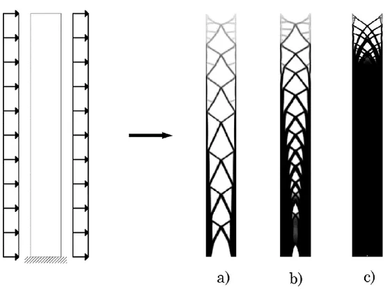
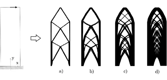
The previous example is affine to the structure quant will be analysed later, but to give a much clear explanation of this analogy between a truss tube and a fine diagrid let consider a stocky cantilever, so that the topology gives clearer diagrids:

Figure 4.8 Cantilever problem, with topology results of volume fraction 20% a), 40% b), 60% c) and 80% d)

The simple layout obtained for a fractal around 20% of the total volume is just a “primitive form” of a finer configuration that emerges for larger amount of material.

(45)

28

4.6.

Multi-load case implementation

A general overview of the topology optimization problem has been given, then some more specific case study should be considered. In order to find the optimal material distribution of a robust structure, more than one load case must be considered, and the design criterion of the topology process must be modified.

The single load case of minimum compliance problem should be easily extended to a multiloading problem, where a minimization of the weighted average of the compliances of each load is computed. The continuum formulation then becomes:

𝑚𝑖𝑛 𝑢∊𝑈,𝐸∑ 𝑤 𝑘_𝑙𝑘_(𝑢𝑘₎ 𝑀 𝑘=1 𝑠. 𝑡. 𝑎_𝐸(𝑢𝑘_{, 𝑣) = 𝑙}𝑘_(𝑣) _{𝑓𝑜𝑟 𝑎𝑙𝑙 𝑣 ∊ 𝑈, 𝑘 = 1, … , 𝑀} 𝐸 ∊ 𝐸𝑎𝑑

Where the index k refers to the k-th load case on the set of M load cases. The factor w is the weight. Again, for more details about the programming phase and mathematical procedures it is suggested referring to the previous mentioned test book by M. P. Bendsøe and O. Sigmund.

During those years, anyway, other methods have been implemented to catch multi-loads results, in particular to reduce the amount of computations. The most popular techniques are proposed by Kai A. James at all [26], with the dynamic aggregation process, and by Zouhour Jaouadi at all [62], by the Epsilon method. This last in particular reduce the amount of computations because bases the process considering the minimization of the load configuration with the maximum compliance value.

(46)

The following parts aim to describe an approach to determine an optimal and robust diagrid layout for high-rise buildings in order to bear the lateral loads mostly given by wind loads. To lighten the procedures an easy and simply tall building is used, but the considerations should evolve for more complicated cases. First, a high-rise buildings analysis description will be proposed.

(47)

29

5. High-rise buildings mechanics

Before starting with the design explanations, it is necessary to understand the overall mechanical behaviour of high-rise buildings.

5.1.

Problem introduction

The problem of high-rise building design is mostly a cantilever beam problem, which is fixed at the base, and due to this fact, the system is statically determinated the main laws governing the problem are simple. So, the state of internal stresses is easily computed once the load set is defined.

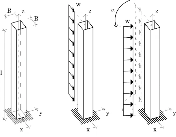
Figure 5.1 3D square section cantilever problem under uniform distributed transversal load with varying direction

The structure under analysis is a tube, height H, with square section of side B and a slenderness ratio, B:H, of 1:8.

(48)

30 By the goal of this work, the problem becomes much simpler because is focussed on lateral load systems of the building and the transverse load analysis determine the overall response. The main lateral load considered is the wind action, which is also the variable parameter that determines the robustness problem due to its direction uncertainty. Knowing from classical literature that the wind load distribution depends in general on the wind velocity, roughness of the space around the building and transverse and tangential effect, the load is simplified as a shard of uniform distributed load enough to catch in a good way the overall behaviour.

As explained in the first part, the principal stresses trajectories are a good guide line to understand the behaviour of a structure and implicitly they suggest the material positions for maximum stiffness and minimum weight. Then, to conclude, principal stresses trajectories are taken under analysis.

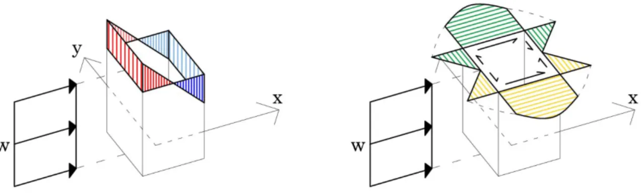
As remarked, from classical structural mechanical analysis, having a thin closed section the only stresses considered are the normal stresses along z and shear stress flux for xz and yx directions, then a representation of their trend for an orthogonal wind load is proposed:

Figure 5.2 Section stress state for 3D square section cantilever problem under orthogonal uniform distributed transversal load, normal stress σz (right) and shear stress τxz and τyz (left)

Those results come from the Euler-Bernoulli beam theory which is us based on two main hypotheses:

(49)

31 - The cross section remains orthogonal to the beam axis during the

deformation process, so there is no shear deformation. - The cross section remains plane, so there is no warping.

In tall buildings those assumptions are not enough to describe the structure behaviour, because shear deformations ad shear-lag effects occur and have a marked impact on the stress distribution

For a matter of simplicity, since the overall behaviour of the structure doesn’t change with shear-lag effects, the stresses have been computed in this chapter explanation basing on Euler-Bernoulli beam theory and the case with shear-lag effect is considered later on.

The steps that follow this part begin with a 2D problem, where the building is considered as a rectangle with a transversal distributed load on one long side, and the in-plane behaviour is observed. Then, a general 3D problem is considered, and the overall deduction are extrapolated.

5.2.

Principal stresses trajectories

Starting from a 2D example, there is a rectangle plate with base B and height

H of aspect ratio B:H equal to 1:8, so in the typical range of slender structure.

The thickness of the plate is unitary, and the wind load is uniform distributed load is applied on one of the long sides of the plate. By simple static it is possible to compute the internal actions of the structure, moment and shear, with respect to the height coordinate, accordingly to the Euler-Bernoulli beam theory.

(50)

32 Figure 5.3 2D cantilever problem under in-plane uniform distributed transversal load (right) and section stress state (left) with normal stresses σz (top) and shear stresses τxz (bottom)

𝑀(𝑧) =𝑤𝐻2 2 (1 − 𝑥 𝐻) 2 𝑇(𝑧) = 𝑤𝐻 (1 −𝑥 𝐻)

Due to the sharp difference between the thickness and the width the only relevant computed stresses are the normal stress along the vertical direction, σz, and the shear stress in the width direction, τzx, which come from respectively flexural action and shear action. The formulas to compute them is given by Saint Venant’s theory as literature often presents for a variety of cross sections.

As it has been observed before, observing principal stresses trajectories permits to understand how the structure behaves internally to transport its actions to the ground, then, rotate the system point by point in the principal plane allows to determine those paths. By the theory to search a direction where shear

(51)

33 disappear and normal stresses only remain, trough the Mohr’s circle, the principal angle for each point, to respect to vertical direction, is given by:

tan(2𝜃) =2𝜏𝑧𝑥 𝜎_𝑧 =

2 tan(𝜃)

1 − tan2_(𝜃)= 𝐴(𝑧, 𝑥)

Solving the second order equation respect to the tangent of the angle it is possible to define an equation that draw the trajectory point by point of principal stresses: tan(𝜃) =𝑑𝑥 𝑑𝑧 = − 1 𝐴± √ 1 𝐴2+ 1

The solution of the above equation leads a set of two characteristic lines along with there is no shear and normal stresses only exist. To represent those curves a finite difference method resolution has been used, like L. Stomberg at all [28] showed, and the obtained curves should be divided in two trend group, compression and tension. More details about principal stresses trajectories representation should be found in the appendix.

The philosophy of this diagram is to explain and show how the forces in a system “enter” into the body and move through it till the foundation, and since this is a natural force path it represents an analytical method to identify the optimal material layout. The efficiency of that approach is also explained in many literatures works [1].

(52)

34 Figure 5.4 Principal stresses trajectories for 2D cantilever problem under transversal uniform distributed load, tension trajectories (right) and compression trajectories (left)

From those graphs emerge come typical characteristic high-rise building behaviour, which are:

- Tension and compression lines meet at 45° close to the top. This is due to the dominant shear force at the top comparing with the bending effect, which generates the normal stresses on the section.

- The verticality of the path at the base is due to the dominant effect of the moment on the shear. For the 2D case, the lines that moves to the opposite edges become in this point vertically orientated, because the shear

(53)

35 becomes zero and the force move directly to the constraint at the base. In the 3D model is not exactly like that, because the shear flow diagram guarantees generally, depending on the load orientation, a non-zero shear value at the corners. Another physical justification about the increase of line density to the low-edges side, is that since the best way to sustain the overturning moment is to put material far away as much a possible from the neutral axis.

- Each group line meets the other group line at 90°, as principal stresses theory suggested.

It has been shown how in nature “diagrids” spontaneously rise from mechanical necessity of systems, and how in nature, as literature largely explains, shapes are just graph representations of forces flows.

Figure 5.5 Cross-section faces names (right) and impact angles (left)

Moving in a 3D example, having a square tube cross section, the same considerations persist and considering the same load case, where the wind blows orthogonally to a face, the shear flow smooths the line trend especially close to the corners. The facades have, two by two, distinctly role in the resisting capacity of the building. The faces parallel to the wind, web elements, flow as before, carrying mainly the shear effects through its “natural diagrid”, while the orthogonal faces, flange elements, have mainly vertical lines, because their normal actions due to bending moment are prevalent. In those last faces, the smooth curvature close to the lateral edges, in contrast with the pure vertical

(54)

36 direction at the centre line, is due to the shear flow that moves from the force impact region at the middle to the edges. The following pictures gives an idea of the force path into the structure, in tension and compression meaning.

Figure 5.6 Principal stress trajectories for 3D cantilever problem at impact angle 0°

It is necessary now to observe how this optimal natural layout changes when the force entrances region and force direction changes. The previous line behaviors, which are divided by mechanical reason, are now linearly combined giving new layouts.

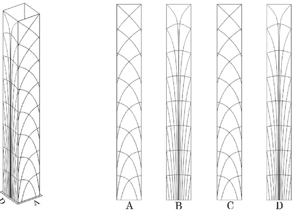
To better understand that force flow behaviour other wind load action angles have been adopted, 22.5°, 45°, 67.5° and 90°, and due to the double symmetry of the cross section the other impact angle responses should be deduced by analogy. The principal stresses trajectories are listed as in the previous angles list:

(55)

37 Figure 5.7 Principal stress trajectories for 3D cantilever problem at impact angle 22.5°

(56)

38 Figure 5.9 Principal stress trajectories for 3D cantilever problem at impact angle 67.5°

(57)

39 As should be observed, since the 0° case, there is a strip in the façade where the force “enters” somehow into the structure and propagate its stresses like vanes into the body. Just moving this entry point the same scheme rotates around the surface maintaining the same topology. This behaviour is even more clear if we observe the same load case to a cantilever tube of circular cross section.

The curves for the given problem have been drawn by a MatLab code, which is programmed for a cantilever tube with rectangular cross section under a transversal distributed load. The code and its features are presented in the appendix at the end.

5.3.

The shear-lag effect on stress distribution and principal trajectories

. In our case, having a thin closed cross section, the shear-lag effect should play a relevant role and the hypothesis where sections remain plane after deformation is far from the real behaviour of this kind of structure. Following the theories of Eric Reissner [46] in his paper, the real normal stress trend, particularly into flanges, is not linear or constant, but follows a quadratic behaviour, focussing higher amount of stresses into corners than in the centre of the side. Having the same moment in the section, but with a different stress redistribution the corners elements suffer a higher effect given by loads, and this phenomenon it was called shear-lag.

Moreover, it was observed by Foutch and Chang in 1982 [12] an anomaly in the shar-lag redistribution also, for box cantilever beam, because after the fourth quarter of the beam, the previous stress trend inverted its behaviour. This last phenomenon is then called negative shear-lag.

(58)

40 Figure 5.11 Bold lines represent shear-lag distribution and the dotted line the Eulerian stresses distribution. The case a) is for sections close to the clamped edge, so in typical shear-lag, while the case b) is close to the free edge, so in negative shear-lag

Then, the overall stresses distribution in a general cross-section becomes:

Figure 5.12 Section stress state for 3D square section cantilever problem under orthogonal uniform distributed transversal load, normal stress σz with shear-lag effect (right) and shear

stress τxz and τyz (left) which remain invariant

For more information on this effect is suggested to refer to the Reissner papers [13] and Fouth at all [12], or to check the appendix.

This different stress distribution affects the principal stresses trajectories and a new set of curves is then draw basing on previous approach, and later compared with the set without shear-lag. For this comparison only the load case indicated with 0° impact angle is taken into account.

(59)

41 Figure 5.13 Principal stresses trajectories for 3D cantilever problem at impact angle 0° and shear-lag effect

The most evident aspect is the dominant behaviour of the shear when the normal stresses take this new trend, in particular, the 45° layout becomes dominant quite immediate in the second half of the cantilever.

More considerations on shar-lag and its layout will be given in the last chapter with some numerical example and in the appendix for the theoretical demonstration.

(60)

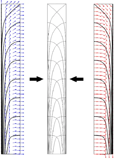
42 Figure 5.14 Principal stresses trajectories for impact angle 0°. Case a) webs for no shear-lag (left) and shear-lag (right), case b) flanges for no shear-lag (left) and shear-lag (right)

(61)

Now that we have an overall view of the problem, a comparison between optimization methods to find the optimal layout is presented and later an approach for the multiload case is implemented