Sparse computations on GPGPUs

(1)

Sparse Computations on GPGPUs

∗

Davide Barbieri

Dipartimento di Informatica, Sistemi e Produzione Universit`a di Roma “Tor Vergata”, Roma, Italy

samuelmurdoch@gmail.com

Valeria Cardellini

Dipartimento di Informatica, Sistemi e Produzione Universit`a di Roma “Tor Vergata”, Roma, Italy

cardellini@ing.uniroma2.it

Salvatore Filippone

Dipartimento di Ingegneria Industriale Universit`a di Roma “Tor Vergata”, Roma, Italy

salvatore.filippone@uniroma2.it

Universit`a di Roma “Tor Vergata”

Dipartimento di Informatica, Sistemi e Produzione

Technical Report RR-12.90

January 12, 2012

Abstract

Sparse matrix computations are ubiquitous in scientific computing; General-Purpose computing on Graphics Processing Units (GPGPU) is fast becoming a key component of high performance computing systems. It is therefore natural that a substantial amount of effort has been devoted to implementing sparse matrix computations on GPUs.

In this paper, we discuss our work in this field, starting with the data structures we have employed to implement common operations, together with the software architecture we have devised to allow interoperability with existing software packages. To test the effectiveness of our approach we have run experiments with it on two platforms; the experimental results show that our data structures allow us to achieve very good performance results, significantly better than what can be obtained with the most recent version of the CUSPARSE library.

1 Introduction

Graphics Processing Units (GPUs) have steadily entered as an attractive choice the world of scientific computing, building the core of the most advanced supercomputers and even being offered as an infrastructure service in Cloud computing (e.g., Amazon EC2). The GPU cards produced by NVIDIA are today among the most popular computing platforms; their architectural model is based on a scalable array of multi-threaded streaming multi-processors, each composed by a fixed number of scalar processors, one dual-issue instruction fetch unit, one on-chip fast memory with a configurable partitioning of shared memory and L1 cache plus additional special-function hardware. Each multi-processor is capable of creating and executing concurrent threads in a completely autonomous way, with no scheduling overhead, thanks to the hardware support for thread synchronization.

NVIDIA’s CUDA is a programming model designed for the data-parallel processing capabilities of NVIDIA GPUs [14, 19]. A CUDA program consists of a host program that runs on the CPU host, and a kernel program that executes on the GPU itself. The host program typically sets up the data and transfers it to and from the GPU, while the kernel program processes that data. The CUDA programming environment specifies a set of facilities to create, identify, and synchronize the various threads involved in the computation.

In addition to the primary use of GPUs in accelerating graphics rendering operations, there has been considerable interest in exploiting GPUs for General Purpose computation (GPGPU) [12]. A large variety of complex algorithms

∗_{This Technical Report has been issued as a Research Report for early dissemination of its contents. No part of its text nor any illustration can}

(2)

can indeed exploit the GPU platform and gain tremendous performance benefits (e.g., [10, 1, 21]). With their advanced SIMD architectures, GPUs appear also ideal candidates for performing fast operations on sparse matrices, such as the matrix-vector multiplication; this is an essential kernel in engineering and scientific computing and hence over the last two decades its efficient implementation on general-purpose architectures has been addressed in a significant amount of work. Its importance stems from the fact that a matrix-vector product is the central computational step in the execution of the most commonly used iterative solvers for linear equations, i.e., solvers based on the so called Krylov subspace projection methods [18].

Matrix-vector multiplication on GPUs presents some new challenges, because optimization techniques applied in general-purpose architectures cannot be directly applied on them. Moreover, sparse matrix structures introduce additional challenges with respect to their dense counterparts, because operations on them are typically much less regular in their access patterns. Therefore, in the last two years there has been a surge of interest about the efficient implementation of sparse matrix-vector multiplication, e.g., [3, 4, 5, 13, 17, 20], NVIDIA’s CUDPP [15].

In this paper, we consider the sparse matrix-vector multiply (SpMV) operation y ← αAx + βy where A is large and sparse and x and y are column vectors. The storage format used for the matrix A is a crucial factor in determining the performance of sparse matrix computations.

To address this issue, we have designed and developed a GPU-friendly storage format for sparse matrices and we have integrated it in our software libraries [8, 6] to extend the support provided by the GPU platform. The GPU-friendly storage format we propose is a variant of the standard ELLPACK (or ELL) format, which was previously designed for vector architectures, and is therefore named as ELLG. To test the effectiveness of our approach, we have run experiments with it on two different platforms, a desktop machine and a cluster, and we have compared the performance attained by our ELLG format to that of the CSR storage format of the CUDA CUSPARSE library, wrapping both the GPU side kernels in an existing library for parallel sparse applications. Our results show that the proposed ELLG format outperforms the CSR storage format of CUSPARSE.

The remaining of this paper is organized as follows. In Section 2 we present our GPU-friendly sparse matrix format. In Section 3 we describe the software architecture we have devised to allow interoperability with existing software packages. In Section 4 we discuss our experimental results. Finally, we draw some conclusions and give hints for future work in Section 5.

2 A GPU friendly sparse matrix format

According to the definition given by Wilkinson:

A matrix is sparse when there are so many non-zeros that it pays off to take advantage of them in the computer representation.

It should therefore not be surprising that the performance of sparse matrix computations depends critically on the specific representation chosen. There are multiple factors that contribute in determining the overall performance:

• the match between the data structure and the underlying computing architecture, including the possibility of

exploiting special hardware instructions;

• _{the amount of overhead due to the explicit storage of indices;}

• the amount of padding with explicit zeros that may be necessary.

Many storage formats have been invented over the years; a number of attempts have also been directed at standardizing the interface to these data formats for convenient usage (see e.g., [7]).

Three widely-used data formats for representing sparse matrices are COOrdinate (COO), Compressed Sparse Row (CSR), and Compressed Sparse Column (CSC).

The COO format is a particularly simple storage scheme. As shown in Figure 2, three arrays (Elements,Col idx, andRow idx) store the values, column indices, and row indices, respectively, of the non-zero entries.

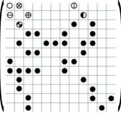
The CSR format is perhaps the most popular general-purpose sparse matrix representation. It explicitly stores column indices and non-zero values in two arrays (ElementsandCol idxin Figure 3). A third array of row pointers (Row Pointerin Figure 3) allows the CSR format to represent rows of varying length. The name is based on the fact that the row index information is compressed with respect to the COO format. Figure 3 illustrates the CSR representation of the example matrix shown in Figure 1.

(3)

Figure 1: Example of sparse matrix

Figure 2: COO compression of matrix in Figure 1

Finally, the CSC format is similar to CSR except that the matrix values are read first by column, a row index is stored for each value, and column pointers are stored.

The previous data formats can be thought of as “general-purpose”, at least to some extent, in that they can be used on most computing platforms with little changes. Additional (and somewhat esoteric) formats become necessary when moving onto special computing architectures. Many examples of these formats are available from the vector computing era, including the ELLPACK (or ELL) and Jagged Diagonals (JAD) formats. For example, the latter represents the (compressed) diagonals occurring in the matrix obtained by sorting the CSR index arrays according to their population. The main issue with vector computers was to find a good compromise between the amount of overhead and the introduction of a certain amount of “regularity” in the data structure allowing the use of vector instructions.

The situation in the case of GPUs bears both resemblances and differences: we have to accommodate for the coordinated action of multiple threads in an essentially SIMD fashion; however, we have to make sure that we have many independent threads available, the number of threads in action at any given time being much larger than the typical vector lengths of vector computers.

(4)

The ELLPACK/ITPACK format (shown in Figure 4) in its original conception comprises two 2-dimensional arrays (ElementsandCol idx) containing n ∗ kmaxelements, where n is the number of rows and kmaxis the maximum

number of non-zeros on the same row [11]. The rows of these arrays contain:

• the non-zero elements (inElements) ;

• _{their respective column indices (in}_{Col idx);}

• _{padding with zeros, where necessary.}

Figure 4: ELLPACK compression of matrix in Figure 1

For our CUDA implementation, we searched for the matrix format that allows to reach the maximum performance of one of the most frequent building blocks in linear algebra’s applications, that is the sparse matrix-vector multiply routine. Sparse matrix-vector multiply is a data-parallel routine of course, but it is memory-bounded anyway, since we have a little amount (in CUDA scale) of floating point operations per memory access, and we cannot provide an efficient memory access pattern on GPU to both sparse matrix and input vectors. Therefore, our solution was to adapt the ELLPACK format to a GPU implementation, since it provides a straightforward way to read the sparse matrix values and one of the input vectors in a efficient manner (i.e., using coalesced accesses on NVIDIA GPUs), provided that we choose a pitch for arrays that makes them aligned to the appropriate boundaries in memory (128B is a good choice for all compute capabilities). This is possible if every thread computes one of the resulting elements, and thus reads a whole compressed row (assuming a column-major order). To deal with the different number of non-zero elements per row, a simple solution is to introduce padding (elements equal to zero) to fill unused locations of the elements array. An even better solution is to create an additional array of row lengths, at the cost of just one more access per row; this is similar to CSR storage, except that we are keeping the regular memory occupancy per row implied by the usage of 2-dimensional arrays. We found that other groups have used a similar solution, e.g., in the ELLPACK-R format described in [20].

The code that uses the format is listed below:

{ y = A∗ x } p r o c e d u r e spMV ( ValuesA , I n d i c e s A , RowsDim , x , y ) i d x = t h r e a d I d x + b l o c k I d x∗ b l o c k S i z e r e s = 0 ; f o r i =0 t o RowsDim ( i d x ) b e g i n i n d = I n d i c e s A ( i , i d x ) v a l = V a l ue s A ( i , i d x ) r e s = r e s + v a l∗x [ i n d ] end y ( i d x ) = r e s end

For this code, memory accesses to array x were implemented in order to use the full L1+L2 caches hierarchy on the NVIDIA’s Fermi GPU architecture, whereas the texture cache on GPU devices with previous compute capabilities. Such implementation still approaches to inefficiency when the non-zero elements are spread to the whole row, so that

(5)

we cannot take advantage from the caching values from array x (because we have highly varying indices). Another main advantage of the integration of a non-zero elements counter array is that we know from the beginning of the main loop the length of the processing row, so we can operate programming techniques such as loop unrolling and prefetching. Listed below we report the complete kernel for the single precision spMV routine:

# d e f i n e THREAD BLOCK 128 / / O p e r a t i o n i s y = a l p h a∗Ax+b e t a ∗ y / / x and y a r e v e c t o r s / / cM i s t h e e l e m e n t s a r r a y / / rP i s t h e c ol um n p o i n t e r a r r a y / / r S i s t h e non−z e r o c o u n t a r r a y / / n i s t h e number o f r ow s g l o b a l v o i d S s p m v m g p u u n r o l l 2 k r n ( f l o a t ∗y , f l o a t a l p h a , f l o a t∗ cM , i n t ∗ rP , i n t ∗ rS , i n t n , i n t p i t c h , f l o a t ∗x , f l o a t b e t a ) { i n t i = t h r e a d I d x . x+ b l o c k I d x . x∗THREAD BLOCK; i f ( i >= n ) r e t u r n ; f l o a t y p r o d = 0 . 0 f ; i n t r o w s i z e = r S [ i ] ; r P += i ; cM += i ; f o r ( i n t j = 0 ; j < r o w s i z e / 2 ; j ++) { i n t p o i n t e r s [ 2 ] ; f l o a t v a l u e s [ 2 ] ; f l o a t f e t c h e s [ 2 ] ; / / P r e f e t c h i n g p o i n t e r s and v e c t o r v a l u e s p o i n t e r s [ 0 ] = r P [ 0 ] ; f e t c h e s [ 0 ] = t e x 1 D f e t c h ( x t e x , p o i n t e r s [ 0 ] ) ; p o i n t e r s [ 1 ] = r P [ p i t c h ] ; f e t c h e s [ 1 ] = t e x 1 D f e t c h ( x t e x , p o i n t e r s [ 1 ] ) ; v a l u e s [ 0 ] = cM [ 0 ] ; v a l u e s [ 1 ] = cM[ p i t c h ] ; cM += 2∗ p i t c h ; r P += 2∗ p i t c h ; y p r o d += f m u l r n ( v a l u e s [ 0 ] , f e t c h e s [ 0 ] ) ; y p r o d += f m u l r n ( v a l u e s [ 1 ] , f e t c h e s [ 1 ] ) ; } / / odd row s i z e i f ( r o w s i z e % 2 ) { i n t p o i n t e r = r P [ 0 ] ; f l o a t f e t c h = t e x 1 D f e t c h ( x t e x , p o i n t e r ) ; f l o a t v a l u e = cM [ 0 ] ; y p r o d += f m u l r n ( v a l u e , f e t c h ) ; } i f ( b e t a == 0 . 0 f ) y [ i ] = ( a l p h a ∗ y p r o d ) ; e l s e

(6)

y [ i ] = f m u l r n ( b e t a , y [ i ] ) + f m u l r n ( a l p h a , y p r o d ) ;

}

3 Interfacing with library code

The usage of sparse matrix packages has always been a major issue confronting both the user community and the software designers.

Ideally, each new data storage should be simply pluggable into an existing software framework without any undue effort. This has been obtained by embedding the GPU side data structures in an existing framework based on the Fortran 2003 language.

The basic ideas of the embedding are as follows:

• _{each sparse matrix has a dual representation, in main memory as well as in the GPU device memory;}

• the sparse matrix is usually built in an incremental manner on the CPU side; it is only at the finalization step

that the resulting data structure is copied on the GPU device memory;

• the sparse matrix is layered according to the “STATE” design pattern [9], with an outer shell and an inner object

whose dynamic type can change to accommodate the needs of the application.

A more detailed discussion of the interfacing issues may be found in [2]. This scheme has also been replicated by devising an interface to the sparse matrix structure available in the CUSPARSE library from the CUDA development toolkit version 4.0 [16]; the principle is the same, but the details are slightly different since the CUDA matrix is based on the CSR storage format.

The major issue in interfacing the inner data structures is the need to avoid as much as possible data movement between the host main memory and the GPU device memory (e.g., see [22]); each data movement entails a substantial overhead that, for the kind of operations we are considering, is capable of overcoming any performance advantage accrued by using the GPU device. This is achieved for the sparse matrix data structures by copying them from main memory to the GPU memory at the time of assembly (i.e., when the storage representation is fixed at the end of the coefficient build loop); the appropriate data structure is passed to the assembly code via a “mold” variable, according to the “prototype” design pattern [9].

do i = 1 , n i f ( < t h i s i n d e x b e l o n g s t o me> ) t h e n nz = <number o f e n t r i e s i n e q u a t i o n i > i a ( 1 : nz ) = i j a ( 1 : nz ) = < l i s t o f n e i g h b o u r s o f i > v a l ( 1 : nz ) = < c o e f f i c i e n t s A i j > c a l l s p i n s ( nz , i a , j a , v a l , a , d e s c a , i n f o ) e n d i f enddo c a l l s p a s b ( a , d e s c a , i n f o , mold= a e l l g )

A similar strategy has been also applied for the vectors involved in the matrix-vector product and in the other operations typical of the sparse linear system solvers commonly in use. Each vector object has two images, one in main memory and one in the GPU memory. Whenever an operation is invoked that involves these objects, the code keeps track of whether the GPU memory holds an up-to-date copy of the data; operations on the vectors are executed preferentially on the GPU side, and the GPU acts as a sort of “magnet” in that the data remains there until the user explicitly requires a synchronization with the CPU main memory (e.g., by requesting a copy to a normal array). Thus, we have a kind of “on demand” placement of data that acts in a completely transparent manner, without changing the linear solver code. The relevant methods are theis_host()method which signals that the up-to-date copy of the vector is in the host memory, theset_dev()method which signals that an operation occurred such that the up-to-date copy is the one on the device side, and thesync()method which copies the host image onto the device, or viceversa, as necessary to make sure the two copies of the data are synchronized.

(7)

s u b r o u t i n e d e l g v e c t m v ( a l p h a , a , x , b e t a , & & y , i n f o , t r a n s ) u s e i s o c b i n d i n g i m p l i c i t none c l a s s ( d e l g s p a r s e m a t ) , i n t e n t ( i n ) : : a r e a l ( d p k ) , i n t e n t ( i n ) : : a l p h a , b e t a c l a s s ( d v e c t ) , i n t e n t ( i n o u t ) : : x c l a s s ( d v e c t ) , i n t e n t ( i n o u t ) : : y i n t e g e r , i n t e n t ( o u t ) : : i n f o c h a r a c t e r , o p t i o n a l , i n t e n t ( i n ) : : t r a n s i f ( x%i s h o s t ( ) ) c a l l x%s y n c ( ) i f ( b e t a / = d z e r o ) t h e n i f ( y%i s h o s t ( ) ) c a l l y%s y n c ( ) end i f i n f o = s p m v E l l D e v i c e ( a%d e v i c e M a t ,& & a l p h a , x%d e v i c e V e c t ,& & b e t a , y%d e v i c e V e c t ) c a l l y%s e t d e v ( )

With the appropriate support we can then have a sparse linear solver such as Conjugate Gradient (CG) to run unchanged on the GPU, by simply feeding the appropriate data objects:

c a l l p s b g e a x p b y ( one , b , z e r o , r , d e s c a ) c a l l psb spmm (−one , A, x , one , r , d e s c a ) r h o = z e r o i t e r a t e : do i t = 1 , i t m a x c a l l p r e c%a p p l y ( r , w , d e s c a ) r h o o l d = r h o r h o = p s b g e d o t ( r , z , d e s c a ) i f ( i t == 1 ) t h e n c a l l p s b g e a x p b y ( one , z , z e r o , p , d e s c a ) e l s e b e t a = r h o / r h o o l d c a l l p s b g e a x p b y ( one , z , b e t a , p , d e s c a ) e n d i f c a l l psb spmm ( one , A , p , z e r o , q , d e s c a ) s i g m a = p s b g e d o t ( p , q , d e s c a ) a l p h a = r h o / s i g m a c a l l p s b g e a x p b y ( a l p h a , p , one , x , d e s c a ) c a l l p s b g e a x p b y (− a l p h a , q , one , r , d e s c a ) r n 2 = p s b g e n r m 2 ( r , d e s c a ) bn2 = p s b g e n r m 2 ( b , d e s c a ) e r r = r n 2 / bn2 i f ( e r r . l t . e p s ) e x i t i t e r a t e enddo i t e r a t e c a l l x%s y n c ( )

4 Experimental results

To test the effectiveness of our approach we have selected a set of test cases and we have run experiments with it on two platforms. The first platform is a desktop machine installed at our university; it is equipped with an AMD AthlonTM_{7750 Dual-Core Processor, and an NVIDA GTX-285 graphics card. The second platform is a cluster of the}

CASPUR supercomputing center, each node of which hosts an Intel Xeon X5650, with NVIDIA Tesla C2050 graphics card. In the following, the two platforms are referred to as GTX 285 and C2050, respectively.

(8)

Card model Clock Bus speed Bus width Peak DP

GTX 285 648 MHz 159 GB/s 512 b 90 GFLOPS

C2050 575 MHz 144 GB/s 348 b 515 GFLOPS

Table 1: The GPU models employed

matrix N N Z MFLOPS Speedup

CPU xGPU GPU

pde05 125 725 414 21 55 0.13 pde10 1000 6400 723 154 481 0.67 pde20 8000 53600 794 624 3610 4.55 pde30 27000 183600 545 881 7784 14.27 pde40 64000 438400 439 791 10380 23.63 pde50 125000 860000 436 848 12452 28.54 pde60 216000 1490400 444 981 13842 31.18 pde80 512000 3545600 454 1162 15250 33.63 pde90 729000 5054400 449 1223 15354 34.20 pde100 1000000 6940000 443 1273 15664 35.35

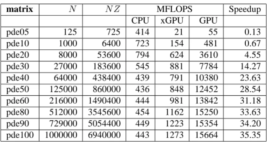
Table 2: ELLG matrix-vector product performance on platform 1 — GTX–285

On both platforms we have compiled the inner GPU computational kernels with the CUDA toolkit version 4.0, whereas the outer layers were compiled with the GNU Compiler Collection 4.6.1, employing the Fortran, C and C++ drivers for various parts of the system. To position our work we have also considered the CUSPARSE library that is part of the CUDA toolkit version 4.0 [16]; it proposes a storage format that is essentially identical to the CSR format (in the following, referred to as CSRG). We have wrapped the GPU side kernels in a manner similar to our own ELLG kernels, so as to be able to use exactly the same test programs; therefore all overhead factors are the same for both sets of kernels. All experiments have been run in double precision, as this is usually necessary for the problems that are typically encountered in contemporary scientific applications.

The main features of the two graphics cards are shown in Table 1; for the interpretation of our subsequent results it is very important to look carefully at the various performance metrics. In particular, the Tesla C2050 has a much better execution rate for double precision floating point arithmetic; however, and somewhat counterintuitively, it also shows a lower clock rate and a lower bus speed. As we shall see, since our sparse computations are latency and memory bound, the peak performance indicator is not necessarily accurate, and indeed the older GTX-285 card actually does outperform the newer C2050.

Table 2 shows the performance of the matrix-vector product in MFLOPS for the first platform. The matrices have been generated from the finite difference discretization of Partial Differential Equation (PDE) on a cubic domain with a uniform step size; the name of the matrix in the first column refers to the length of the cube edge in the discrete units. The second column reports the number of rows and columns in the matrix, whereas the third column the number of non-zero elements; most rows in each matrix contain 7 non-zero elements. The column labeled CPU shows the performance of the matrix-vector product as implemented on the CPU with the CSR storage format; the column labeled xGPU is the performance with the product executed on the GPU but including the overhead of transferring the x and y vectors from main memory to the device; the GPU column shows the performance data when the x and

y vectors are in the GPU memory from the beginning, and finally we also list a speedup of the GPU vs the CPU

computation. The measurements were obtained by performing 2000 products in sequence, and computing the overall execution rate. Table 3 is built in exactly the same way, but the data have been gathered on the second platform.

As we can see, in both cases for the CPU column there is a surge in performance at low to medium sizes, then followed by a levelling off for large matrix cases; this is due to the memory occupation of the matrix overflowing the cache memory, which is larger for platform 2. Performing the matrix-vector products in a sequence, with a warm cache, is consistent with the usage within the iterative linear system solvers which are our target applications, where one or more products are performed within each iteration. The CPU performance is better for platform 2; however exactly the opposite is true for the GPU performance; since the sparse matrix-vector computation is bound by the accesses to

(9)

CPU xGPU GPU

Table 3: ELLG matrix-vector product performance on platform 2 — C2050

CPU xGPU GPU

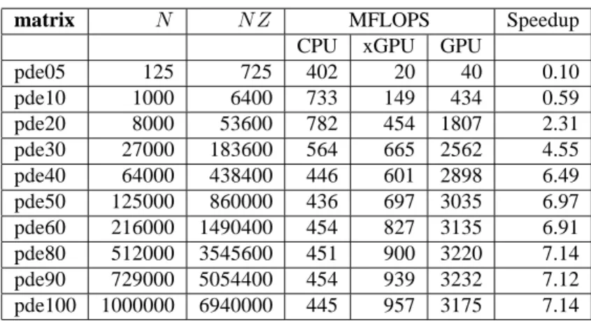
Table 4: CSRG Matrix-vector product performance on platform 1 — GTX–285

the memory subsystem, the superior floating point performance of the C2050 platform does not compensate for the higher clock rate and bus speed of the GTX-285 platform. In both cases the sparse kernel execution rate is much lower than the peak execution rate, which is known to be achievable with a good approximation when running kernels for dense matrices, such as the matrix-matrix product DGEMM.

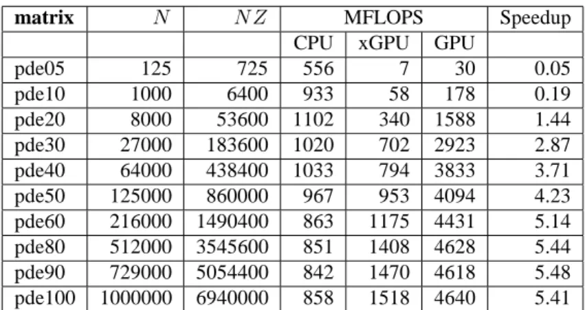
Tables 4 and 5 report the results of the same measurements, with the same program but using the data structures and inner kernels from the CUSPARSE library. As we can see, we have a very different behaviour, in that:

1. the attained GPU performance is significantly lower in both cases;

2. platform 2 (the Tesla C2050) is slightly better than platform 1 (the GTX-285).

Especially in the GTX-285 case, the regularity of memory accesses in our data structure as opposed to the more irregular accesses in memory that are intrinsic to CSR makes a large difference in the attained performance; this is still true on the C2050, albeit to a much lesser extent, since the underlying Fermi architecture is substantially different from that of the older card, and in particular it suffers much less from uncoalesced accesses to memory.

5 Conclusions

In this paper, we have discussed the implementation issues of the sparse matrix by dense vector product kernel on GPU devices, specifically on the NVIDIA GPUs. We have presented the ELLG format, which is derived from the ELLPACK format and properly adapted to a GPU implementation, and described how the proposed data storage can be simply plugged into existing software frameworks for parallel sparse applications. We have shown that how our

(10)

CPU xGPU GPU

Table 5: CSRG Matrix-vector product performance on platform 2 — C2050

data structures allow us to achieve very good performance results, significantly better than what can be obtained with the CUSPARSE library version 4.0.

The overall software infrastructure in which this work is embedded has been described in other papers [X,Y], and is an ongoing effort. Since the final objective is to enable applications to run on the GPU, future work will include:

• _{Further tuning of the kernels;}

• Testing in the context of a complete iterative solver;

• Studying the various possibilities for implementing suitable preconditioners for the Krylov methods;

• Exploring the possibility of interfacing our software from high-level environment such as MATLAB or Octave;

• Extending our GPU-enablement to the full MPI version of our software.

Much work lies still ahead of us; moreover, a lot of work will be needed to keep pace with the changes in the architec-tural landscape. This is very reminiscent of the situation during the various development cycles in High Performance Computing platforms, first with vector computers from the early 70s into the 90s, then with RISC machines and clusters from the late 80s onwards.

Acknowledgments

We wish to acknowledge the organization of the CASPUR supercomputing center for awarding us with a grant for access to the experimental platform 2 under the HPC-Grant 2011 program.

References

[1] D. Barbieri, V. Cardellini, and S. Filippone. Generalized GEMM applications on GPGPUs: Experiments and applications. In Proc. of 2009 Int’l Conf. on Parallel Computing, ParCo ’09. IOS Press, 2009.

[2] D. Barbieri, V. Cardellini, S. Filippone, and D. Rouson. Design Patterns for Scientific Computations. In Europar 2011, Bordeaux, France, 2011.

[3] M. M. Baskaran and R. Bordawekar. Optimizing sparse matrix-vector multiplication on GPUs. Technical Report RC24704, IBM Research, Apr. 2009.

[4] N. Bell and M. Garland. Implementing sparse matrix-vector multiplication on throughput-oriented processors. In Proc. of Int’l Conf. on High Performance Computing Networking, Storage and Analysis, SC ’09. ACM, 2009.

(11)

[5] J. W. Choi, A. Singh, and R. W. Vuduc. Model-driven autotuning of sparse matrix-vector multiply on GPUs. SIGPLAN Not., 45:115–126, Jan. 2010.

[6] P. D’Ambra, D. di Serafino, and S. Filippone. MLD2P4: a package of parallel algebraic multilevel domain decomposition preconditioners in Fortran 95. ACM Trans. Math. Softw., 37(3):7–23, Sept. 2010.

[7] I. Duff, M. Marrone, G. Radicati, and C. Vittoli. Level 3 basic linear algebra subprograms for sparse matrices: a user level interface. ACM Trans. Math. Softw., 23(3):379–401, Sept. 1997.

[8] S. Filippone and M. Colajanni. PSBLAS: a library for parallel linear algebra computations on sparse matrices. ACM Trans. on Math Software, 26:527–550, 2000.

[9] E. Gamma, R. Helm, R. Johnson, and J. Vlissides. Design Patterns: Elements of Reusable Object-Oriented Software. Addison-Wesley, 1995.

[10] W.-M. Hwu. GPU computing gems emerald edition. Morgan Kaufmann, first edition, 2011.

[11] D. R. Kincaid, T. C. Oppe, and D. M. Young. ITPACKV 2D Users Guide. http://rene.ma.utexas. edu/CNA/ITPACK/manuals/userv2d/.

[12] D. Luebke, M. Harris, N. Govindaraju, A. Lefohn, M. Houston, J. Owens, M. Segal, M. Papakipos, and I. Buck. GPGPU: general-purpose computation on graphics hardware. In Proc. of 2006 ACM/IEEE Conf. on Supercom-puting, SC ’06. ACM, 2006.

[13] A. Monakov, A. Lokhmotov, and A. Avetisyan. Automatically tuning sparse matrix-vector multiplication for GPU architectures. In High Performance Embedded Architectures and Compilers, volume 5952 of LNCS, pages 111–125. Springer, 2010.

[14] J. Nickolls, I. Buck, M. Garland, and K. Skadron. Scalable parallel programming with CUDA. Queue, 6:40–53, March 2008.

[15] NVIDIA Corp. CUDPP: CUDA data parallel primitives library. http://gpgpu.org/developer/ cudpp/.

[16] NVIDIA Corp. CUDA CUSPARSE library version 4.0, 2011.http://developer.download.nvidia. com/compute/cuda/4_0_rc2/toolkit/docs/CUSPARSE_Library.pdf.

[17] J. C. Pichel, F. F. Rivera, M. Fern´andez, and A. Rodr´ıguez. Optimization of sparse matrix-vector multiplication using reordering techniques on GPUs. Microprocessors and Microsystems, In Press, 2011.

[18] Y. Saad. Iterative methods for sparse linear systems. Society for Industrial and Applied Mathematics, Philadel-phia, PA, second edition, 2003.

[19] J. Sanders and E. Kandrot. CUDA by example: An introduction to general-purpose GPU programming. Addison-Wesley, first edition, 2010.

[20] F. Vazquez, G. Ortega, J. J. Fern´andez, and E. M. Garzon. Improving the performance of the sparse matrix vector product with GPUs. In Proc. of 10th IEEE Int’l Conf. on Computer and Information Technology, pages 1146–1151, 2010.

[21] V. Volkov and J. W. Demmel. Benchmarking GPUs to tune dense linear algebra. In Proc. of 2008 ACM/IEEE Conf. on Supercomputing, SC ’08. IEEE Press, 2008.

[22] R. Vuduc, A. Chandramowlishwaran, J. W. Choi, M. E. Guney, and A. Shringarpure. On the limits of GPU acceleration. In Proc. of 2nd USENIX Workshop on Hot Topics in Parallelism (HotPar ’10), June 2010.