Neural networks algorithms for the estimation of atmospheric ozone from Envisat-SCIAMACHY and Aura-OMI measurements

(1)

TOR VERGATA UNIVERSITY, ROME, ITALY

Department of Computer, Systems and Industrial Engineering

GeoInformation PhD Programme XXI Cycle

Neural Networks algorithms for the

estimation of atmospheric ozone from

Envisat-SCIAMACHY and Aura-OMI

measurements

A thesis submitted in partial fulfillment for the degree of Doctor of Philosophy

Mentor: Fabio Del Frate Candidate: Pasquale Sellitto

(2)

Dedicated to Chiara

(3)

“Nature - the Gentlest Mother is Impatient of no Child

The feeblest or the waywardest Her Admonition mild

In Forest and the Hill By Traveller be heard Restraining Rampant Squirrel Or too impetuous Bird

How fair Her Conversation A Summer Afternoon

Her Household Her Assembly And when the Sun go down

-Her Voice among the Aisles Incite the timid prayer Of the minutest Cricket The most unworthy Flower

When all the Children sleep -She turns as long away

As will suffice to light Her lamps Then bending from the Sky

With infinite Affection And infiniter Care

Her Golden finger on Her lip -Wills Silence - Everywhere -”

(4)

Acknowledgements

Nel settembre 2005, da neolaureato in Fisica all’Università “La Sapienza”, decisi di partecipare all’esame di ammisione al corso di Dottorato di Ricerca in GeoInformazione, all’Università “Tor Vergata”, Dipartimento di Ingegneria dell’Informazione. Oggi posso ammetterlo, avevo letto, in fretta e furia solo 2 o 3 articoli sul telerilevamento dell’atmosfera da satellite, li avevo letti rapidamente e non ci avevo capito molto. Ero vestito da “fisico”, il che scatenó qualche ilarità1, e non conoscevo nessuno a Tor Vergata. Avevo alle spalle un contratto (che avevo rifiutato) da studente di dottorato al Forschungszentrum Jülich e la ragionevole prospettiva di vincere una posizione analoga per il dottorato in Teler-ilevamento a “La Sapienza”. Invece vinsi qui, anche grazie alle rinunce di Cosimo e Alessandro, e decisi di accettare. Vinsi anche grazie a due parole che avevo letto dis-trattamente su uno dei 2 o 3 famosi articoli. Un membro della commisione esaminatrice mi chiese come mi aspettavo si potesse ricavare un profilo di qualcosa da uno spettro di qualcosa. Il membro era il Prof. Fabio Del Frate, la risposta fu Optimal Estimation. Un guizzo di memoria ed ecco la risposta. Non sapevo esattamente di cosa stessi parlando, ma la risposta era giusta e l’avevo data grazie a 2 articoli a caso letti pochi minuti prima. Dunque avevo cambiato al contempo Facoltà e Ateneo, ero un dottorando a “Tor Ver-gata” per merito di un caso fortunato e di due rinunce. Oggi ripenso a quel giorno come una svolta fondamentale della mia vita, che mi aveva aperto le porte a una esperienza non sempre facile, a volte frustrante, ma che, come poche altre, mi ha instradato verso il mio futuro. Per questo il mio primo ringraziamento va al Caso, al Destino, a Dio, come vogliamo chiamare il motore di questi eventi.

Tre anni duri ma con un altissimo coefficiente di crescita personale, dicevo. Per questo vorrei ringraziare fortemente il Prof. Fabio Del Frate, che ha permesso e favorito lo sviluppo delle mie capacit`a di (nascente) ricercatore, e che, grazie alla sua grande pacatezza, ha consentito una crescita “indipendente”. Allo stesso modo vorrei ringraziare il Prof. Domenico Solimini, e lo staff del programma di dottorato in GeoInformazione. Un ringraziamento al Prof. Pawan K. Bhartia del NASA-GSFC per la sua disponibilit`a durante il mio periodo di ricerca in America, e a tutto l’Atmospheric Chemistry and Dynamics Branch del NASA-GSFC. In questo contesto voglio fare un ringraziamento speciale a Christian Retscher (che anche autore del Paragrafo (2.2.6)) e Bojan Bojkov dell’AVDC per il loro competente supporto.

Un ringraziamento a tutti gli studenti di dottorato dell’EOLab (in senso antiorario a partire dalla mia postazione in laboratorio), Giorgio Licciardi, Fabio Pacifici, Chiara Pratola, Michele Lazzarini, Emanuele Angiuli, e agli ex-studenti e a quelli che non sono

1

E’ ben noto come gli Ingegneri facciano una grande attenzione all’abbigliamento, il che li porta spesso e volentieri a indossare dei gilet grigi.

(5)

stati fisicamente nell’EOLab, Andrea Minchella (a cui aggiungo un ringraziamento per il supporto all’Envisat Symposium 2007), Andrea Radius, Chiara Solimini, Riccardo Duca, Alessandro Burini, Cosimo Putignano, e tutti gli altri. Un ringraziamento a Michele Iapaolo per avermi aiutato nelle prime fasi del mio dottorato.

Infine un grande ringraziamento a tutti i miei amici e familiari, senza i quali non avrei raggiunto questo n´e alcun altro obiettivo, ai miei genitori, a mio fratello Luca, a Chiara, mia moglie, che ha mi supportato e sopportato in questi anni. Il contributo di Chiara a questo traguardo incalcolabile e a lei dedico la mia tesi.

I acknowledge Dr. Christian Retscher for the contents of Sec. (2.2.6). I’d like to acknowledge the owners and providers of WOUDC and SHADOZ ozonesondes data. Eng. Emanuele Angiuli is gratefully acknowledged for his valuable IDL advices. Eng. Alessandro Burini is acknowledged for the fruitful collaboration and discussion regarding the dataset preparation for the work described in Chapter (5). Dr. Mark Kroon from KNMI is acknowledged for his highly skilled management of OMI cal/val AO, including project no. 2930.

(a) Tipiche condizioni meteo a Greenbelt, MD, USA

(b) IV giornata della GeoInformazione, Marzo 2006: molta eleganza sprecata

(c) Poich´e la mensa dell’Universit`a non soddisfa i dottorandi, tre di loro vanno a pranzo a Frascati

(d) Me medesimo in abbondanza di scattering molecolare

(6)

(7)

Summary

Climate changes and atmospheric pollution are currently topical issues given their possi-ble dramatic effects from the health, social and economical points of view. Assessing the causes and possible adaptation/mitigation strategies is a challenge in modern science. To understand and quantify the anthropic role in such changes is of a particular interest to depict future scenarios and to warn politicians about local and global intervention in emissions control.

Ozone is one of the most important trace gases in the Earth’s atmosphere. It is mainly present in the stratosphere, with only 10% in the troposphere. Despite its small amount, (2-7)·10−3 % in molar fraction, the solar radiation at wavelengths below 310 nm does not reach the Earth surface because of the large absorption cross sections characterizing ozone molecules at those wavelengths. Variations in the stratospheric ozone content may play a dramatic role in a possible increase of the surface UV radiation. The discovery of the Antarctic ozone hole, i.e. a considerable reduction of ozone in the polar stratosphere, was a dramatic evidence of the effects of anthropogenic emissions on the ozone layer. Human activity is likely responsible also for tropospheric ozone enhancements caused by the photochemistry associated to industrial emissions involving ozone precursors as the nitrogen dioxide. The effect of these variations at lower altitudes, with respect to background values, have been estimated to be the third largest source of the greenhouse effect.

To support interpretation of the atmospheric phenomena, as well as interactions with the oceans and the ground, a constant and systematic monitoring of several atmospheric parameters, and with a good spatial coverage, is crucial. In this framework, global and systematic space-based observations of the atmospheric composition and its variations in time and space play a major role. Satellite measurements of atmospheric parameters has a proven and recognized effectiveness for such tasks. The advantage of atmospheric sounding performed from space, with respect to ground based techniques, lies in the very high number of available measurements per day and in the global coverage of the Earth, allowing for a detailed and continuous investigation of the atmospheric state.

(11)

Summary 2

A number of different techniques are available , using different instruments, bands and viewing geometries. For all of them, a major problem is related to the intrinsically indirect nature of the measurements, as they result from the interaction between the electromagnetic radiation and the atmospheric constituents. The retrieval phase requires the solution of an inverse problem, which is never trivial and can be computationally very intensive, especially for this kind of nonlinear problems. A significant concurrent requirement is an adequate spatial resolution. Horizontal resolution is very hard to achieve by limb measurements, while it can be attained by nadir observations. Nadir measurements, however, can have poor vertical resolutions, and the inversion problem can be particularly computationally expensive.

In this thesis we present novel approaches to the inversion of the nadir UV/VIS satel-lite Earth’s radiance spectra for the retrieval of height resolved ozone information. The considered platforms are ESA EnviSat-SCIAMACHY and NASA-Aura OMI, which are particularly suited for these tasks owing to their combined high spectral and spatial res-olutions. Both ozone concentration profiles and tropospheric ozone column are retrieved by means of NNs algorithms. NNs are made of interconnected elementary processing units, called neurons, and can learn from a training dataset; they were proven to be robust on systematic errors and calibration uncertainties on the input measurements vector, and they are likely to work better than OE with respect to cloudy scenarios or in presence of significant aerosols burdens. Once a net is trained it can perform retrievals in real-time.

The work has been fulfilled in the framework of the GeoInformation PhD Programme of Tor Vergata University of Rome, and with the NASA - Goddard Space Flight Center in Greenbelt, MD, USA.

(12)

Chapter 1

Atmospheric ozone measurements

1.1 Atmospheric structure and composition

The Earth’s atmosphere is the layer of gases and suspended solid and liquid particles surrounding the planet Earth; it is retained by Earth’s gravity. Table 1.1 summarizes the molar fraction of major atmospheric gasses.

As it is possible to notice, over the 99% of the mass of the atmosphere is composed by the N2 and the O2. Although representing, collectively, only the ∼ 1% of the atmospheric

mass, some of the so-called trace gases have a major role in thermodynamical, chemical and radiative phenomenology of the Earth’s atmosphere. Other important atmospheric constituents are the aerosols, microscopic (10−3 − 102_{µm) liquid and solid particles}

suspended in the air that can absorb and/or scatter solar and terrestrial radiation within various spectral bands; the high-degree variation in time and space of their optical and

Gas Molar fraction (%) N2 78.08 O2 20.95 A 0.93 CO2 0.03 Ne 0.00182 He 0.00052 CH4 0.00015 Kr 0.00012 H2 0.00005 NO2 0.00005 O3 (2-7)·10−3 H2O (0-4)·10−3

Table 1.1: Atmospheric composition: molar fraction of the major atmospheric gasses [1].

(13)

Chapter 1. Atmospheric Ozone Measurements 4

morphological properties can cause a significant uncertainty to the climatic system and the Earth’s energy balance [1].

Atmospheric constituents can absorb or scatter solar and terrestrial radiation. In these processes, energy can be stored in the atmosphere and then re-emitted as IR radiation. All these phenomena, in conjunction with surface and ocean interaction with radiation, take place to maintain a radiative balance between incoming and outgoing energy in dependence of which the Earth climatic system is relatively stable.

Interacting radiative, dynamical and chemical processes determine the structure of the atmosphere. The atmosphere can be divided into several different vertical layers pos-sessing very distinct chemical, physical and dynamical properties. The primary way to display this structure is to look at the average temperature profile of the atmosphere. It is possible to identify regions in which the vertical temperature gradient has the same sign. Between layers with opposite vertical temperature gradients, it is possible to iden-tify pauses in which the gradient is approximately zero. Layers and pauses of the Earth atmosphere are enumerated and their properties briefly described in the following:

• Troposphere - The vertical temperature gradient is negative and its magnitude is ∼ 5 K/km on average [2]. Atmospheric circulation is dominated by thermal and mechanical exchanges with the surface. Convection of warmer air from lower levels is the main phenomenon for temperature control, while IR absorption/emission of some gases as well as air masses dynamics and water phase changes may have a role in the energy balance. Within the troposphere most of the atmospheric mass can be found and here meteorological phenomena occur. The troposphere is ∼ 10 km deep on average; it is deeper at the tropics, where can reach the altitude of ∼ 20 km, and shallower at the poles, where can be as low as ∼ 7 km. Its height also depends on the season.

• Tropopause - The vertical temperature gradient goes to zero and slowly changes sign. Here the temperature is relatively low, ∼ 190 − 230 K on average [2] and condensation of water vapor is favored, generally preventing this species from diffusing upwards. The troposphere height can vary depending on the variations of thickness of the troposphere.

• Stratosphere - The vertical temperature gradient is positive and its magnitude is ∼ 2 K/km on average [2]. The stratification of the air masses prevent their vertical motion. Absorption of UV radiation by the ozone is the main phenomenon for temperature control and energy balance, if we neglect heath transport due to the (mainly horizontal) air masses motion. Starting from the tropopause, the stratosphere can reach altitudes as high as ∼ 55 km.

(14)

Figure 1.1: Standard thermal structure of the atmosphere at different latitudes and

seasons. Elaborated from data taken from [3].

• Stratopause - The vertical temperature gradient goes to zero and then changes sign.

• Mesosphere - The vertical temperature gradient is negative. The UV absorption is relatively weak owing to lower gas concentrations. Starting from the stratopause, this layer can reach altitudes of ∼ 90 km [2].

• Mesopause - The vertical temperature gradient goes to zero and then changes sign. • Termosphere - The vertical gradient is positive and temperatures can reach values as high as 1000−2000 K [2]. Even if the gasses concentrations rapidly decrease with height, the absorption of UV radiation increase for the dissociation of the oxygen molecule, leading to dramatically high temperatures. In this area the atmosphere has a quasi-isothermal behavior and the species tend to stratify depending on their atomic/molecular masses.

(15)

1.2 Ozone in the Earth’s atmosphere

1.2.1 Introduction

Ozone (O3) is an allotrope of oxygen; it is mainly produced in stratosphere, from

reac-tions involving the absorption of relatively high energy solar UV radiation. Atmospheric ozone has a recognized key-role in absorbing the harmful solar UV photons at short wavelengths, and its vertical distribution affects significantly the chemical and physical processes in a large part of the atmosphere. Despite the small amount of ozone in the Earth’s atmosphere, the solar radiation at wavelengths below 310 nm does not reach the lower atmospheric layers because of the large absorption cross sections of the ozone at those wavelengths (see Sec. (1.2.4)). In this way the ozone layer acts as a filter for the harmful UV solar radiation and contributes to the radiative balance of the strato-sphere and the upper tropostrato-sphere. Although its presence in stratostrato-sphere is of a crucial importance for life on Earth, an enhancement of ozone in the troposphere may be a danger for human beings, for animals and vegetation. The ozone is highly reactive with several molecules and it can reduce human lungs capacity, worsen pre-existing cardiac and pulmonary pathologies and it can interact with crop and vegetation growing. In addition, the ozone plays a fundamental role in the tropospheric radiative balance: tro-pospheric ozone is a direct greenhouse gas [1] and it is considered to be the third most important gas in global warming, in terms of radiative forcing, after the carbon dioxide and methane [1]. Furthermore, tropospheric ozone is a source for the hydroxyl radi-cal, which controls the abundance and distribution of many atmospheric constituents, including greenhouse gases [4].

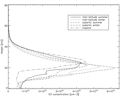
An average vertical concentration profile of ozone is reported in figure1.2. As it is pos-sible to notice, about 90% of the total ozone is in the stratosphere, while the remaining 10% is in troposphere. Ozone profiles at different latitudes and seasons are shown in figure1.3.

In the past few decades the public concern regarding the impact of human activities on the Earth’s atmosphere has significantly grown, and a considerable effort has been made by researchers in order to understand the role of anthropogenic gas emissions in the atmospheric chemistry and its connections with the stratospheric ozone depletion, the global climate change and the increasing pollution of the troposphere. Ozone studies are of a particular interest for the understanding of both surface UV flux increase and the global warming. Efforts for a more complete depiction of ozone dynamics both in the stratosphere and in the troposphere are crucial to address the human impact on climate and to monitor the effects of possible intervention for mitigation. Long-term systematic observations of height resolved ozone concentrations from satellite platform may help

(16)

Figure 1.2: A standard ozone profile at mid-latitudes. Figure taken from [5]

Figure 1.3: Standard ozone concentration profiles at different latitudes and seasons.

(17)

in this context. In Sec. (1.4) a general state of the art of this kind of measurement approach is given, and in Subsec.s (1.4.4.4) and (1.4.4.5) a specific description of existing techniques of satellite monitoring of ozone from nadir UV/VIS measurement is reported, as well as their advantages and weaknesses over other techniques. In the next few Sec.s we will briefly discussion ozone sources and sinks in both stratosphere and troposphere, and a spectroscopic characterization of this important trace gas.

1.2.2 Stratospheric ozone

1.2.2.1 Formation and removal mechanisms

Ozone concentrations in atmosphere are determined by the balance of formation, de-struction and transport.

The ozone production in stratosphere is mainly due to the photo-dissociation of oxygen molecules triggered by the incidence of UV radiation at λ < 242 nm:

O₂+ hν −−→ 2 O(3P) if λ < 242 nm (R 1.1) O₂+ hν −−→ O(3P) + O(1D) if λ < 175 nm (R 1.2)

The oxygen atoms react rapidly with the oxygen molecules to form ozone. For this reaction a third body species M is required to acquire the kinetic energy in excess:

O + O₂+ M −−→ O₃+ M + 24 kcal/mol (R 1.3)

In absence of M, an unstable vibrational state of O3 is formed, and rapidly dissociate.

In any case, O3 can dissociate by absorbing UV radiation and then it can react with the

atomic oxygen as in Reac.s (R 1.4) and (R 1.5).

O₃+ hν −−→ O + O₂ if 240 nm < λ < 320 nm (R 1.4) O₃+ O −−→ 2 O₂+ 94 kcal/mol (R 1.5)

The atomic oxygen can also re-combine to produce molecular oxygen in the following way:

(18)

Reac.s (R 1.1-R 1.6) are collectively known as the Chapman cycle and lead to a steady state, i.e. the rate of ozone loss is equal to the rate of ozone formation [6].

Additional loss cycles are attributed to highly reactive catalysts X, mainly produced in stratosphere by photolytic decomposition:

X + O₃ −−→ XO + O₂ (R 1.7) XO + O −−→ O₂+ X (R 1.8)

giving:

O + O₃ −−→ 2 O₂

Important catalysts have been identified as the HOxand NOx[7,8] or halogen species as

the Cl and the Br [7]. The OH and H gases are mainly generated by the decomposition of methane and water vapor, the NO and NO2 originate from N2O produced in the

bio-sphere, the chlorine and ClO come from industrial products as the chlorofluorocarbons (CFCs), and the bromine is generated by Halon, another industrial product.

A specific discussion on the so-called ozone hole phenomenology will be now given. Un-der normal circumstances, almost all of the chemically active (stratospheric) chlorine is in the form of HCl or ClONO2. Br compounds are much less abundant in the atmosphere

than Cl compounds, but the related loss cycles are more efficient per molecule due to the much lower fraction in (inactive) reservoir form [9]. Significant reductions in lower stratospheric O3at high latitude are well known from decades [10]. The phenomenon has

been observed in both hemispheres, and more consistently in the Antarctic. The prin-cipal cause has been identified in the enhanced release of active chlorine from reservoir species, promoted by heterogeneous multi-phase reaction on Polar Stratospheric Cloud (PSC) particles [11]. PSC formation requires the very low temperatures (< 200 K) in the polar vortex, when, in the absence of sunlight, the stratospheric air masses cool and descend, developing a circulation mechanism which produces the vortex. The core of the vortex becomes steadily isolated from the air outside and then persists until warming and mixing occurs in the spring. Reactions, including the following, occur much more readily when the second reactant on the left hand side is absorbed onto the surface of a PSC particle (denoted here by subscript (s)) [9]:

(19)

ClONO₂+ H₂O(s)−−→ HOCl + HNO3(s) (R 1.10)

HOCl + HCl(s)−−→ Cl2+ H2O (R 1.11)

The chlorine species produced in each case rapidly photolyze, given sun-light in the spring, releasing Cl which reacts with O3:

Cl + O₃−−→ ClO + O₂ (R 1.12)

Once the concentration of ClO reaches a certain level, the following cycle rapidly destroys O3:

ClO + ClO + M −−→ ClOOCl + M (R 1.13) ClOOCl + hν −−→ ClOO + Cl (R 1.14) ClOO + M −−→ Cl + O₂ (R 1.15) (2×) Cl + O₃−−→ ClO + O₂ (R 1.16)

Reac.s (R 1.13-R 1.16), together, give:

2 O₃ −−→ 3 O₂

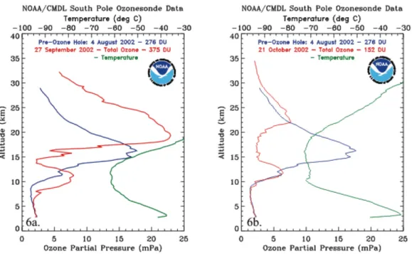
The described phenomenon brings to the mentioned ozone depletion at high latitudes, and in particular in Antarctica, which leads to a sensible reduction of ozone in the polar stratosphere and to a possible surface UV flux enhancement [7]. As an example, Fig. (1.4) shows the ozone concentration profile in a ozone hole situation. Please refer to the caption for further details.

1.2.2.2 Spatial and temporal variabilities

Here we want to discuss the average global features and the variabilities over the globe and the seasons of the total ozone. Owing to the fact that nearly the 90% of the ozone is in the stratosphere, patterns in total ozone can be representative of the stratospheric content. A further description of the tropospheric patterns and trends is given in section

1.2.3.2.

The Chapman cycle formulation of stratospheric ozone photo-chemistry leads to an expected distribution with a maximum at the equator and a minimum at the poles. The

(20)

Figure 1.4: Two ozone soundings made at the South Pole in September and October 2002 (red line), compared to a pre-ozone hole profile taken on August 2002 (blue line).

A temperature profile is also reported (green line). Figure taken from [12].

ozone production, in fact, is likely controlled by the photonic flux at sensible wavelengths, giving a maximum ozone production at lower latitudes, where the photo-chemistry is maximum due to higher illumination. The observed spatial distribution of total ozone, on the opposite, is maximum at sub-polar locations and minimum at the equator, on average [1]. A depiction of these observations is given in Fig. (1.5), where global mean total ozone for January, April, July and October 2008 is reported. Here it is also possible to see that a maximum occurs in April at about 70◦, and similarly in spring for the Southern Hemisphere.

The discrepancy between the Chapman theory and the observations is due to the fact that the theory doesn’t consider air masses circulation and transport phenomena. The maximum at higher latitudes, in fact, depends on the ozone transport from the higher stratosphere over the equatorial region, where the maximum of the ozone production can be located, to the lower and mid stratosphere over the polar region [2]. The northern high latitudes maximum is more marked than the analogous maximum in the southern hemisphere.

Finally, a closer view to the peculiar Antarctic ozone hole phenomenon is given in Fig. (1.6), where the evolution of the ozone hole in the period 1995-2004 is shown. The ozone hole is also visible in Fig. (1.5(d)).

(21)

(a) January 2008 (b) April 2008

(c) July 2008 (d) October 2008

Figure 1.5: Global mean total ozone for different months in 2008. Elaborated from data taken from [13].

Figure 1.6: The Antarctic ozone hole evolution in the period 1995-2004: September’s concentrations taken from GOME and SCIAMACHY data. Courtesy of DLR.

(22)

Figure 1.7: Scheme of the major ozone transport, formation and removal phenomena. Courtesy of NASA.

1.2.3 Tropospheric ozone

1.2.3.1 Formation and removal mechanisms

The two main sources of ozone in troposphere are Stratosphere-Troposphere Exchanges (STE), and chemical and photochemical reactions occurring in the boundary layer [14]. Figure 1.7shows a scheme of these as well as some other minor mechanisms.

In the following we will examine more thoroughly the two mentioned components.

• STE

The ozone has its major source in the mid stratosphere. Air masses can move down towards the low stratosphere by adiabatic circulation. Lower stratospheric levels, that are richer in ozone, can exchange air masses with the upper troposphere allowing the advection of ozone. An estimation of ozone flux in troposphere for STE is 360-820 Tg/year, globally [15]. STE-related transport of ozone is more effective in late winter and in spring, while the average lifetime of ozone in the free troposphere is about 1-4 months. It is expected that STE contribution to tropospheric ozone concentrations is dependent on latitude, tropopause height and season.

(23)

Another source of ozone in the troposphere is related to the photochemical activity involving CO, CH4and Volatile Organic Compounds (VOCs), in presence of nitric

oxides [16]. These species are usually referred as ozone precursors. The reactions involving CO are in the following:

CO + OH₋O₋_{→ CO}2 2+ HO2 (R 1.17) HO₂+ NO −−→ OH + NO₂ (R 1.18) NO₂+ hν O2 −−→ NO + O₃ (R 1.19) giving, at neat: CO + 2 O₂−−→ CO₂+ O₃ (R 1.20)

The contribution of CH4 is given by the following cycle:

CH₄+ OH −−→ CH₃+ H₂O (R 1.21) CH₃+ O₂+ M −−→ CH₃O₂+ M (R 1.22) CH₃O₂+ NO −−→ CH₃O + NO₂ (R 1.23) CH₃O + O₂ −−→ CH₂O + HO₂ (R 1.24) CH₂O + hν ₋O₋_{→ CHO + O}2 2 (R 1.25) CHO + O₂−−→ CO + HO₂ (R 1.26) CO + OH₋O₋_{→ CO}2 2+ HO2 (R 1.27) (4×) HO₂+ NO −−→ OH + NO₂ (R 1.28) (5×) NO₂+ hν O2 −−→ NO + O₃ (R 1.29) giving, at neat: CH₄+ 10 O₂ −−→ CO₂+ H₂O + 5 O₃+ 2 OH (R 1.30)

The VOCs can contribute in the following way:

VOC₁+ 4 O₂+ 2 hν −−→ VOC₂+ H₂O + 2 O₃ (R 1.31)

(24)

HO₂+ O₃−−→ OH + 2 O₂ (R 1.32) OH + O₃ −−→ HO₂+ O₂ (R 1.33)

The net flux of tropospheric ozone due to photochemistry has been estimated as 500-700 Tg/year [17]. The balance of Reac.s (R 1.17-R 1.33) is given by the abundance of the ozone precursors and sinks. In particular the NOx can drive

tropospheric ozone concentrations. Tropospheric NOx originates predominantly

from fossil fuel combustion . Natural sources are about of a factor 3 lower and include soil emissions and lightnings [18]. Although the NOxhave a short lifetime

(few hours near the ground, few days at higher altitude), they can be transported for large distances from localized sources, via reservoir species (e.g. peroxyacetyl-nitrate - PAN). Tropospheric convection can be important to transport the NOx

to high altitude and low temperature regions, where both NOxand PAN are more

stable [19]. Ozone production is strongly favored in urban regions under high-pressure meteorological conditions, since the vertical stability (associated with a temperature inversion) allows the primary pollutants, including NOxand

hydrocar-bons, to accumulate. Such conditions typically occur in summer, when photolysis rates are also enhanced. High concentrations of NOx and VOCs are also present

in plumes from biomass-burning, which regularly occurs (particularly in tropical regions) during the summer season [1].

1.2.3.2 Spatial and temporal variabilities

Several studies pointed out a deviation of the tropospheric ozone content from back-ground concentrations [1]. Temporal trends showed remarkable geographical differences with respect to average values since the ’70s in the northern hemisphere, with possible enhancements in Europe, some depletion in Canada and only small variations in the United States [14]. Some studies also showed an enhancement of the surface ozone con-centrations in the southern hemisphere [20]. In general the most of our knowledge about long-term variations of ozone in troposphere is inferred by ozonesondes measurements. Ozonesondes offer the best record of ozone throughout the troposphere, although mea-surements at many stations are made only weekly (infrequently for a variable gas like ozone). Weekly continuous data since 1970 are available from only nine stations in the latitude range 36N to 59N [21]. Different trends are seen at different locations for differ-ent periods. Most stations show an increase from 1970 to 1980, but no clear trend from 1980 to 1996. Recent measurements campaigns highlighted how the anthropic produc-tion of ozone precursors can have led to a significant enhancement of photo-chemically

(25)

produced ozone at lower levels at big urban and industrial sites and, owing to continental scale transport phenomena, to variations of the balance of tropospheric ozone concen-trations over extended areas [1]. In any case a clear and complete characterization of tropospheric ozone global trends are still to be achieved, owing to the multiplicity of factors involved, the high spatial and temporal variabilities and the sparsely sited mea-surements locations (e.g. ozonesonde stations). Nevertheless it is recommendable an international control agreement about industrial emissions capable to interact with low level ozone concentrations.

The radiative forcing due to the observed enhancements of tropospheric ozone since the pre-industrial era is estimated as +0.35 ± 0.15 W/m2, so about 10 − 20% of the total radiative forcing in the same time interval [22]. With the present tropospheric ozone growing rate at mid-latitudes locations it is possible to prefigure a possible scenario of +2 W/m2 by 2100 [1].

1.2.4 Spectroscopic characterization of the ozone

Ozone molecules can absorb radiation within solar and terrestrial spectra. Let’s now consider the spectral bands of interest in the field of remote sensing of ozone. The main ozone absorption bands in the UV, VIS and IR are the following:

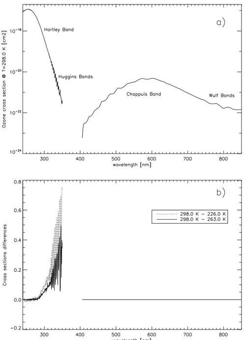
• Hartley band (200 nm< λ <310 nm); • Huggins bands (310 nm< λ <350 nm); • Chappuis band (480 nm< λ <610 nm); • Wulf bands (610 nm< λ <768 nm); • roto-vibrational band at ∼ 9.6 µ m.

In figure 1.8(a) the spectral absorption cross sections of ozone at T = 298.0 K are reported for UV and VIS bands. Figure 1.8(b) shows the spectral differences of the cross sections at different temperatures compared with the cross section at 298.0 K. As it is possible to notice there’s a remarkable temperature dependence of the absorption features of ozone in the UV bands, while no temperature dependence is reported in the VIS.

(26)

Figure 1.8: UV and VIS ozone absorption spectrum at T=298.0 K (a), and spectral differences of the cross sections at different temperatures (b). Elaborated from data

taken from [23]

(27)

1.3 Radiative transfer through the Earth’s atmosphere

1.3.1 Definition of radiometric parameters of interest

In this subsection the main parameters for radiative transport processes description will be defined. Please refer to [24] for more details.

The spectral radiant flux is defined as the rate of flow of electromagnetic energy across a surface dA whose normal versor is n0, at a given frequency:

F (r, n0, ν) =

d3E

dt · dA · dν (1.1) The spectral radiant flux units are [W/(m2Hz)]. The flux is dependent on the orientation of the elementary area: it is > 0 if energy is outgoing from the surface, viceversa if it is incoming. It is also possible to define two hemispheric fluxes, F↑(r, n0, ν) and

F↓(r, n0, ν), both > 0, as outgoing from or incoming to the surface, respectively. The

net spectral radiative flux is then:

F (r, n0, ν) = F↑(r, n0, ν) − F↓(r, n0, ν) (1.2)

The quantity F↓(r, n0, ν) is also called irradiance. It is also possible to define the

irradiance in the wavelengths domain:

F (r, n0, λ) = F (r, n0, ν) ·

c

λ2 (1.3)

To take into account the angular dependency of the energy flux the idea of radiance is introduced. Analogously to the definition of irradiance, we define a quantity d4_{E as the}

energy that flows in a solid angle dΩ in the direction Ω in the time interval dt at the frequency interval dν. The radiance is:

L(r, Ω, ν) = d

4_E

cos ϑ · dΩ · dt · dA · dν (1.4) The radiance units are [W/(m2Hz sr)]. Eq. (1.5) links the radiance and the irradiance.

F (ν) = Z Z 4π L(Ω, ν)dΩ = Z 2π 0 Z π 0 L(ϑ, ϕ, ν) · cos ϑ · dϑ · dϕ (1.5)

(28)

Finally we introduce the reflectance of a given surface as the ratio between reflected/s-cattered radiance and incident irradiance, in a given direction s0:

R(s0i, s0r, ν) = dLr(s0r, ν) dFi(s0i, ν) = dLr(s0r, ν) Li(s0i, ν) · cos ϑi· dΩi (1.6)

1.3.2 Radiative transfer equation

Starting from the definitions given in the previous section, we now want to analytically describe the problem of transport of radiation in Earth’s atmosphere. We want to derive the variations in the incident spectral radiance L(r, s0, ν) that crosses a cylindrical

volume of atmosphere with depth s in the direction s0.

The contributions to the variations in the radiance can be attributed to different sources:

• absorption of the medium; • scattering in different directions; • thermal emission of the medium; • scattering from different directions.

Let’s initially consider the different sources separately.

We first neglect the scattering contribution. The absorption and thermal emission con-tributions can be written as:

dL(s0, λ) = −kabs(λ) · ρ · L(s0, λ) · ds + kabs(λ) · ρ · B(λ, T ) · ds (1.7)

where kabs(λ) is the absorption coefficient, ρ is the medium density and B(λ, T ) is the

black body radiance at the temperature T.

We now consider the scattering contribution and neglect the absorption and thermal emission. The loss of energy due to scattering and the positive contribution from different directions is: dL(ϑ, ϕ, λ) = −ks(λ)·ρ·L(ϑ, ϕ, λ)·ds+ ks(λ) · ρ 4π Z 2π 0 Z π 0 P (ϑ, ϕ, ϑ0, ϕ0, λ)·L(ϑ0, ϕ0, λ)·sin ϑ0·dϑ0·dϕ0·ds (1.8)

(29)

where ks(λ) is the scattering coefficient and P (λ) is the phase function and identifies

how much radiation is scattered from an incoming direction (ϑ0, ϕ0) to a direction (ϑ, ϕ). So, with some simplifications, a general form of the radiative transport equation can be the following:

dL(λ)

dτ (λ) = −L(λ) + σ(λ) (1.9)

where σ(λ) is the source function and takes the general form:

σ(λ) = ω˜0 4π Z 2π 0 Z π 0 P (ϑ, ϕ, ϑ0, ϕ0, λ)·L(ϑ0, ϕ0, λ)·sin ϑ0·dϑ0·dϕ0+(1− ˜ω0)·B(λ, T ) (1.10)

The single scattering albedo ˜ω0 is the ratio of scattering and extinction components in

a radiation beam. We also introduced the optical depth τ , which is defined as follows:

τ (λ) = Z s0

s0

kext(λ)ds0 (1.11)

1.4 Height resolved atmospheric ozone measurements

Several methods to measure atmospheric ozone profiles and to retrieve height resolved information exist. Here we want to offer a state-of-the-art discussion on such methods; this is not intended to be a comprehensive survey but a useful summary to highlight the basic characteristics of the various ozone measurement techniques.

As for the measurement of other atmospheric parameters, atmospheric ozone measure-ment techniques can be divided into two main classes:

• in situ measurement techniques;

• remote sensing measurement techniques.

This latter class can be further divided into techniques with ground-based, satellite-borne and air-satellite-borne instrumentation.

(30)

1.4.1 In situ techniques

In situ measurements deal with instrumentation in contact with the object of interest. In the case of the ozone, the most typical in situ technique is related to ozonesondes (OS) [25].

The ozonesonde is a lightweight, balloon-borne instrument that is mated to a conven-tional meteorological radiosonde. As the balloon carrying the instrument package as-cends through the atmosphere, the OS telemeters to a ground receiving station informa-tion on ozone and standard meteorological quantities such as pressure, temperature and humidity. The balloon will ascend to altitudes of about 35 km or about 4 hPa before it bursts. The heart of the ozonesonde is an electrochemical concentration cell (ECC) that senses ozone as is reacts with a dilute solution of potassium iodide to produce a weak electrical current proportional to the ozone concentration of the sampled air. Air containing ozone is directed to one of the two platinum semi-elements, and the following reaction is triggered:

2 KI + O₃+ H₂O −−→ 2 KOH + I₂+ O₂

The produced iodine, on contact with the platinum cathode, reduces in the following way:

I₂+ 2 e− Pt−→ 2 I−

Iodine ions produce an electric current which is proportional to the ozone concentration. Ozonesondes provide accurate measurements with a very high vertical resolution. The main problem is the local nature of the measurements and high financial costs. The OSs are launched in a limited number of stations and typically at northern hemisphere mid-latitudes. In addition, differences in stations operations and changes in the employed technology limit the long term consistency of the method, especially when data from more than one station have to be compared. Usually OSs operates in networks as the World Ozone and Ultraviolet radiation Data Center (WOUDC) [26] or the Southern Hemisphere ADditional OZonesondes (SHADOZ) [20,27].

1.4.2 Ground-based remote sensing techniques

Height resolved and/or integrated quantities of ozone from ground-based remote sensing stations can be retrieved by means of passive or active instruments. Among passive

(31)

instruments we can identify the Dobson [25] and Brewer [28] spectrophotometers, and the Systeme d’Analyse par Observation Zenithale (SAOZ) spectrometer [29]. An active instrument in this field is the LiDAR [30].

The total column ozone can be measured from the ground using UV-absorption spec-troscopy. In particular, the two most common instruments are the spectrophotometers developed by G. Dobson and A. W. Brewer, respectively. The Dobson instrument is based on the differential absorption method in the UV band, where ozone exhibits strong absorption features. This method exploits the ratio of sunlight intensities at two wave-lengths characterized by strongly different ozone absorption cross sections. The Brewer spectrometer is similar in principle to the Dobson, but the determination of the ozone column amount is obtained from a combination of five wavelengths in the UV spectral range. An analogous instrument is the SAOZ, a UV-VIS spectrometer which measures the solar radiation scattered at the zenith in the spectral range 300-600 nm.

The application of the Umkehr principle to Dobson-Brewer instrumentation enables the retrieval of ozone concentrations at 10 different altitude layers, giving an estimation of the ozone vertical profile [31]. The height-resolved ozone distribution can also be obtained by millimeter-wave radiometers , which exploit a different spectral range. LiDAR instruments, which measure the attenuation and delay of a Rayleigh backscat-tered laser beam, have recently provided data of similar quality to the ozonesondes, spanning an altitude range of approximately 5-45 km [32]. Temporal sampling is po-tentially better than OS observations, but generally limited to cloud-free, night-time conditions.

1.4.3 Air-borne instruments

Air-borne techniques have some major advantages if compared to ground-based ones. These techniques allow the monitoring of extended areas; in addition, measurements can be directly done at the altitudes of interest and over regions that are difficult to cover by ground, as polar or tropical areas.

An interesting project that we want to mention here is the Air-Borne Lidar Experiment (ABLE), developed at “Sapienza” University of Rome [33]. This project aimed at the development of an air-borne LiDAR capable to take measurements at the typical upper troposphere/lower stratosphere altitudes.

(32)

1.4.4 Satellite-borne techniques

The orbits in which satellite-based ozone-profiling instruments can be successfully em-ployed are limited to Low Earth Orbits (LEOs), with altitudes typically between 600 and 900 km. They generally provide a global coverage of the Earth’s surface in few days. Besides absorbing in the UV, O3 has roto-vibrational spectral signature in the

mid-IR (see Sec. (1.2.4)) and a pure rotational signature extending into millimeter-wave spectral range. Remote sensing instruments for measuring atmospheric ozone from space therefore rely on spectroscopic or radiometric techniques, depending on the spectral interval used to perform the measurements.

Active techniques for atmospheric ozone observations, which exploit an actively induced detected signal, are currently restricted to the Differential Absorption LiDAR (DIAL) technique [32, 34]. In recent years a number of remote sounding satellites have been equipped with LiDAR instruments, see e.g. the PARASOL [35] or the CALIPSO mis-sions [36]; the technology, is mainly limited by the laser reliability and its power con-sumption.

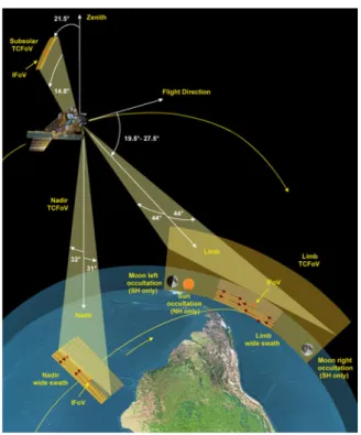
Passive techniques, on the other hand, have been successfully experimented during the last decades. Ozone remote sensing from space can be performed by observing the Earth’s natural radiation in different viewing geometries. The electromagnetic radia-tion reflected or emitted from the Earth’s atmosphere and/or from the surface can be measured by looking in the nadir or limb direction (see figure 2.5). Nadir observations generally provide a good horizontal resolution and sampling, but a limited vertical reso-lution which depends on the optical properties of the atmosphere and on the possibility to resolve in altitude the spectral signature. Limb sounders scan the atmosphere in the vertical, viewing tangentially to the reference spherical surface. Observed radiances are therefore predominantly sensitive to relatively narrow atmospheric layers close to each tangent point, allowing profiles with relatively high vertical resolution to be retrieved. Limitations of the technique are relatively poor horizontal resolution and sampling, and possibly lack of sensitivity to the lower atmosphere, due to obscuration by tropospheric humidity, clouds, aerosols or molecular scattering. The radiation can also be observed with a direct line of sight (LOS) between the source and the detector, which is done with solar, lunar or stellar occultation techniques. The high signal-to-noise ratio allows measurements to be made down to and below the tropopause, with high vertical reso-lutions. Observations are however limited by geometrical constraints, such that only a few tens of profiles can be measured per day.

(33)

1.4.4.1 Nadir viewing instruments

The total column of ozone has been continuously measured by the series of Total Ozone Mapping Spectrometer (TOMS) instruments since 1978 [37]. The first instrument ca-pable to provide an estimation of the ozone profile, namely the Backscatter UltraViolet (BUV) instrument, started its measurements in the early 1970s. It was followed by the Solar Backscatter UltraViolet (SBUV, 1978-1984) instrument [38] and by a series of SBUV-2 instruments [39, 40] starting in late 1984 on the operational satellite series of the National Oceanic and Atmospheric Administration (NOAA). This series is now continued as an U. S. national program with SBUV-2 instruments mounted on NOAA’s next generation National Polar Orbiting Environmental Satellite System (NPOESS). All these instruments perform the spectral measurement of the solar radiation backscattered by the atmosphere at 12 channels in the UV range, and can obtain height resolved ozone profiles by exploiting the large gradient in O3 optical depths across the Hartley-Huggins

bands. The Global Ozone Monitoring Experiment (GOME) [41], on board the second European Research Satellite (ERS-2) launched by the European Space Agency in 1995, enhanced this technique, providing the continuous spectrum between 240 and 790 nm, i.e. from the UV to the near-infrared (NIR) with relatively-high spectral resolution (∼ 0.2 nm). The wider spectral range of observation allows to obtain information on the ozone distribution coming also from the visible range (Chappuis band) by a Differential Optical Absorption Spectroscopy (DOAS) technique. The GOME instrument has been followed by the GOME-2 instrument carried on the Meteorological Operational (MetOp) satellite series as part of the European polar orbit satellite system [42]. The Scanning Imaging Absorption Spectrometer for Atmospheric Cartography (SCIAMACHY) on ESA’s En-vironmental Satellite (EnviSat) launched in 2002 can be considered as the successor of GOME, providing nadir observations of the solar backscattered radiation from 240 to 2380 nm [43]. In July 2004 the Ozone Monitoring Instrument (OMI) was successfully launched on the Earth Observing System Aura (EOS-Aura) satellite. OMI has similar capabilities for ozone profiling as the GOME and SCIAMACHY instruments, but with a much higher spatial resolution and a daily global coverage [44].

1.4.4.2 Limb viewing instruments

The Limb Radiance Inversion Radiometer (LRIR) and its successor the Limb Infrared Monitor of the Stratosphere (LIMS) instruments performed thermal emission measure-ments in the millimeter-wave and mid-IR spectral range since 1975 [45]. These in-struments can provide both day-time and night-time observations, exploiting the O3

emission lines for the ozone profile retrieval. The same principle has been used by the three instruments launched in 1991 as payload of the NASA Upper Atmosphere

(34)

Research Satellite (UARS), the Cryogenic Limb Array Etalon Spectrometer (CLAES) [46], the Improved Stratospheric And Mesospheric Sounder (ISAMS) [47] and the Mi-crowave Limb Sounder (MLS) [48]. Also the SubMillimeter Radiometer (SMR) on the Swedish experimental satellite Odin [49], launched in 2001, and EnviSat’s Michelson Interferometer for Passive Atmospheric Sounding (MIPAS) [50] instrument exploit such a technique to obtain ozone distribution. In the second half of the 1990s the Improved Limb Atmospheric Spectrometer instruments (ILAS-I and ILAS-II) were launched (on ADEOS-I and II, respectively), and performed limb spectral observations of the solar scattered radiation [51]. Unfortunately, both only produced data for a short period due to satellite problems. Other sensors have been conceived to perform limb-observations of the solar scattered radiation in the UV, VIS and NIR range, like the Optical Spectro-graph and Infrared Imager System (OSIRIS) [49], also carried on the Odin satellite, and SCIAMACHY on Envisat, see e.g. [52]. An improved version of the MLS, and the HIgh Resolution Dynamics Limb Sounder (HIRDSL), are part of the payload of NASA-Aura platform [53].

1.4.4.3 Occultation viewing instruments

Limb viewing occultation sensors observations started with the Stratospheric Aerosol and Gas Experiment (SAGE) in 1978 and are still operational [54]. Other instruments involve the second and third Polar Ozone and Aerosol Measurement (POAM-II and POAM-III on the French SPOT-3 and SPOT-4 satellites) [55], the Halogen Occultation Experiment (HALOE on UARS, still operational) [56], but also the previously-mentioned ILAS-I, ILAS-II and SCIAMACHY instruments. All these instruments view sun-rise and sun-set over the Earth horizon to measure the directly transmitted solar radiation along the line of sight. This technique has the limitation of providing only about 14 sun-rise and 14 sun-set measurement occasions per day, and in a specific latitude band, which changes with season or in time depending on the satellite orbit. The technique has been recently extended to include lunar (e.g. the SCIAMACHY) and stellar occultation (e.g. the Ultraviolet and Visible Imagers and Spectrographic Imagers (UVISI) [57] and the Global Ozone Monitoring by Occultation of Stars (GOMOS) [58]).

1.4.4.4 Ozone profiles retrieval from nadir UV/VIS satellite data

Ozone profiles can be retrieved from satellite measurements at different geometries and spectral bands. The use of nadir UV/VIS data has the advantage of providing a higher horizontal resolution than limb observations, still containing useful information in the UV/VIS sensible bands. Once the spectra are acquired the most notable problem is the

(35)

solution of the inverse problem leading from the measurement space to the ozone profile or state space (see Chapter3). Usually this task is performed by means of OE algorithms, i.e. algorithms to invert the physically-based forward radiative transfer model. To do this some a priori or climatological knowledge is necessary, i.e. the average/climatological ozone profile and covariance matrix. OE algorithms were used for the estimation of ozone profiles from the SBUV, see e.g. [59] and the GOME, see e.g. [60]. An alternative physically-based technique is the Philips-Tikhonov regularization approach, which has been applied to GOME nadir UV/VIS data [61]. An alternative methodology is related to statistical models as the NNs. NNs algorithms were applied to GOME data, see e.g. [62, 63]. In the context of GOME data inversion, these different algorithms and their performances were compared, and results are shown in [64]. Known issues in OE methods regard the sensitivity to systematic/calibration errors and any problem regarding the incomplete formulation of the used forward model, as interactions with clouds and/or aerosols; these problems may be circumvented by the use of NNs.

1.4.4.5 Tropospheric ozone retrieval from nadir UV/VIS satellite data

The retrieval of tropospheric ozone information from space is a particularly difficult task. The problems discussed for the ozone profiles retrieval magnify at lower levels, where a scarce sensitivity is also present. Moreover, a high horizontal resolution is even more important than higher altitude levels, owing to the environmental and air quality implications and short-term space variations involved. A classical approach to this issue is the computation of the TOCs by means of the TOR technique. To separate stratospheric and tropospheric contributions, usually a cloud slicing technique is adopted. Once the tropopause height is determined, the TOC is estimated starting from two measurements, e.g. one nadir instrument operating in the UV measuring the total ozone column content, and one instrument measuring the stratospheric ozone concentrations, e.g. a MW limb sounder as MLS. Examples of this approach are in [65–70]. Another method to retrieve the TOC is the integration of ozone concentrations from OE algorithms over tropospheric altitudes.

1.5 Thesis outline

This thesis is structured in the following way:

• Chapter 2 briefly discuss the SCIAMACHY and OMI missions; data from these sensors have been considered in this thesis work;

(36)

• Chapter 3 offers a description of the existing inversion algorithms; first gives an introduction of OE methods and then an overview of the NNs. The two classes of algorithms are put in the same context of the inversion of Earth’s spectra to retrieve height resolved atmospheric parameters;

• Chapter 4 presents a new approach to the direct retrieval of tropospheric ozone information from nadir UV/VIS satellite data, with a particular emphasis to the SCIAMACHY nadir states. NNs algorithms are used. The developed algorithm is discussed, as well as design issues and input vector dimensionality reduction by means of an RTM-EP combined algorithm;

• Chapter5presents a NNs approach to the retrieval of vertical ozone concentration profile from SCIAMACHY data. As for Chapter 4, design issues are critically discussed. Results are compared to matching retrievals based on the GOME in-strument;

• Chapter 6 presents a NNs approach to the retrieval of stratospheric ozone con-centration profiles from OMI data. As for Chapter 4, design issues are critically discussed. This part of the work has been performed during a 6 months visit to NASA-GSFC, Greenbel, MD, USA, under the direction of P. K. Bhartia.

• Chapter3gives conclusions and future outlook.

• AppendicesAandBshow further work performed during the PhD period, includ-ing the design of a validation activity for NNs algorithms in a GRID environment, and the development of NNs algorithms for the retrieval of additional atmospheric parameters, like temperature profiles and nitrogen dioxide concentrations.

(37)

Chapter 2

The SCIAMACHY and the OMI

missions

This Chapter introduces two satellite sensors whose data have been used in this work: the EnviSat-SCIAMACHY and the Aura-OMI. A description of these sensors is given in Sec.s (2.1) and (2.2), and some issues regarding operations, calibration and monitoring of their performances are discussed therein.

2.1 The SCanning Imaging Absorption spectroMeter for

Atmospheric CHartographY (SCIAMACHY)

2.1.1 The EnviSat Platform

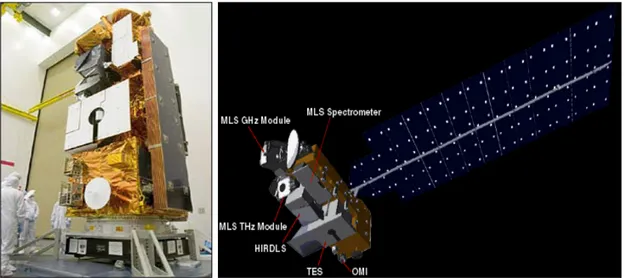
The EnviSat Platform is part of ESA’s Earth observation mission [71]. Envisat is an advanced polar-orbiting Earth observation satellite that provides measurements of the atmosphere, ocean, land, and ice by means of its payload composed of 10 instruments. It is intended to give continuity to the ESA ERS missions. With an overall length of more than 25 m, it is the largest satellite ever built by ESA [71]. Fig. (2.1) shows the platform during integration at ESA-ESTEC, with reference to the various sensors in its payload.

Envisat flies in a sun-synchronous polar orbit of about 800 km altitude. The repeat cycle of the reference orbit is 35 days, and for most sensors, being wide swaths, it provides a complete coverage of the globe within one to three days [72]. Some general and orbital parameters are reported in Tab. (2.1).

(38)

Chapter 2. The SCIAMACHY and the OMI missions 29

Figure 2.1: EnviSat during integration in ESA-ESTEC, the Nederlands. Courtesy of Dutch Space. General Parameters Dimensions 26 m × 10 m × 5 m Total Mass 8140 kg Payload Mass 2050 kg Launcher Arianne-5 Launch Date March, 1st_{, 2002}

Orbital parameters

Inclination 98.55 ± 3 Mean Altitude 799.8 km Orbital Period 100.6 min

Orbital Type Polar, sun-synchronous Orbits per day 14 11/35

Repeat Cycle 35 days (501 orbits)

Table 2.1: EnviSat parameters. Adapted from [72].

2.1.2 The instrument

The SCIAMACHY instrument, onboard the ESA-Envisat spacecraft, is a nadir/limb/lu-nar and solar occultation viewing spectrometer that can operate in the UV/VIS/NIR range (214 to 2386 nm), with a spectral resolution of 0.24-1.48 nm (0.24-0.48 nm in our spectral region of interest) and a nadir spatial resolution of typically 30 km along track × 60 km across track [72–74]. The SCIAMACHY is a passive imaging spectrometer. It is made by the following three elements:

• optical assembly (OA), composed by a mirror system, a telescope and a spectrom-eter;

(39)

Figure 2.2: Sciamachy level 1 OA. Courtesy of DLR-IMF.

• thermal subsystem; • electronic subsystems.

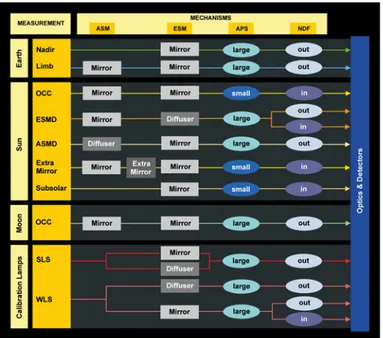
The OA is the part of the instrument that collects light and produces the spectral information. For maintaining the specified thermal conditions, the OA includes a radi-ator and the so-called Thermal Bus Unit (TBU). The OA is organized into two levels; Fig.s (2.2) and (2.3) depict these two parts of the OA. Entrance optics, pre-disperser prism, calibration unit and channels 1 and 2 are contained in level 1 OA facing in the flight direction. Channels 3-8 are located in level 2 OA. By combining the optical components various optical paths or trains from external and internal light sources to detectors can be established, so identifying the various observation modes of the instru-ment (cfr Fig. (2.4)). During nominal measurements light enters the instrument via the Azimuth (ASM) or Elevation Scan Mechanisms (ESM). Whilst the ASM captures radiation coming from regions ahead of the spacecraft, the ESM either views the ASM or the region directly underneath the spacecraft. In the first case (limb observation), the light collected from the ASM is reflected into the spectrometer, in the second case (nadir observation) the ASM is not involved in the optical path. The scanning interval of the two scanning mechanisms is limited by baffles; the effective or Total Clear Field of View (TCFoV) is then the one discussed in Sec. (2.1.3) for the different observation modes. The scanner control tasks are programmed in on-board software with support-ing information besupport-ing generated by the Sun Follower (SF) in the case of solar and lunar observations. The solar irradiance has to be measured via a diffuser. Two aluminium

(40)

Figure 2.3: Sciamachy level 2 OA. Courtesy of DLR-IMF.

Figure 2.4: Sciamachy observation modes and related optical paths or trains. Cour-tesy of DLR-IMF.

(41)

Channel Spectral Range (nm) Resolution (nm) Stability (nm)

1 214-334 0.24 0.003 2 300-412 0.26 0.003 3 383-628 0.44 0.004 4 595-812 0.48 0.005 5 773-1063 0.54 0.005 6 971-1773 1.48 0.015 7 1934-2044 0.22 0.003 8 2259-2386 0.26 0.003

Table 2.2: SCIAMACHY science channels. Adapted from [72]

diffusers are mounted on the SCIAMACHY: one on the backside of the ESM mirror, one on the backside of the ASM mirror.

The ESM reflects light towards the telescope mirror, which has a diameter of 32 mm. From the telescope mirror the light path continues to the spectrometer entrance slit. The overall spectrometer design is based on a two stage dispersion concept: first, the incoming light is pre-dispersed and projected onto a spectral image. Subsequently, this spectral image is dissected into eight spectral intervals that are diverted into eight spec-tral channels for further dispersion. The selected approach has the advantage of reducing stray light in the channels with average low light intensity ( e.g., UV and NIR-SWIR). The pre-disperser prism, located behind the entrance slit, is used for two purposes: it weakly disperses the light and directs fully polarized light for further processing to the Polarization Measurement Device (PMD). Small pick-off prisms and subsequent dichroic mirrors direct the intermediate spectrum to the 8 science channels where the light is further dispersed by individual gratings. In the light path routed to channels 3-6 the Neutral Density Filter Mechanism (NDFM) can move a filter into the beam. With a filter transmission of 25% it can be used to reduce light levels during solar measurements. The full resolution spectral information is generated in 8 science channels (see Tab. (2.2)). These employ two types of detectors. For the UV-VIS-NIR range covered by channels 1-5, standard Silicon photodiodes (RL 1024 SR, EG&G RETICON, California) with 1024 pixels are used which are sequentially read out. Additionally, UV channels 1 and 2 are electronically divided into two virtual bands 1a/1b and 2a/2b, which can be configured separately. The SWIR channels 6-8 employ Indium Gallium Arsenide detectors (InGaAs by EPITAXX, New Jersey) specifically developed and qualified for SCIAMACHY.

For channels 1-5, the detector pixels are read out sequentially with a time delay between the first and the last pixel of about 28.75 msec. Therefore pixels that are read out at a different time see a somewhat different ground scene because during the sequential readout the platform and the scan mirrors continue to move. The size of the wavelength

(42)

dependent spectral bias depends on the variability of the ground scene. Nominally, the minimum Pixel Exposure Time (PET) amounts to 31.25 ms. Trace gas features are distributed non-uniformly over the spectrum. The limited total data rate would therefore prohibit the detailed sampling of those ranges of interest if the full spectrum had to be downlinked as one block. SCIAMACHY avoids this situation by using spectral clusters and co-adding. The 1024 pixels per channel can be sub-divided into a number of clusters identifying regions where trace gas retrieval will take place. Each cluster can be sampled by on-board data processing applying co-adding factors fcoadd to the readout

of the pixels of this cluster. This results in an Integration Time (IT ):

IT = tPET· fcoadd (2.1)

which defines how many subsequent readouts of each pixel of a cluster are added to generate one measurement data readout. By appropriately setting the integration time, high or low temporal resolution, equivalent to high or low spatial resolution, can be selected. Thus, depending on the executed measurement states, variable ground pixel sizes as a function of spectral region, i.e. trace gas features, are achieved. Overall the detector performance is characterized by low noise and high instrument throughput. This allows measuring the incoming light with the required very high signal-to-noise ratio [74].

The requirements to maintain high spectral stability and relative radiometric accuracy over the mission’s lifetime is verified via an on-board calibration unit. It consists of two calibration lamps, one for white light and one for spectral lines. The White Light Source (WLS) is a 5 Watt UV-optimized Tungsten-Halogen lamp with an equivalent blackbody temperature of about 3000 K. Its signal is used to verify the pixel-to-pixel signal stability. The Spectral Line Source (SLS) is a Neon filled hollow Pt/Cr cathode lamp. Its operation allows the determination of the pixel-to-wavelength relation. The calibration unit is located close to the ESM. By rotating the ESM mirror into specific positions it is possible to reflect light from the WLS respectively the SLS towards the telescope mirror and thus onto the entrance slit.

The measurement sensitivity of the spectrometer depends on the polarization state of the incoming light. Therefore SCIAMACHY is equipped with a PMD. Six of its channels (PMD A-F) measure light polarized perpendicular to the SCIAMACHY optical plane, generated by a Brewster angle reflection at the second face of the pre-dispersing prism. This polarized beam is split into six different spectral bands. The spectral bands are quite broad and overlap with spectral regions of channels 2, 3, 4, 5, 6, and 8.

The Optical Bench Module (OBM) needs to be operated in orbit at a constant tempera-ture to preserve validity and accuracy of the on-ground calibration and characterization.