Scattering networks: efficient 2D implementation and application to melanoma classification

Alma Mater Studiorum · Universit`

a di Bologna

Scuola di Scienze

Dipartimento di Fisica e Astronomia Corso di Laurea Magistrale in Fisica

Scattering Networks: Efficient 2D

Implementation And Application To

Melanoma Classification

Relatore:

Prof. Renato Campanini

Correlatore:

Dott. Matteo Roffilli

Presentata da:

Eugenio Nurrito

Abstract

Machine learning is an approach to solving complex tasks. Its adoption is growing steadily and the several research works active on the field are publishing new interesting results regularly.

In this work, the scattering network representation is used to transform raw images in a set of features convenient to be used in an image classification task, a fundamen-tal machine learning application. This representation is invariant to translations and stable to small deformations. Moreover, it does not need any sort of training, since its parameters are fixed and only some hyper-parameters must be defined.

A novel, efficient code implementation is proposed in this thesis. It leverages on the power of GPUs parallel architecture in order to achieve performance up to 20× faster than earlier codes, enabling near real-time applications. The source code of the implementation is also released open-source.

The scattering network is then applied on a complex dataset of textures to test the behaviour in a general classification task. Given the conceptual complexity of the database, this unspecialized model scores a mere 32.9 % of accuracy.

Finally, the scattering network is applied to a classification task of the medical field. A dataset of images of skin lesions is used in order to train a model able to classify malignant melanoma against benign lesions. Malignant melanoma is one of the most dangerous skin tumor, but if discovered in early stage there are generous probabilities to recover. The trained model has been tested and an interesting accuracy of 70.5 % (sensitivity 72.2 %, specificity 70.0 %) has been reached. While not being values high enough to permit the use of the model in a real application, this result demonstrates the great capabilities of the scattering network representation.

Sommario

Il machine learning `e un approccio alla risoluzione di problemi complessi. Il suo

utilizzo `e in costante crescita e i diversi lavori di ricerca attivi nel settore pubblicano

regolarmente nuovi, interessanti risultati.

In questo lavoro si adopera la rappresentazione scattering network per trasformare immagini grezze in un insieme di features utilizzabili per la classificazione di immagini,

un’applicazione fondamentale del machine learning. Questa rappresentazione `e

invarian-te per traslazioni ed `e stabile alle piccole deformazioni. Non necessita inoltre di alcun

tipo di addestramento, poich´e i suoi parametri sono fissi e solo alcuni iper-parametri

devono essere definiti.

In questa tesi `e proposta una nuova ed efficiente implementazione del codice. Essa

sfrutta la potenza dell’architettura parallela delle GPU per raggiungere performance fino

a 20 volte pi`u veloci dei codici precedenti, consentendo la realizzazione di applicazioni

quasi in tempo reale. Il codice sorgente dell’implementazione `e inoltre rilasciato

open-source.

La scattering network `e poi applicata ad un dataset complesso di texture per

testar-ne il comportamento in un problema getestar-nerico di classificaziotestar-ne. Data la complessit`a

concettuale del database, questo modello non specializzato raggiunge un mero 32.9 % di accuratezza.

Infine, la scattering network `e applicata ad un problema di classificazione in

ambi-to medico. Un dataset di immagini di lesioni della pelle `e utilizzato per addestrare un

modello che possa classificare melanomi maligni contro lesioni benigne. Il melanoma

ma-ligno `e uno dei pi`u pericolosi tumori della pelle, ma, se scoperto in uno stadio precoce,

le probabilit`a di cura sono elevate. Il modello addestrato `e stato testato ed `e stata

rag-giunta un’interessante accuratezza del 70.5 % (sensibilit`a 72.2 %, specificit`a 70.0 %). Pur

non essendo valori abbastanza elevati da permettere l’utilizzo del modello in

un’applica-zione reale, i risultati dimostrano le grandi possibilit`a della rappresentazione scattering

Contents

1 Introduction 1

2 Machine Learning and Scattering Convolutional Networks 3

2.1 Toward Scattering Convolutional Networks . . . 4

2.2 Scattering Convolutional Network . . . 6

2.3 The Algorithm . . . 8

2.3.1 Downsample . . . 9

2.3.2 Pre Computing Filters . . . 10

2.3.3 Reduced Scattering Transform . . . 10

2.3.4 Convolution Filtering and Convolution Theorem . . . 10

2.3.5 Padding . . . 11

3 GPU Implementation of Scattering Convolutional Networks 13 3.1 GPU computing with CUDA . . . 14

3.2 Software Tools . . . 15 3.2.1 Numpy . . . 16 3.2.2 PyCuda . . . 16 3.2.3 Scikit-Cuda . . . 16 3.2.4 OpenCV . . . 17 3.3 Development . . . 17 3.3.1 First implementation . . . 17 3.3.2 Second Revision . . . 18 3.3.3 Latest release . . . 19

3.5 Compatibility Tests . . . 22

3.6 Performance . . . 25

4 Training and Test Methodology of a Machine Learning Problem 35 4.1 Train/test sets and cross-validation . . . 35

4.2 Pre-processing . . . 36

4.3 Data Augmentation . . . 37

4.4 Feature Extraction . . . 37

4.5 Feature scaling . . . 38

4.6 Classifier training . . . 38

4.6.1 Support Vector Machine . . . 39

4.7 Implementation and practical details . . . 40

5 Textures Classification 43 5.1 Database . . . 43 5.2 Classification Results . . . 44 6 Melanoma Classification 47 6.1 Introduction . . . 47 6.2 Database . . . 49

6.3 Model training and results . . . 51

7 Conclusions 57

CHAPTER

1

Introduction

In the last decade, the world faced with the concept of “big data”. This term refers to the great mole of organized, accessible and growing information coming from assorted groups of measures. The introduction of this concept was made possible by the incessant

evolution of electronics and information technology. Electronics contributed making

available cheap and fast sensors for every needing: imaging, chemical analysis, physical measures are only some examples. Information technology, in its turn, provided the software and hardware platforms to analyze obtained information. New devices, with different architectures (CPU, GPU, DSP, FPGA, ...) and with increasing power in terms of FLOPS, are available every day.

Many approaches were used during the years to analyze this data. The ultimate goal is to use data to understand a trend and, consequently, make predictions and take decisions. Statistics has always been used for this purpose. But even if simple statistics approaches were usually enough to deal with a limited amount of controlled data in the past, the challenge of analyzing “big data” is to extrapolate information in situations that were not represented by available data, thus to be able to generalize.

“Machine learning” is a term that can be heard around every day. This approach consists in training a model to make predictions basing on parameters learned from available data. Classical approaches, intead, have the difference of having little or none information of data included in the structure of the model. Therefore, machine learning algorithms are able to generalize, and well.

Many applications are now based on machine learning and the medical field is no exception. Histological and cytological images can be analyzed by an algorithm that detects and classifies each single cell. This helps physicians to classify microscopy samples

faster. CAD systems (Computer Aided Detection/Diagnosis system) based on machine learning are present in many areas, for example to automatically recognize masses and microcalcifications in mammograms [1].

In this thesis, the “scattering convolutional network” concept is used. This method, proposed by S.Mallat and J.Bruna in [2, 3], allows to create a representation of a signal (in our case an image) that is invariant to translations and stable to deformations. Backed by the important results obtained by the wavelets proposed by the same Mallat, the scattering convolutional network offers an interesting way to extract features of a signal, that should allow a machine learning algorithm to learn a generalization of the problem. Chapter 2 starts with an introduction to what a “machine learning algorithm” is and then explains the scattering convolutional network algorithm.

One of the contributions of the thesis work is the realization of the scattering network algorithm in code capable of running on GPUs, thus improving time performance over the original serial code. Chapter 3 shows how an efficient implementation has been studied over several revisions, with analysis of compatibility tests and the final performance improvement. Moreover, the written source code has been released open source with the hope to help other researchers in future studies or applications with the scattering network algorithm.

The interest then moved to classification. In this task, the theory of scattering net-works suggests that they are able to create a discriminable representation with important stabilities. Chapter 4 presents the general methodology used to train and test a classifier, with punctual details on the actual procedure used in the following two applications.

Since studies on scattering networks appeared to work well in recognizing patterns and textures, the algorithm has been firstly tested in Chapter 5 to extract features from the recent “Describable Textures Dataset” [4]. This application was mainly a first attempt to understand the possibilities of the algorithm toward a more practical application.

A medical field where machine learning is still at an early stage is dermatology. A particular task where it is gradually acquiring interest is melanoma classification. The investment on this problem arises from the possibility to cure by biopsy a malignant melanoma if it is detected in the early phase of development. Therefore, if an automatic system could perform a preliminary diagnosis, possible malignant melanoma could be discovered in time to be treated. Chapter 6 sets out an attempt to classify a skin lesion (nevi) to be either a benign lesion or a malignant melanoma. This task is dealt with a model based on a scattering network representation and a SVM classifier. A recent valuable database from the ISDIS (International Society for Digital Imaging of Skin) [5] is used. The main intention of this application was not to try to reach a state-of-the-art comparable results, but to test if the general purpose scattering network algorithm could give interesting results in an application of practical utility and of common interest.

The work of thesis was mainly developed in Bioretics’ offices[6], a start-up company whose primary interest is solving imaging and computer vision problems.

CHAPTER

2

Machine Learning and Scattering Convolutional

Networks

Machine learning is the field of computer science that tries to create algorithms that are able to learn from a set of data. Mitchell [7] wrote a definition of a learning algorithm: Definition 2.1. A computer program is said to learn from experience E with respect to some class of tasks T and performance measure P, if its performance at tasks T, as measured by P, improves with experience E.

We can recognize in the experience E the big data available nowadays, that can spread over a great range of fields. The concept of performance measure P is also very broad, as it ranges from objective metrics to individual judgments. Nevertheless, measure P is usually specific to the task T. Tasks, instead, can be usually grouped by their type. Most common kinds of task are classification, regression, clustering, density estimation and feature reduction.

In this work, we will deal mainly with classification. A classification task consists of assigning an input sample to a category (also called class, whose name is defined label).

Thus, a machine learning algorithm needs to learn a function f : Rn_{→ {1, . . . , k}, which}

map the n dimensional input to one of the k categories. A common, but complex, example of classification is image recognition, in which the algorithm is required to output a label for the input image.

At the baseline, a classification task consists of a measure of similarity. Simple Eu-clidean distance is generally unable to discriminate and give good measures of similarities on real world data where intra-class variability is relevant.

Continuing with the example of image classification, there is a great variability in images belonging to the same class, due to rigid and non-rigid transformations. In fact, a simple operation like a translation can create a great variation of the value of each pixel of the image. This intra-class variability is an obstacle to classification and must be eliminated in order to have a more informative measure of similarity. The general approach to this problem is based on Kernel Methods [8], who consist of projecting input data x in a new representation Φ(x). This could allows to build a representation that is invariant to some transformations. History of physics teaches that most modern theory are founded on the presence of symmetries and thus invariants in a system. Having a representation of this could easily lead to good subsequent results.

In the image field, rigid transformations such as translations, scaling and rotations are generally uninformative for classification. Therefore a good representation should be invariant to this kind of deformations. In fact, they are usually caused only by the relative pose of the object with respect to the camera, an information that in most application is in inconspicuous. On the other side, non-rigid deformations may induce both intra-class and inter-class variability. For example, a non-rigid deformation could transform a “1” into a “7”, and thus changing the outcome of a digits recognition system. A good representation Φ(x) for classification should therefore not be deformation invariant, but stable to small deformations [3]. This will allow to discriminate between different classes with a kernel classifier. In fact, the kernel will permit to handle the small deformations.

The stability to deformations is expressed as a Lipschitz continuity condition. Given

a deformation Lτx(u) = x(u − τ (u)) where x is an image, u the position inside the image

and τ (u) the function that gives the deformation, we can express the gradient of the transformation ∇τ (u), whose norm |∇τ (u)| measures the amplitude of the deformation. Therefore, a representation Φ(x) is stable to deformations if it is Lipschitz continuous relative to the deformation metric:

kΦ(Lτx) − Φ(x)k ≤ Ckxk sup

u

|∇τ (u)|

where kxk =R |x|2_du.

Getting rid of variance due to small deformations, a good representation must pre-serve (and enhance) the discriminability that lays in information given by high-order moments.

2.1

_{Toward Scattering Convolutional Networks}

The problem is to find a “good” representation Φ(x) for the data, as expressed before. It should be stable to additive noise and small deformations and it should carry information of high-order moments for discriminability. In the treatment we will also impose the

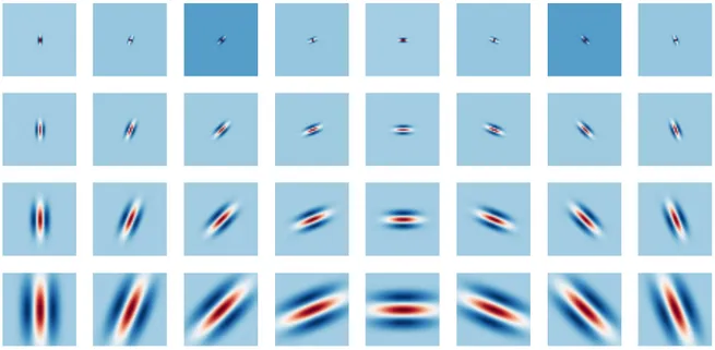
stronger requirement to the representation to be (locally) translation invariant. Features for this representation could be extracted by filtering with wavelet filters the input signal. Wavelets are wave-like functions localized in both space and frequency [9] and thus they are stable to deformations. Given a single band-pass wavelet ψ(u), it is possible to build a bank of multiscale directional wavelets:

ψ2j_r = 22jψ(2jr−1u)

where j ∈ Z and r ∈ G, with G a finite rotation group in R2_{. Let’s denote λ = 2}j_{r for a}

simpler notation. An example of a filters bank of this kind can be seen in Figure 2.1.

Figure 2.1: A filter bank of complex Gabor wavelets with 4 scales and 8 orientations. Only the real part is displayed.

Given a family of wavelets {ψλ(u)}λ, the operation of convolving a signal x with each

wavelet ψλ is called wavelet transform and is defined {x ? ψλ}λ where each element of

the set is called wavelet coefficient.

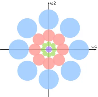
If the wavelet set covers the entire frequency plane (as illustrated in Figure 2.2), the wavelet transform is stable to deformations and invertible.

In particular, the wavelet transform is linear, so it is translation covariant, not in-variant. [3] shows that a non-linearity is needed to build a translation invariant repre-sentation. This is chosen to be the modulus operation, a point-wise non-linearity that preserves deformation stability and conserves the energy. Conceptually, the modulus smooths the complex wavelet coefficients, pushing high frequencies to lower ones.

Figure 2.2: Representation of a uniform and complete covering of the frequency plane by a set of scaled and rotated wavelets.

A translation invariant representation is obtained by applying the only linear operator stable to translation: the average. For the classification task, it’s often better to have

a local stability. This means having a local averaging, i.e. a blurring operator φ2J on a

spatial window of size 2J_{. The result is a translation invariant wavelet coefficient:}

SJ[λ]x = |x ? ψλ| ? φ2J

Unluckily, this operation will kill the high-order moments that lead to discriminability. Lost information can be recovered by applying this same procedure to U [λ]x, obtaining:

SJ[λ1, λ2]x = ||x ? ψλ1| ? ψλ2| ? φ2J

where ψλ1 and ψλ2 belong to the same wavelets family. This procedure can be applied

iteratively to extract wavelet coefficients of higher order moments.

Any sequence p = (λ1, λ2, ..., λm) is called a “path” of length m, hence:

SJ[p]x = ||||x ? ψλ1| ? ψλ2|...| ? ψλm| ? φ2J

This approach naturally creates a convolutional network structure.

2.2

_{Scattering Convolutional Network}

The scattering convolutional network is the representation composed of all coefficients

Given a signal x, all coefficients SJ[p]x are obtained from a layered structure, where

the scattering propagator UJx = {x ? φ2J, |x ? ψ_λ|}_λ is iteratively applied to obtain the

path p. An illustration of a scattering convolutional network can be seen in Figure 2.3.

Figure 2.3: A graph representation of a scattering neural network from [2]. Scattering

propagator UJ is applied to f to compute U [λ1]f and outputs S[0]f . UJ is then applied

to every U [λ1] to obtain the second layer of the scattering and relative outputs. This

iteration is repeated up the required depth.

The signal representation offered by scattering networks has several important prop-erties.

First of all, no parameter needs to be learned to perform the transformation. Only some hyper-parameters could be selected with some tests. This is opposed to common convolutional neural networks, where the filters need to be learned from the data with the back-propagation algorithm.

Secondly, it is invariant to translations up to 2J _{because of the final averaging}

win-dows. This property is essential in image classification where a small translation rarely influences the category.

Then, as previously stated, with a suitable set of wavelets the representation is stable to deformations. This guarantees that small deformations that shouldn’t affect classifica-tion result can be completely managed by a kernel classifier. Some further works on the scattering network included stability to other particular transformations. For example, in [10] a further stability to rotations is inserted in the structure of the representation by combining signals scattered from different rotations of the filters. Other stabilities could be included if the mathematical formulation could be given. Beside that, this work will only deal with the classic formulation of the scattering network.

Finally, it has been proved that, with a proper set of wavelet, the scattering operator

UJx is contractive, in the sense that kUJx − UJyk ≤ kx − yk and it also preserves signal

zero when mmax increases. This is important in numerical applications because it allows

to keep the network depth low with a negligible loss of energy.

A common set of wavelets used for the scattering network representation is based on scaled and rotated Gabor Wavelets (an example is shown in Figure 2.1). These wavelets are basically a Gaussian function modulated by a complex exponential. Other kinds of wavelets have been used, for instance Haar wavelets [11].

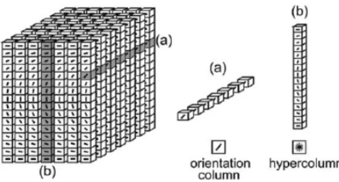
Considering Gabor wavelets, an analogy with the visual system of mammals can be proposed. In fact, Hubel and Wiesel [12] and subsequent studies suggested that primary visual cortex V1 is formed by neurons whose response has the same kind of shape of Gabor wavelets. These neurons are organized in hypercolumns (Figure 2.4), and the position of each neuron in the column defines the orientation, the scale and the location of the patterns of light that it recognizes. Scattering convolutional networks follows a similar approach, decomposing the input signal by the response of scaled and rotated Gabor wavelets, although the translation (location) is chosen to be an invariant by construction.

Figure 2.4: An illustration of hypercolumns in the primary visual cortex. Each box is a neuron that responds to a particular orientation and scale of light patterns. From [13].

2.3

_{The Algorithm}

Illustration of Figure 2.3 suggests to calculate the scattering network representation iterating layer by layer, i.e. increasing the length of paths p.

Let’s call Λm_J the set of all paths p = (λ1, ...λm) of length m. We define also the set

of all U and SJ computed for paths of length m as U [ΛmJ] = {U [p]x}p∈Λm

J and SJ[Λ

m J] =

{SJ[p]x}p∈Λm

J. Finally let’s define the set ΛJ = {λ = 2

j_{r : r ∈ G}+_{, j ∈ Z, j ≥ −J}}

The scattering network representation of a signal x can be computed with the base Algorithm 1.

The algorithm is iterative and uses previously calculated U [Λm−1_J ] to compute new

data at layer m. In this way, each path p is composed step by step to avoid the evaluation of the same expressions multiple times.

Algorithm 1 Scattering Network Algorithm 1: U [Λ0

J] ← x

2: for m = 1 to M do . for each layer

3: Compute every U [Λm_J] = {|U [Λm−1_J ] ? ψλ|}λ∈ΛJ . band-pass filtering and modulo

4: Output every SJ[ΛmJ]x = U [Λ

m−1

J ]x ? φ2J . output low-pass filtering

5: end for

This version of the algorithm is also expressed in a very synthetic style. A real implementation of the algorithm should make sure to iterate over every path p and every

filter ψλ. If the value of parameters M , J and L grows, the number of operations to

perform increase exponentially with M. It can be seen that the total number of elements U [p] and SJ[p] is 1 + (J · L)M, giving a total of 2 · [1 + (J · L)M] convolution operations.

Starting from this pseudo-code, a real implementation of the scattering network al-gorithm can use several expedients to achieve good performance. Some of theme are exposed in subsequent paragraphs.

2.3.1 Downsample

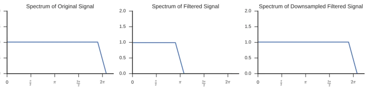
When a signal is passed through a bandpass or a lowpass filter, it may be possible to uniformly downsample it without losing information, according to the Shannon-Nyquist’s rule. For example, a half band lowpass filter would allow to discard every other sample, because after the filtering the signal has the highest frequency half of the original one (as illustrated in Figure 2.5). This allows to remove redundant information with the benefit of having a more compact representation.

0 π 2 π 32π 2π 0.0 0.5 1.0 1.5 2.0 Spectrum of Original Signal 0 π 2 π 32π 2π 0.0 0.5 1.0 1.5 2.0 Spectrum of Filtered Signal 0 π 2 π 32π 2π 0.0 0.5 1.0 1.5 2.0 Spectrum of Downsampled Filtered Signal

Figure 2.5: An illustration of the FFT spectrum after a low-pass filtering (center) and a downsample (right).

In the scattering network, both ψ₂J and φ_λ are filters that lower the frequency band

of the signal (except when j of λ is 0). The averaging with ψ₂J allows to downsample

SJ[p]x at intervals 2J. Instead, band-pass filters φλ reduce frequency band with respect

Using this technique, if the signal x is an image of N pixels, the coefficient SJ[p]x

will have only 2−2JN elements.

The application of this method to the algorithm previously described will allow to compute simpler operations. Indeed, the signals size will decrease through paths. How-ever, some care must be used to decide the right sample interval at each step of each

path. Final signals must not be subsampled at intervals more than 2J _{in total.}

2.3.2 Pre Computing Filters

The wavelet filters bank {ψλ(u)}λ∈ΛJ is fixed and reused several times during the

exe-cution of a scattering network. Therefore, a major optimization is to pre-calculate the filters from the required hyper-parameters M , J and L of the scattering network. As this operation could take a remarkable amount of time, wavelet filters banks could also be cache stored on disk to improve performance in multiple runs.

Filters can be generated in the spatial space or in the frequency space. The first method does not need to know the original image size to create filters. Instead, in order to create filters directly in the Fourier space, a fundamental requirement is the previous knowledge of the image size. This way, the filter generator can create the appropriate filters for each possible subsample of the original signal throughout the scattering paths of the network.

2.3.3 Reduced Scattering Transform

In [3], authors showed that scattering energy is concentrated along frequency-decreasing paths p. This means that all paths where index j decreases can be omitted from com-putation with negligible loss of energy and thus quality of the representation for classifi-cation. Instead, this approach allows to implement a noticeably faster algorithm, where lots of paths are discarded (in particular those with low j that contains larger signals in the downsample approximation, which are the ones that would require more time to be computed). The resulting representation is called “Reduced Scattering Transform” and derives directly from the original algorithm by adding checks on which λ to use to compute new U [Λm_J].

2.3.4 Convolution Filtering and Convolution Theorem

The convolution operation is clearly the most present and time consuming operation in the proposed algorithm.

Let’s recall from [14] that given two continuous functions f (t) and h(t) of the con-tinuous variable t, the convolution is defined as:

f (t) ? h(t) =

Z ∞

−∞

Applying the Fourier transform to f (t) ? h(t) gives the Fourier pair: f (t) ? h(t) ⇔ F (ω)H(ω)

and a similar procedure would also give:

f (t)h(t) ⇔ F (ω) ? H(ω)

These two pairs are called the Convolution Theorem. It states that a convolution in one of the spaces is equivalent to a point-wise multiplication in the other space.

The convolution theorem applies also to discrete signals, but periodicity problems may arise. Discrete functions have a periodic Fourier spectrum, as explained by the “sampling theorem”, so the convolution with the convolution theorem would give a periodic convolution, also called “circular convolution”. This creates a “wrap-around error” at boundaries, where data from adjacent periods interfere. A simple way to get rid of this error is an appropriate padding, as explained in the next section.

As explained in [15], performing convolution with the convolution theorem is known as “fast convolution” because the problem is O(N log N ) complex due to the Fast Fourier

Transform, whereas standard convolution is (at least) O(N2). In practical

implementa-tions, there is not a commonly shared approach toward the problem because peculiarities of different architectures (CPU, GPGPU, dedicated hardware, ...) can be exploited in each approach.

The “fast convolution” approach definitely offers best performance for large signals and filters, but it has some downsides too, such as the “wraparound error” problem, a relatively lower numerical precision and a considerable larger memory requirement.

Nevertheless, this approach has been used in our implementation because some details of the scattering network algorithm can boost performance with this approach, as further explained in Chapter 3.

2.3.5 Padding

When talking about convolution, a major problem arises at borders. The issue is that a finite discrete signal (e.g. an image) is not defined outside its boundaries. Therefore the convolution with a filter is undefined outside the borders of the signal.

Several ways to handle this problem had been proposed and each one rely on some requirements of the problem or knowledge of the data outside boundaries [16, 17].

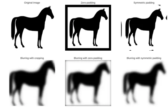
A first approach is to limit output region only to those pixels that are far enough from borders to have the convolution value exactly defined. In this way, output image have a smaller size than input image by the filter size minus one (“Blurring with cropping” in Figure 2.6).

The opposite method is to pad the input image, i.e. to add a border around the input image, so that pixels outside boundaries are actually defined. There are different methods to establish the value of those pixels.

The simplest one is to add zeros (“zero-padding”) outside the image. This approach is useful if the signal is supposed to go to zeros outside the region where it is defined. A variation is to pad with the supposed value, different from zero. For any variation, many discontinuities are created at borders. This method can create dark borders around convolved image as seen in Figure 2.6.

If the signal is supposed to be periodic, the “wrap-padding” will add paddings that are copies of the image on the other side of the axis, like a modulo operation on the position. This method also creates discontinuities.

Finally, a common approach with real-world image is the “symmetric-padding”, where the padding is a reflection with respect to the border. Discontinuities of the first deriva-tive are created at borders but this approach usually creates nice-looking borders on images. Original Image Blurring with cropping Zero­padding Blurring with zero­padding Symmetric padding Blurring with symmetric padding

Figure 2.6: Illustration of several kind of padding and the result of a convolution with a Gaussian blurring filter.

CHAPTER

3

GPU Implementation of Scattering

Convolutional Networks

One of the main purpose of this thesis is to implement the scattering network algorithm with a code that can run efficiently on a GPGPU.

The planning of the code has been guided by some objectives.

First of all, the implementation needed to be easy and fast to prototype. At the same time, high performance were required to obtain interesting results. Therefore the Python language has been chosen for its interpreted scripting nature that allows to prototype fast, the generous number of highly optimized, open source modules, and the previous experience of the author with this programming language. For the GPU side, CUDA[18] framework has been chosen to perform the parallel computations.

The desired code would have been packegable as a Python module to allow distribu-tion and reuse of the code. With this idea, the API of the module should have been as simple as possible, giving to the module the hard work of handling complex phases of the overall method.

Lastly, the complete module should produce results compatible with the Matlab code published by [3], to allow those who already use that implementation to switch seamlessly to the parallel high performance version.

This chapter begins with an overview of the world of computing on GPU, followed by the review of some software tools used in this work. After that, the development history of the produced software is described. Finally, compatibility and performance tests results are exposed.

3.1

_{GPU computing with CUDA}

Last decade have seen a tremendous increase of GPUs performance. As the name say, Graphics Processing Units arise from the demand of specialized chips to perform graphics computation. However, since the advent of frameworks like CUDA and OpenCL, GPU could be used for general purpose computing, speeding up computations of scientific research, engineering, medicine and other fields. The power of GPUs comes from the massively parallel computing that can be performed on these devices.

We will go into details of the CUDA framework, that is used in this work to efficiently parallelize the scattering network algorithm.

In CUDA, the parallel portion of the application is called kernel. Multiple instances of a kernel can be executed concurrently and each instance is called a thread. Threads are organized in blocks, a 1- 2- or 3-dimensional group of threads. Blocks are also organized in a grid. Each level of this hierarchy is executed on the respective hardware level. A CUDA-capable GPU can execute one or more grids of blocks. On the GPU, many Streaming Multiprocessors (SMs) handle the execution of the blocks. SMs are composed of many CUDA cores, the base ALU of a GPU. Each thread is run on a CUDA cores.

Therefore parallelization happens at thread level. Each thread run the same portion of code, but can elaborate different data. For example, let’s consider the element-wise sum of two vectors on N elements each. A 1-D block of N threads can be launched and every thread will add together one couple of elements of the vector. This kind of parallelization is called SIMT (Single Instruction Multiple Threads),

Figure 3.1: Grid of thread blocks. From the Cuda Programming Guide [19]. Multiple operations on a set of data can be chained by concatenating many kernels. If flow of input data is continuous, it can be considered a stream and all kernels can

run in parallel to perform operations on every item of the stream. This approach of performing parallelization is called stream processing and allows to achieve simple form of parallelization.

Parallel computation can be executed from a serial code running on the CPU through the CUDA API.

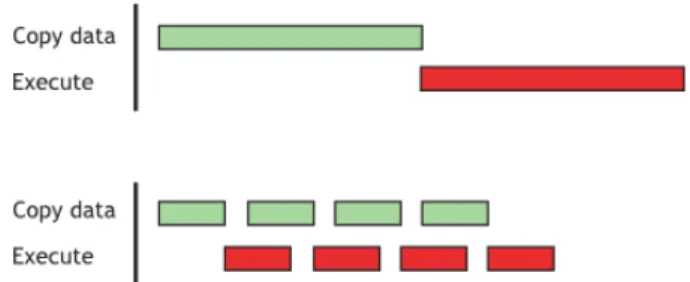
It’s worth pointing out some downsides of computing on GPU. First of all, CPU and GPU usually use different hardware memories, therefore memory copy must be performed at the beginning of the computation to move data from RAM to GPU memory and at the end to get results back to RAM. This copy can take a non negligible time, thus computing on GPU is profitable only if the speedup obtained by the parallelization is enough to ignore the transfer time. A second important point is that GPU architecture have an intrinsic high latency to start computing a thread but can achieve higher throughput compared to CPU. A common solution to both this problem is an efficient application of the stream processing paradigm to overlap memory copies and computations.

Figure 3.2: A sequential approach (top) and the overlapping of copy of data and thread execution (bottom). Latter approach can speedup execution. From the Cuda C Best Practices Guide [20].

Standard CUDA API are available in C, but bindings and wrappers for many different languages are available.

3.2

_{Software Tools}

Python ecosystem is rich of modules for almost any application. Many of them present core functions written in a compiled language and offer a Python interface to those functions. This method allows to achieve high computational efficiency despite using a simple and flexible interpreted language.

In this work, high performance have been looked for in four main modules: Numpy, PyCuda, Scikit-Cuda and OpenCV.

3.2.1 Numpy

Numpy [21] is a Python package for scientific computing that expose a powerful N-dimensional array object that can be used to perform most common and advanced mathematical operations between arrays. The core of the module is written in C to achieve high performance while exposing a simple interface in Python.

3.2.2 PyCuda

PyCuda [22] package gives access to Nvidia’s CUDA [18] API. The package can be used in two primary ways.

The first is to use the GPUArray1 _{object that exposes an interface like Numpy’s}

“ndarray” but stores and compute data on the GPU. Most common methods of Numpy are reimplemented in GPU code to take advantage of parallel architectures. For example, all point-wise operations (e.g. abs, sin, cos, ... ) and simple scans/reductions (e.g. min, max, sum, ...) are readily available. PyCuda will handle seamless all operations required by the CUDA API, like instantiating the context, moving data from RAM to GPU memory, creating and running CUDA kernels and getting back results to CPU memory. Instant benefits are usually obtained for large arrays.

The other way to use the module is to write custom CUDA kernels. This approach is suggested to developers that already know how to write own code for GPU but that wants to use a convenient and fast framework that handles all the background work and that allows to concentrate on the actual computing code. In particular, GPUArray’s ElementWiseKernel object allows to create a kernel that runs a user-defined operation on every element of the array. PyCuda will handle automatically the JIT (just-in-time) compilation of the kernel, its launch with suitable grid-size and block-size and eventual for-loops within the kernel around the code to achieve optimal performance. At necessity, all CUDA’s driver API are available to perform more sophisticated tasks.

3.2.3 Scikit-Cuda

Scikit-cuda[23] is a wrapper to many functions of CUDA, cuBLAS, cuFFT and cu-SOLVER libraries. It allows to run functions defined in those libraries directly in Python with the help of PyCuda to handle the movement of data to/from the GPU. In this work

it has been used primarily for the cuFFT binding. cuFFT 2 is a library that provide an

interface to compute FFTs on NVIDIA GPUs. Because the FFT is in operation that can be greatly parallelized, GPUs can yield to important benefits in terms of execution time.

1

https://documen.tician.de/pycuda/array.html Accessed on 11/14/2016.

2

3.2.4 OpenCV

The most famous library for computer vision is OpenCV [24]. Its Python bindings has been used in first revisions of the code to perform mainly the symmetric padding. This operation was seen to be faster with this library than the Numpy implementation.

During the development, though, the latest version of the library (v 3.1.0) was used to handle images from the loading, saving, resizing and color converting.

3.3

_Development

The GPU implementation was developed by writing a prototype of the software and iteratively enhancing it by fine-tuning slowest parts. In the history of this process, three main revisions of the software are reported below to disclose encountered problems and solutions found.

3.3.1 First implementation

The first implementation of the code was based on a quasi-straightforward conversion from Matlab code to Python code with the use of GPU capabilities only on the critical step of the convolution in the Fourier space.

The algorithm worked layer-wise, iterating over each layer m to compute new coeffi-cients SJ[p]x and U [p]x.

It was clear that almost always at each layer there were multiple signals U [p] with the same size (possibly reduced from the original size by the subsample steps). Since

cuFFT implementation is known to work good in batches of signals of same shape3_{, this}

feature was exploited.

At each layer, the algorithm searches for paths whose size is the same and it groups them. Next, each group of signals is elaborated sequentially. Every signal in the group is padded and then they are stacked in a 3-dimensional Numpy array that is copied to GPU in a GPUArray. This array is fed into the cuFFT’s FFT routine to compute the transformation in batch. Then the history of every signal is checked and they are multiplied by the appropriate filters, saving results in a new 3-d GPUArray. This array of filtered spectrums is inverse transformed still in batch to obtain wavelet transformed signals. Always on the GPU, the module operation is performed element-wise. Finally, data are copied back from GPU to CPU memory where unpadding and downsample operations were performed.

Performance of this first version were not great, with a very little speedup compared to Matlab code. Most of the time was spent transferring data to and from the GPU and launching kernels. Indeed, GPU functions need to have enough computational work to

3

execute so that the overhead time, required by the operation of launching computation and the time-extensive memory copy, is negligible with respect to the actual computa-tion time. The proposed algorithm requires plenty of memory movements so the GPU capabilities are not used at the maximum of their possibilities. This is due to the fact that there were not enough signals of the same shape in each layer to elaborate together. Nevertheless, this implementation did not require any knowledge of GPU program-ming, because the only encounter with GPU-related functions is the necessity to call functions to move memory to and from the GPU. Thanks to the Python modules used, this is operation was very easy and others functions ran on the GPU had same syntax of ones that would have ran on the CPU.

3.3.2 Second Revision

The second revision of the code took advantage of the observation that the scattering network graph did not need to be forcingly walked layer by layer, but that each path can go on alone, with the only necessity to have completed all paths at the end of the execution.

With this consideration, it can be seen that graph could be walked in such a way that all intermediate signals with the same size are computed at the same iteration. This is accomplished by performing scattering convolution always on those image that have the bigger shape, that are those with the smallest overall downsample rate. If the graph is represented such that filters are scattered left to right according to the increasing j, it’s clear that the graph is walked “diagonally”, from top left to bottom right.

The implemented algorithm creates and keep a queue of intermediate signals, i.e. incomplete paths. It iterates until there are no more elements in the list by first searching the maximum shape of signals in the list and then grouping all signals with that shape. Those signals are also removed from the list. Then the appropriate filter size for this shape is selected from pre-calculated filters and signals are symmetrically padded and moved to the GPU in stack as in the previous version of the code. The stack is then transformed to the Fourier space and after that each spectrum is point-wise multiplied with appropriate filters. Like before, signals are transformed back in the spatial space with the batched IFFT and the modulo is applied point-wise. The next step is to copy back filtered signals to CPU, where unpadding and downsample is applied. For each signal in the group, if it ended its path it is copied to an output stack, otherwise the intermediate output is added back to the queue list, and another iteration is performed. As they are usually not needed for subsequent analysis, this approach doesn’t save intermediate results U [p].

This evolution of the algorithm allowed to obtain a first interesting speedup relative to CPU implementation. This is achieved by the more effective computation of the FFT and IFFT, that are now executed with the largest possible batches of signals of the same shape. Some memory problems arose because with some combinations of J , L and

original image shape, in the firsts steps of the processing the memory required for the IFFT was too large to fit in the not-so-big memory of GPU, especially low-end ones. To mitigate this problem, a solution was found by limiting the size of the batch of signals simultaneously computed: for each group, if its total number of pixels exceed a defined threshold, the group was splitted. This allows to use most of the available GPU memory without having fails during allocation.

Now that the convolution heavy computation is totally delegated to the GPU, the main bottleneck of the process were other operations ran on the CPU, together with the need to move memory to and from GPU too frequently. In particular, it was seen from profiling the code that the padding, unpadding and downsample steps computed on the CPU took about 20 % of the overall execution time.

3.3.3 Latest release

The further and last evolution of the algorithm solved bottlenecks of the last revision and achieved highest performance.

This version is based on the good approach of crossing the scattering network di-agonally, but it also delegate to the GPU all signals computations by creating custom CUDA kernels and managing efficiently the memory allocation and copy.

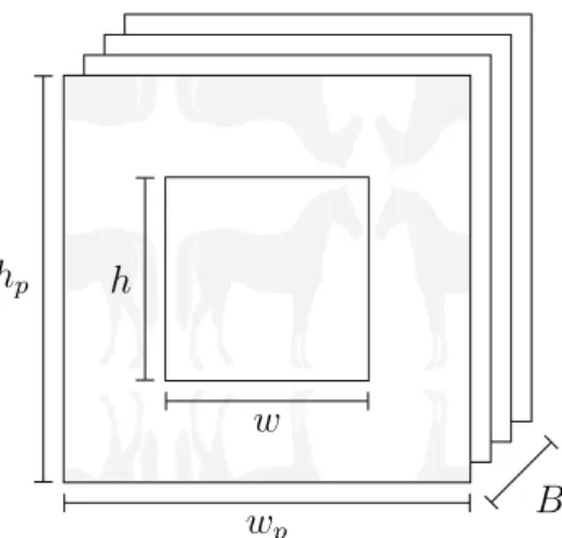
In details, the concept of “signals container” is introduced: this is a Python object that contains a GPUArray who store a stack of signals with the same shape (like the concept of groups in previous revision). Moreover, the shape of the GPUArray is such that it can store also the correct padding that is required to handle border problems of

convolution. Overall, the GPUArray is 3-dimensional, with a shape given by (B, wp, hp)

where B is the number of signals that will be stored, hp and wp the height and width of

the padded version of the signals (Figure 3.3).

A set of containers is created at initialization time, one for each downsample scale that will be met during computation of the scattering network (basing on hyper-parameters M , J , L and image shape). An additional container is prepended to the set to store the original image, that is immediately copied to GPU.

The algorithm basically iterates over the set of containers.

For each containers it pads the image with a custom CUDA kernel created with the “ElementwiseKernel” class offered by “PyCuda”, so it is run element-wise over all pixels of signals and padding in the containers. For each pixel, it finds the location on the original image coordinates: if the current pixel is already one of the original image, it is copied in-place; otherwise, if it is one of the border, the corresponding pixel mirrored on the border is copied. This method allows to efficiently and parallely apply the symmetric padding directly on the GPU, without requiring any copy to CPU. No already existing library with this functionality was found, so in previous versions of the code it was required to move image back on CPU also to perform this operation with OpenCV’s copyMakeBorder.

wp

hp

w h

B

Figure 3.3: Illustration of a “signals container”. A stack of B signals is saved in a 3D

GPUArray. The signal size is w × h, but a larger space wp× hp is allocated to hold the

symmetric padding.

Next, all signals in the container are transformed to the Fourier space in batch. Filters are then loaded, and another custom CUDA kernel is called on each filter to be multiplied for required signals. This allows to load pixels of each filter in GPU registers only once for all the signals that requires that convolution.

Then the IFFT function is called always in batch to transform back signals.

The latest custom CUDA kernel handles operations of unpad, downsample and appli-cation of the modulus. This phase is preceded by a preparation step where it is created a list of associations between each convolved signal, related downsample factor and des-tination container. Then, for each desdes-tination container, the custom CUDA kernel is run. Basing on information related to source and destination shape, source and desti-nation padding and downsample, it maps every source pixel to appropriate destidesti-nation pixel while applying modulo operation. Therefore the computation of the modulo is performed only on useful pixels, while others are discarded.

When the iteration on the last container is concluded, its data (that at this point

are scattering coefficients SJ[p]) are copied back to the CPU memory and computation

is done.

Another feature of this implementation is that allocated GPU memory for containers can be reused for subsequent transformations through the scattering network, so next runs will not have to wait the time required for the memory allocation.

The realization of this approach definitely required CUDA programming skills and knowledge on GPU coding best practices. Custom CUDA kernels are built exactly to optimize the scattering network algorithm, so the implementation is ad-hoc. Previously cited Python modules are used anyway for complex tasks, like the FFT/IFFT transform and the possibility to create effective and simple element-wise kernels. Without those

modules, the time required to write the code and its length and complexity would have been certainly higher.

3.4

_{Packaging and distribution}

Last version of the software was packaged as the Python module scatnetgpu. The module have several dependencies:

q _{numpy>=1.11.0 Python library for CPU numeric computations}

q _{scipy>=0.18.0 Python library used only to calculate the binomial coefficient}

q _{pycuda>=2016.1.2 Python library for heavy computations on the GPU}

q _{scikit-cuda>=0.5.1 Python library for the cuFFT wrapping}

q _{octave framework, oct2py Python library, Scatnet Matlab code} 4 _{required to load}

the filter creation function of the original Matlab code through octave (necessary as long as that part of the code is not ported to Python)

The main class available in the module is ScatNet. The class can be instantiated by passing parameters M , J and L of the required scattering network. The resulting object have the useful method transform that perform the scattering network transformation of a given image (represented by a Numpy ndarray). This method takes care of creating filters if they are not already present in cache, then it performs the transformation and returns the result in form similar to the one of the Matlab code. If a batch of images needs to be transformed, the method batch transform takes care of looping over the batch. If given ndarray have 3-dimensions, the last one is considered to represent channels (e.g. RGB, HSV, ...). Every channel is transformed alone, and resulting representations are concatenated.

An additional utility function, stack scat output, takes the transformed represen-tation and returns a 3-dimensional ndarray where each scattering output is stacked in the first dimension, in addition to a list of meta-data to recognize the paths of the net-work. This was useful for the later classification procedure, because the order of the output is not important in this task.

The source code has been released open-source under MIT License and it’s available at: https://github.com/oinegue/scatnegpu. From the link, the code can be reviewed, downloaded, easily installed and modified. In this way, I hope to make available to other researchers a fast (as further discussed in Section 3.6) implementation of the scattering network algorithm, in order to continue studies for new uses of this representation and to permit the realization of real-time applications.

4

3.5

_{Compatibility Tests}

The GPU implementation was tested to be compatible with the reference Matlab code. Tests were performed at many levels of aggregation, to check that any combination of parameters leaded to compatible scattering coefficients in output.

Firstly, outputs of the GPU code and the Matlab code were compared pixel-by-pixel. We are looking at the result of a machine computation, thus the analysis must take in account that number are expressed in a floating point representation, as expressed in the standard [25]. In this specific case, all computations are performed in single precision, so each value is stored in memory with 32 bits.

The absolute difference |x1− x2| between two machine numbers x1 and x2 can show

qualitatively if the results are nearly correct. To quantify the magnitude of the eventual difference, it’s important to validate discrepancies of the results with respect to the capabilities of the single precision floating point representation used.

A generic approach to this problem is to use the concept of Unit in Last Place (ULP) [26]. Given a floating point number x whose exponent is E, it is defined U LP (x) =

(0.0...01)2× 2E. More intuitively, the ULP is the gap between x and its very next larger

floating point number. Therefore a method [27] to evaluate the difference between two floating point numbers is to count how many ULPs there are between them. This count is usually called NULP (Number of ULPs).

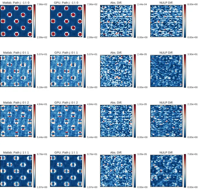
Figure 3.4 represents an example of the tests. It can be observed that both version appears qualitatively similar in first two columns. Nevertheless, the absolute difference is non zero almost everywhere. This may be due to the different implementations of functions like the FFT/IFFT, to round-off error of the single precision floating point representation used and to its propagation with the particular order of the operations performed in the final revision of the algorithm. However, the NULP difference exposed in the last column is limited. Considering the big number of operations involved in the scattering network base algorithm, this result is considered acceptable. Therefore, standing to this first result, the two algorithms are compatible.

The study followed by analyzing the biggest NULP difference in the output signals of each path of a scattering network. Box plot of Figure 3.5 is built by computing the maximum NULP difference of each path of a scattering network and collecting this result for 100 different input images from the textures dataset used in Chapter 5. It’s clear that even with a large set of images, the NULP difference between the two algorithms remains low. Some outlier values reach higher difference. It was observed that these discrepancies are higher in regions of images that are nearly black. This may be due to round-off errors that for small numbers are amplified during the FFT/IFFT.

Compatibility has been tested over a range of different image sizes and scattering network configurations, to check if the implementation was correct. The Figure 3.6 show one of the tested scattering network configuration. It can be observed that the maximum

Matlab. Path j: ­1 l: 0 2.99e+02 7.96e+02 GPU. Path j: ­1 l: 0 2.99e+02 7.96e+02 Abs. Diff. 0.00e+00 2.44e­04 NULP Diff. 0.00e+00 8.00e+00 Matlab. Path j: 0 l: 1 5.18e+00 5.07e+01 GPU. Path j: 0 l: 1 5.18e+00 5.07e+01 Abs. Diff. 0.00e+00 2.48e­05 NULP Diff. 0.00e+00 3.90e+01 Matlab. Path j: 0 l: 2 5.44e+00 4.84e+01 GPU. Path j: 0 l: 2 5.44e+00 4.84e+01 Abs. Diff. 0.00e+00 1.91e­05 NULP Diff. 0.00e+00 2.20e+01 Matlab. Path j: 1 l: 1 1.97e+00 9.76e+01 GPU. Path j: 1 l: 1 1.97e+00 9.76e+01 Abs. Diff. 0.00e+00 3.05e­05 NULP Diff. 0.00e+00 7.00e+01

Figure 3.4: Representation of the compatibility of the outputs for a polka dot image. Original image size was 128 px × 128 px. Scattering network parameters were M = 2, J = 2, L = 2. From left to right: output of Matlab code, output of GPU code, pixel-wise absolute difference, NULP difference. From top to bottom, different paths of the scattering network are shown.

j: ­1 l: 0 j: 0l: 1 j: 1l: 1 j: 2l: 1 j: 0,1l: 1,1 j: 0,2l: 1,1 j: 1,2l: 1,1 Scattering Path 0 20 40 60 80 100 nULP Difference

Figure 3.5: Maximum NULP difference between Matlab and GPU implementation for each scattering path of a network with J = 3 and L = 1. 100 repetitions were run with different images. 0 100 200 300 400 500 Size (px) 0 100 200 300 400 500 600 Max NULP Difference

Figure 3.6: Maximum NULP difference between Matlab and GPU implementation for increasing image size with J = 3 and L = 1. 10 repetitions were run for each size. Median value is displayed as a solid line.

NULP difference increases with the image size. It’s hard to define an objective threshold for the compatibility of the results of a floating point calculation. Nevertheless, most of the values stay below 500 NULP of difference. This value seems to be a good result

compared to the 224 values that are representable with the same exponent of a single

precision floating-point number.

If further accuracy is needed, the causes of the incongruity should be searched in every function used in the algorithm, by comparing Matlab results with Python/CUDA results. Moreover, the particular order of functions in the algorithm could lead to different round-off errors that accumulates to create the different results.

3.6

_Performance

Execution times of the scattering network algorithm were compared for both the GPU implementation and the Matlab code running on the CPU. Tests were performed on the following machines:

lenome notebook A personal notebook with a discrete graphic card

q _{Model: Lenovo Flex 2-14}

q _{CPU: Intel(R) Core(TM) i5-4210U CPU @ 1.70GHz}

q _{RAM: DDR3 1600 MHz 8 GB}

q _{GPU: Nvidia GeForce 840M}

– Architecture: Maxwell – CUDA cores: 384 CUDA – Max Clock: 1.12 GHz – Memory: DDR3 4 GB q _{OS: Ubuntu 15.10} q _{CUDA version: 7.0} q _{Matlab version: R2016b} q _{Octave version: 4.0.0}

phantom desktop An assembled desktop used for basic machine learning tasks

q _{CPU: AMD FX(tm)-8350 Eight-Core Processor}

q _{RAM: DDR3 1866 MHz 16 GB}

q _{GPU: Nvidia GeForce GTX 960}

– CUDA cores: 1024 CUDA – Max Clock: 1.29 GHz – Memory: GDDR5 2 GB

q _{OS: CentOS 7.2.1511}

q _{CUDA version: 7.5}

titano workstation An assembled workstation used for heavy machine learning tasks

q _{CPU: Intel(R) Core(TM) i7-5930K CPU @ 3.50GHz}

q _{RAM: DDR4 2133 MHz 32 GB}

q _{GPU: Nvidia GeForce GTX TITAN X}

– Architecture: Maxwell – CUDA cores: 3072 CUDA – Max Clock: 1.08 GHz – Memory: GDDR5 12 GB

q _{OS: Ubuntu 14.04.5}

q _{CUDA version: 7.5}

First of all, the execution time of the mere transformation function was measured (ScatNet.transform for Python, scat for Matlab). Test was performed by running the function in loop for 10 executions and measuring the mean time required for each execution. The measuring was repeated 5 times and best result was reported to mitigate possible breaking due to the operating system. Several combination of image size S, filters scales J and rotations L were tried (an image of size S is intended to be a gray-scale square image of size Spx × Spx).

In Python, time was measured with the time.clock() function 5. In Matlab, the

couple of functions tic; <code>; tac; was used 6_.

Figure 3.7 and Figure 3.8 reports measured performance of two extremities of param-eters combinations, respectively a small network with J = 3, L = 4 and a large network with J = 5, L = 8. Different image size were tried, from S = 32 to S = 1024 at steps of ∆S = 32. In both cases, the same overall trends are observed: GPU code is faster than CPU code, more powerful GPUs scores faster results, Octave interpreter is slower than Matlab interpreter.

Starting the analysis from the last point, the speed-up of Matlab with respect to Octave is up to 4 times for small images and for both parameters configurations. Speedup

5

https://docs.python.org/2/library/time.html#time.clock. Accessed on 11/18/2016.

6

https://it.mathworks.com/help/matlab/matlab_prog/measure-performance-of-your-program.html. Accessed on 11/18/2016.

32 64 96 128 160 192 224 256 288 320 352 384 416 448 480 512 544 576 608 640 672 704 736 768 800 832 864 896 928 960 9921024 Size (px) 10­2 10­1 100 101 Time (s) 60ms 49ms59ms68ms 80ms92ms102ms 141ms 230ms215ms252ms206ms252ms 393ms409ms404ms486ms 847ms 601ms 1.0s869ms 676ms 1.1s 851ms1.0s 1.4s 996ms 1.4s1.6s 2.3s 1.3s 1.4s 219ms215ms238ms270ms296ms317ms285ms322ms 354ms356ms413ms400ms479ms542ms 595ms607ms606ms 895ms_759ms1.0s 1.0s877ms 1.2s 995ms1.2s 1.5s 1.2s1.4s 1.7s2.0s_{1.5s 1.6s} 26ms27ms32ms35ms 42ms54ms56ms 77ms89ms85ms 116ms115ms123ms 171ms191ms181ms191ms 266ms364ms327ms357ms295ms 420ms 351ms 602ms536ms_447ms747ms660ms742ms618ms 966ms 16ms16ms18ms23ms21ms24ms24ms 28ms30ms30ms37ms37ms38ms 48ms53ms49ms52ms 68ms79ms87ms 100ms 72ms 108ms 82ms 128ms143ms 104ms 155ms170ms185ms_139ms199ms 16ms17ms18ms20ms19ms 24ms23ms27ms27ms28ms30ms30ms26ms30ms34ms33ms31ms 49ms50ms 68ms76ms 46ms 82ms 49ms 89ms 137ms 99ms127ms 168ms191ms 128ms165ms

Performance Comparison with M:2 J:3 L:4

Implementations

Figure 3.7: Execution time of the scattering network transform with M = 2, J = 3 and L = 4 at different image size S.

32 64 96 128 160 192 224 256 288 320 352 384 416 448 480 512 544 576 608 640 672 704 736 768 800 832 864 896 928 960 9921024 Size (px) 10­2 10­1 100 101 Time (s) 478ms525ms572ms658ms 724ms817ms875ms 1.5s 1.4s 1.3s 1.4s 1.6s1.7s 1.9s 2.3s 2.3s2.9s 2.8s 3.1s 3.5s4.1s 3.9s 4.1s 4.5s 5.0s 5.3s6.8s 5.9s7.4s 6.6s 6.9s 8.3s 2.3s 2.3s 2.5s 2.5s 2.6s 2.5s2.9s 2.8s 3.2s 3.1s 3.4s 3.5s 3.5s 3.7s4.2s 4.5s 4.6s 4.6s 4.9s 5.6s5.8s 6.0s 6.2s 7.2s 7.1s 7.7s8.6s 7.9s 9.3s 9.1s 9.3s 10.3s 72ms79ms 131ms163ms 201ms232ms 278ms333ms 403ms454ms 701ms614ms720ms848ms 1.2s 947ms 1.4s 1.2s 1.3s1.4s 2.1s 1.7s2.1s 2.6s 2.2s 2.4s 3.3s 51ms52ms64ms68ms 75ms83ms94ms102ms 114ms125ms 164ms158ms168ms198ms 252ms228ms305ms281ms 40ms44ms52ms54ms58ms 62ms66ms69ms67ms79ms 100ms86ms125ms 154ms187ms169ms 252ms227ms231ms247ms 370ms 291ms355ms426ms391ms432ms 539ms484ms639ms550ms693ms704ms

Performance Comparison with M:2 J:5 L:8

Implementations

Figure 3.8: Execution time of the scattering network transform with M = 2, J = 5 and L = 8 at different image size S.

32 64 96 128 160 192 224 256 288 320 352 384 416 448 480 512 544 576 608 640 672 704 736 768 800 832 864 896 928 960 9921024 Size (px) 0 1 2 3 4 5 6 7 8 9 10 11 12 13 14 15 16 17 18 19 20 21 22 Speedup

Speedup relative to matlab_lenome with M:2 J:3 L:4

Implementations

Figure 3.9: Speedup of the GPU implementation with respect to Matlab version for the scattering network of Figure 3.7

32 64 96 128 160 192 224 256 288 320 352 384 416 448 480 512 544 576 608 640 672 704 736 768 800 832 864 896 928 960 9921024 Size (px) 0 1 2 3 4 5 6 7 8 9 10 11 12 13 14 15 16 17 18 19 20 21 22 Speedup

Speedup relative to matlab_lenome with M:2 J:5 L:8

Implementations

Figure 3.10: Speedup of the GPU implementation with respect to Matlab version for the scattering network of Figure 3.8

drops for big images, scoring similar results for the small network and a little speedup for the large network. Better performance may be due to many optimizations of the Matlab environment not present in Octave. For example, it was observed that many cores were busy during Matlab execution while Octave run occupied only one core. This could mean that in Matlab some functions used in the algorithm are parallelized (like the FFT or matrix multiplications). A further study of the differences between the two environments is beyond the scope of this work and then, because of the higher performance, subsequent comparison will be based only on time measures in the Matlab environment.

Performance improvements of the GPU implementation relative to Matlab code de-pends obviously on the specific GPU. In Figures 3.9 and 3.10 it can be seen that for the entry-level GPU of lenome notebook, the speedup is around 2× for the small network and peaks at more than 6× for the large one and small images, decreasing again to 2× for bigger images.

Medium range GPU of phantom desktop have better performance. The small net-work configuration shows a speedup from 3× up to more than 10×. Speedup increases with image size, showing that the potential parallelism of the GPU is exploited when occupancy of the cores is high. The big network shows a mean performance increase of about 10×, with a peak when the Matlab code show an important slow-down at around S = 256 px.

Top-level GPU of titano scores top performance with a general trend similar to that of the previous graphic card, but with an additional speedup relative to the Matlab code, up to 17× for the small network and 21× for the bigger one. Again, the computational capabilities of these devices is not completely accessible for low complexity tasks (small network and image sizes), but the performance gain is important for heavy calculations. Looking at absolute values, the new GPU implementation can reach nearly real-time performance in several combinations of parameters. For big networks, mid/high GPUs scored less than 100 ms (10 FPS) for images up to 256 px. This result can be useful for practical applications where a high rate of processed images is needed, like in industrial environments or video processing.

All curves presents spikes at certain image sizes. They are due to the performance of the FFT and IFFT algorithm at different signal sizes. In fact, standing to the

documen-tation of cuFFT7, the implementation is optimized for image sizes that can be factorized

as powers of small prime numbers, i.e. S = 2a₃b₅c₇d_{. If the size can not be factorized}

in this way, more computation are required and execution time increases. Figure 3.11 shows the described behaviour: time required to run an FFT varies greatly even chang-ing image size of only 1 px. Due to the paddchang-ing, this situation can happen despite the initial image size. A better implementation of the algorithm could estimate the optimal padding for this requirement. This optimization has not been implemented in the last revision of the software because filters creation is still based on the original Matlab code.

7

0 200 400 600 800 1000 Image Size (px) 0.00 0.01 0.02 0.03 0.04 0.05 FFT Time (s)

Figure 3.11: Time required to run a single 2D FFT transform on a square gray-scale image with cuFFT through Python bindings offered by Scikit-Cuda (averaged over 10 runs).

A final note is that many points are missing in the big network chart, at large image sizes, in the GPU curves of lenome and phantom. Memory required to perform the (I)FFT depends heavily on the image size and for some “unlucky” dimensions it could

be as large as 8 times the memory of the original signal 8_{. The (I)FFT in the algorithm}

is run in batches, so the memory requirement may be too large to be allocated on the limited memory of the GPU and so execution will fail for this sizes. Two methods are possible to bypass the problem. The first is to limit the number of signals in the batch and instead run multiple batches of (I)FFT. The second method is to split the image in multiple patches, perform the scattering network transform on each patch and finally recombine the outputs. The latter approach generalize better for very large images, but requires attention to treat correctly the behaviours at borders.

Every code enhancement was guided by the time profiling of the previous version. Each macro block of the algorithm was enclosed in a couple of stopwatch timers to measure how much time was spent in each part of the code. In the following, the time profiling of executions of the latest code on phantom is shown.

Table 3.1 reports the time profiling of a run of the small network of Figure 3.7 launched on phantom with image size 512 px. First observation is that more than half of the time is used for the entire convolution operation (FFT, Element-wise Multiplication, IFFT), that involves 67 % of the total computation. Surprisingly, the copy of the filters

8

0 20 40 60 80 100

Color Operation Percentage Time

IFFT 30% 20.8ms

FFT 22% 15.1ms

Filters copy CPU → GPU 18% 12.3ms

Element-wise Multiplication 15% 10.1ms

Unpad / Downsample / Modulus 7% 5.1ms

Symmetric Padding 3% 2.3ms

Containers Allocation 2% 1.1ms

Preparation 1% 0.6ms

Results copy GPU → CPU 1% 0.5ms

Image copy CPU → GPU 1% 0.4ms

Format Output Data 1% 0.4ms

Table 3.1: Time profiling of the Scattering Network algorithm on phantom’s GPU. Image size was 512 px × 512 px, parameters were M = 2, J = 3, L = 4. Number of scattering coefficients produced is 249856 Times averaged over 100 runs.

0 20 40 60 80 100

Color Operation Percentage Time

IFFT 40% 100.0ms

Filters copy CPU → GPU 24% 60.5ms

Element-wise Multiplication 18% 44.8ms

FFT 8% 19.1ms

Unpad / Downsample / Modulus 4% 9.1ms

Preparation 2% 5.7ms

Containers Allocation 2% 4.3ms

Format Output Data 2% 4.0ms

Image copy CPU → GPU 0% 0.5ms

Results copy GPU → CPU 0% 0.4ms

Symmetric Padding 0% 0.2ms

Table 3.2: Time profiling of the Scattering Network algorithm on phantom’s GPU. Image size was 512 px × 512 px, parameters were M = 2, J = 5, L = 8. Number of scattering coefficients produced is 174336. Times averaged over 100 runs.

0 20 40 60 80 100

Color Operation Percentage Time

Element-wise Multiplication 44% 27.1ms

IFFT 14% 8.5ms

FFT 11% 6.7ms

Preparation 10% 6.0ms

Format Output Data 7% 4.2ms

Containers Allocation 6% 4.0ms

Unpad / Downsample / Modulus 6% 3.4ms

Filters copy CPU → GPU 2% 1.5ms

Symmetric Padding 0% 0.2ms

Image copy CPU → GPU 0% 0.2ms

Results copy GPU → CPU 0% 0.1ms

Table 3.3: Time profiling of the Scattering Network algorithm on phantom’s GPU. Image size was 32 px × 32 px, parameters were M = 2, J = 5, L = 8. Number of scattering coefficients produced is 681. Times averaged over 100 runs.

from CPU to GPU is another important part of the transformation, that spends nearly one fifth of the time moving filters. This is because filters in the Fourier space occupy lot of memory and the memory transfer speed to and from the GPU is still one of the main bottleneck of GPU programming.

It would be interesting to evaluate the possibility to create filters directly on the GPU to avoid this memory copy, but the trade-off with the computation time required for their creation may not worth the hassle.

At the opposite, operations like symmetric padding, unpadding, downsample and modulus benefit a lot of the custom implementation in CUDA kernels. Their overall contribution is about 10 % and hence does not influence essentially the overall timings.

The container allocation operation refers to allocating memory on the GPU device to store intermediate results of the algorithm. If a batch of images needs to be transformed, this operation is required only once because allocated memory would be reused, saving a bit of time.

An analogous operation with the filters copy was not possible because the whole filter bank is too big to be stored on the GPU when other memory intensive operations like FFT/IFFT need to be performed.

Format Output Data represents the operation of organizing results like original Mat-lab code does and Preparation is a group of operations that arrange the environment for the execution of the algorithm. Finally, transferring input image from the CPU to GPU and getting scattering coefficients back are cheap operations because the size of the data is small.