Aerodynamics of rotating wheels: analysis of different modelling approaches

Politecnico di Milano

Scuola di Ingegneria Industriale e dell’Informazione

Corso di Laurea Magistrale in Aeronautical Engineering

specializzazione Propulsione

Tesi di Laurea Magistrale

Aerodynamics of rotating wheels:

analysis of different modelling approaches

Autore:

Enrico Panunzio

Matricola 899508

Relatore:

Contents

Introduction 14

1 State of art 17

1.1 The simplest case: 2D cylinder . . . 17

1.2 Wind tunnel tests . . . 18

1.3 CFD simulations . . . 21

1.3.1 Rotating model approach . . . 21

1.3.2 Shoulder type and hub influences . . . 25

1.3.3 Stationary vs rotating . . . 27

1.3.4 Steady vs unsteady . . . 28

1.3.5 Step contact patch . . . 29

1.3.6 Slick vs grooved . . . 29 1.3.7 Velocity comparison . . . 35 1.4 Author’s conclusion . . . 37 2 Governing equations 38 2.1 Navier–Stokes equations . . . 38 2.2 Discretization . . . 40 2.3 RANS equations . . . 43 2.4 Q criterion . . . 44 2.5 k–ωSST . . . 44 2.6 Rotating models . . . 45

2.6.1 Rotating wall velocity . . . 45

2.6.2 Moving Reference Frame . . . 46

2.6.3 Sliding Mesh . . . 49 3 Case setup 50 3.1 Geometry . . . 50 3.1.1 Wheel design . . . 51 3.1.2 Model preparation . . . 52 3.2 Meshing criteria . . . 53

3.2.1 Wind tunnel mesh . . . 54

3.3 Boundary conditions . . . 58

3.4 Turbulence model choice . . . 59

3.4.1 Case description . . . 60

3.4.2 Results . . . 62

3.4.3 Turbulence model conclusions . . . 70

3.5.1 Steady state simulations . . . 71

3.5.2 Unsteady simulations . . . 71

4 Results 73 4.1 In–depth analysis of wheel A simulations . . . 74

4.1.1 Steady state simulations . . . 74

4.1.2 Unsteady simulations . . . 84

4.2 Force coefficients comparison . . . 91

4.2.1 Wheel A . . . 91

4.2.2 Wheel B . . . 93

4.2.3 Comparison between wheel B and A . . . 94

4.3 Comparison between computational cost and time . . . 96

5 Conclusions 98 Future developments . . . 101

List of Figures

1 Graphical representation of the reference frame adopted in this work. . . 16 1.1 Stream lines and pressure distribution along a cylinder . . . 18 1.2 Main vortical structures produced by a wheel in contact with the ground [21]. . . 19 1.3 Values of the pressure coefficient along the centreline of the wheel [8]. . . 20 1.4 Ventilation moment for the slick pattern splitted between regions, for every

com-bination adopted, found by Hobeika and Sebben [14]. . . 23 1.5 Ventilation moments for the grooved pattern splitted between regions, for every

combination adopted, found by Hobeika and Sebben [14]. . . 24 1.6 Flow structures for the A2 rotating wheel; . . . 26 1.7 Centreline CP distribution of Fackrell’s test, transient and steady RANS

simula-tions [7]. . . 28 1.8 Total pressure contour plots along a normal plane at x/d=0.64 and on a plane

parallel to the ground at z/d=0.015, for two different step height: . . . 30 1.9 Section of the wheel, with its characteristic dimensions in millimeters [21]. . . 31 1.10 Representation of the MRF domain inside the wheel: it is marked in green on the

left picture, while it’s the ”A” region on the right [21]. . . 32 1.11 Combination of boundary conditions applied in the contact patch region [21]. . . 32 1.12 Centreline CPdistribution of Fackrell’s measurements, Lesniewicz simulation and

Mears’ test for the slick tyre [21]. . . 34 1.13 Centreline CPdistribution of Fackrell’s measurements, Lesniewicz simulation and

Mears’ test for the grooved tyre [21]. . . 34 1.14 Velocity vector for the slick tyre, on the left, and for the grooved tyre, on the

right. The area 1 represents a region of lower velocity; the area 2 underline the different vortex location; the area 3 shows the outwash behind the wheel caused by the fluid propagation along the grooves [21]. . . 35 1.15 Velocity – drag coefficient relation for grooved and slick tyre, according to the

driving speed found in European driving test cycle [20]. . . 36 3.1 Front and side views of the main features of wheel A, with the characteristic

dimensions. . . 51 3.2 Front and side views of the main features of wheel B, with the characteristic

dimensions. . . 52 3.3 Representation of the different regions. . . 53 3.4 On the left, the wheel without lateral grooves used to obtain the correct MRF

domain. . . 54 3.5 On the left, the feature edges of the cylinder were extracted. . . 55

3.6 Schematic representation of the tunnel blocks on the left and a close look to the resulting base mesh on the right. . . 56 3.7 The bounding boxes of the refinement regions 1, 2 and 3. . . 56 3.8 Layers coverage and levels obtained on the wheel; the most critical point are the

shoulders, especially next to the lateral grooves. . . 57 3.9 Graph that shows the convergence of the coefficients respect to a more dense mesh. 58 3.10 Representation of the computational domain; the green face is the inlet, the red

one is the outlet, the others are the wall with the slip condition. . . 59 3.11 A close look on the wheel portion, with its characteristic dimensions and the height

division in three main layers. . . 60 3.12 The unphysical flow field inside the domain while using the realizable k–ε model

with very low y+. . . 63 3.13 Comparison between the velocity magnitude field around the bump for the first

(the upper picture) and the fourth model. . . 63 3.14 Graph comparison of wall shear stress magnitude, pressure, y+ and velocity profile

between the three turbulence models for very low y+ values. . . 64 3.15 Flow field velocity magnitude view and pressure distribution along the bump for

the Spalart–Allmaras model with no–layers mesh. . . 65 3.16 Flow field velocity magnitude representation around the bump, respectively for: . 66 3.17 Graph comparison of wall shear stress magnitude, pressure, y+ and velocity profile

between the three turbulence models respect to the reference case for high y+ values. 66 3.18 Graph comparison of wall shear stress magnitude, pressure, y+ and velocity

pro-file between different layers configuration for the realizable k–ε, respect to the reference case. . . 68 3.19 Graph comparison of wall shear stress magnitude, pressure, y+ and velocity profile

between different layers configuration for the k–ω SST, respect to the reference case. 69 3.20 Value of the y+ field on the front wheel surface, using the k–ω SST turbulence

model and a steady state simulation. . . 70 4.1 Velocity magnitude field representation over a longitudinal slice at Y = 0.0125 m,

that cuts one of the rain grooves, of the first and second combination respect to the sliding mesh approach. . . 75 4.2 Velocity magnitude field representation over the centreline slice, respect to the

sliding mesh approach, for the steady state simulations; the minor wake of the reference case is emphasized by the white circle. . . 76 4.3 A close–up view to the low velocity region located in the upper back of the wheel

for the steady state simulations respect to the reference one. . . 77 4.4 A close–up view to the thin, separated wake presents only in the reference case,

compared to the steady state simulations; the circles emphasize the different shapes of the wake. . . 77 4.5 Glyph representation inside the lateral grooves located approximately at θ = 0◦_;

their orientation is in accordance to the velocity direction and their colours repre-sent the velocity along the Y axis; the frame of reference is in accordance to figure 1. . . 78 4.6 Glyph representation inside the lateral grooves located approximately at θ = 290◦_;

their orientation is in accordance to the velocity direction and their colours repre-sent the velocity along the Y axis; the frame of reference is in accordance to figure 1. . . 79

4.7 Velocity magnitude representation along the longitudinal plane located at Y = 0.075 m, which cuts all the lateral grooves. . . 80 4.8 Side view of the isosurfaces extracted from the Q criterion, applied to the mean

velocity for all the steady cases and compared with the sliding mesh approach at 1.6 s, with Q = 5 ∗ 103_{. . . . 81}

4.9 Back view of the isosurfaces extracted from the Q criterion, applied to the mean velocity for all the steady cases and compared with the sliding mesh approach at 1.6 s, with Q = 5 ∗ 103_{. . . . 82}

4.10 Close–up on the top pf the wheel of the isosurfaces extracted from the Q criterion, applied to the mean velocity for all the steady cases and compared with the sliding mesh approach at 1.6 s, with Q = 5 ∗ 103_{. . . . 83}

4.11 Pressure coefficient plot over the centreline of the wheel, presented for the three steady simulations respect to the reference sliding mesh approach. . . 84 4.12 Velocity magnitude field representation over the centreline slice, respect to the

sliding mesh approach, for the unsteady simulations; the minor wake of the refer-ence case is emphasized by the white circle. . . 85 4.13 A close–up view to the low velocity region located in the upper back of the wheel

for the unsteady simulations respect to the reference one. . . 86 4.14 A close–up view to the thin, separated wake presents only in the reference case,

compared to the unsteady simulations. . . 86 4.15 Side view of the isosurfaces extracted from the Q criterion, applied to the mean

velocity for all the unsteady cases and compared with the sliding mesh approach at 1.6 s, with Q = 5 ∗ 103_{. . . . 88}

4.16 Back view of the isosurfaces extracted from the Q criterion, applied to the mean velocity for all the unsteady cases and compared with the sliding mesh approach at 1.6 s, with Q = 5 ∗ 103_{. . . . 89}

4.17 Top view of the isosurfaces extracted from the Q criterion, applied to the mean velocity for all the unsteady cases and compared with the sliding mesh approach at 1.6 s, with Q = 5 ∗ 103_{. . . . 89}

4.18 Pressure coefficient plot over the centreline of the wheel, presented for the three unsteady simulations respect to the reference sliding mesh approach. . . 90

List of Tables

1.1 Summarizing table of the possibilities. . . 24 1.2 Comparison between wheels for the force coefficients. . . 27 1.3 Comparison of numerical and experimental results of slick (S) and grooved (G)

pattern using two different rotating models. . . 33 1.4 Results of the force coefficients for both the slick and the grooved pattern; the ∆

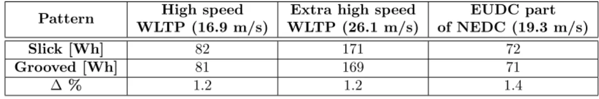
represents the difference between the grooved and the slick. . . 36 1.5 Comparison of energy consumption between slick and grooved tyre, calculated

with two different tests. . . 37 3.1 Comparison between the main geometrical features of wheels A and B. . . 52 3.2 Overall dimensions of the refinement boxes, with their shape and their level specified. 56 3.3 Summarizing table of the meshes and their results. . . 58 3.4 Integral quantities results for the three turbulence models with y+ below one. . . 64 3.5 Integral quantities results for the three turbulence models with high y+ respect

to the reference one. . . 67 3.6 Schematic view of the combination tested in this work regarding the steady state

simulations. . . 72 3.7 Schematic view of the combination tested in this work regarding the unsteady

simulations. . . 72 4.1 Table for comparison of the ventilation moment coefficient value in wheel A, for

the rotating models presented in tables 3.6 and 3.7. . . 91 4.2 Table for comparison of the drag coefficient value in wheel A, for the rotating

models presented in tables 3.6 and 3.7. . . 92 4.3 Table for comparison of the lift coefficient value in wheel A, for the rotating models

presented in tables 3.6 and 3.7. . . 92 4.4 Table for comparison of the ventilation moment coefficient value in wheel B, for

the rotating models presented in tables 3.6 and 3.7. . . 93 4.5 Table for comparison of the drag coefficient value in wheel B, for the rotating

models presented in tables 3.6 and 3.7. . . 93 4.6 Table for comparison of the lift coefficient value in wheel B, for the rotating models

presented in tables 3.6 and 3.7. . . 94 4.7 Table for comparison of the difference in the ventilation moment coefficient value

between the patterns, for the rotating models presented in tables 3.6 and 3.7. . . 95 4.8 Table for comparison of the difference in the drag coefficient value between the

4.9 Table for comparison of the difference in the lift coefficient value between the patterns, for the rotating models presented in tables 3.7 and 3.6. . . 96 4.10 Schematic comparison of the computational cost and of the runtime used by the

Sommario

Nel moderno mondo automobilistico l’efficienza energetica, sempre pi`u ricercata anche a seguito della diffusione dei veicoli elettrici, `e divenuta uno dei focus principali. Ridurre la resistenza aerodinamica `e sicuramente una delle possibilit´a pi`u interessanti per migliorare le prestazioni e ridurre i consumi. In particolare, l’interazione tra ruote e carrozzeria influenza sia il flusso esterno, che quello inferiore al corpo vettura. Per questi motivi, i produttori di pneumatici quali Pirelli Tyre S.p.a. stanno sviluppando battistrada ad alta efficienza, anche aerodinamica, agendo su parametri geometrici quali la spalla dello pneumatico e le scanalature. Da qui sorge l’esigenza di analizzare e comprendere l’interazione tra il flusso dell’aria e differenti battistrada, ed altrettanto importante diventa la sua modellazione nel caso di un’analisi CFD. Diversi studi sono gi`a stati condotti a riguardo, sia sperimentali che numerici, ma vista la complessit`a del flusso nel caso di uno pneumatico completo, non tutti i risultati sono concordi tra loro. Questa tesi analizza in maniera approfondita, tramite CFD, diversi modelli di calcolo, testando due differenti tipi di battistrada creati appositamente per questo studio. Le simulazioni svolte prevedono la ruota posta in rotazione e sollevata da terra, per rendere possibile l’utilizzo della Sliding Mesh (SM), ritenuto ad oggi il metodo pi`u fedele per riprodurre la rotazione di un oggetto. Le simulazioni svolte, stazionarie e non, sono quindi state paragonate all’approccio SM. Lo scopo di questo lavoro `e comprendere quale modello riesca a percepire meglio le differenze, in termini di coefficienti aerodinamici, tra i diversi battistrada considerando anche il fattore chiave di costo computazionale. Le equazioni impiegate per l’analisi sono le RANS, estremamente diffuse nelle simulazioni a scopo industriale, ed il software utilizzato `e OpenFOAM V6. Dai risultati emerge come le simulazioni stazionarie siano molto meno dispendiose dal punto di vista computazionale rispetto a quelle instazionarie e come il modello Moving Reference Frame (MRF) stazionario riesca ad ottenere buoni risultati con il minor costo possibile.

Abstract

The term ”energetic efficiency” has become one of the most important in the automotive world, especially with the spread of electric vehicles. For this reason, one of the possible direction of improvement is the reduction of the aerodynamic drag. Speaking of the underbody of a ground vehicle, it has a huge influence on the drag and the interactions between the wheels and the car body influence both the external flux and the under flow of a car. Hence, tyre manufacturer like Pirelli Tyre S.p.a. are developing high efficiency tyre pattern, by working on the geometric parameters like the shoulder radius or number and position of the grooves. In this context, understanding the interactions between different patterns and the flow is of primary importance, as the modelling in the case of a CFD analysis. Several studies have been already conducted, both in wind tunnels and using Computational Fluid Dynamics software. However, due to the complexity of the flow field around a rotating wheel, the results are not always in accordance to each other. Hence, in this work several approaches were tested on two different tyre patterns, created on purpose for this analysis, both in steady and unsteady conditions, in order to understand which is able to best combine precision and computational effort. The wheels were tested in a free stream flux, while rotating in mid–air to avoid any kind of complications due to the contact patch. Moreover, in this way the Sliding Mesh approach was exploitable, and it was taken as a reference result to compare the other methods. The equation adopted were the RANS, since they are the most used by the industrial world regarding the CFD analysis. To execute the whole simulation, starting from the mesh creation until the calculation of the equations, the software used was OpenFOAM V6. The results highlight that the computational cost of the steady simulations is much lower respect to the unsteady ones, while the SM approach doubles the hours used for the latter. Moreover, the steady Moving Reference Frame (MRF) approach is able to obtain good results with the lowest computational cost.

Breve estratto in lingua italiana

Questo lavoro `e nato a seguito della richiesta di Pirelli Tyre S.p.a. di studiare i possibili miglio-ramenti dal punto di vista aerodinamico di una ruota stradale, agendo su parametri geometrici fondamentali quali il numero e la dimensione delle scanalature, dei traversini e sulla forma della spalla dello pneumatico. Per poter eseguire lo studio, prima di tutto, si `e reso necessario capire come tutte queste componenti potessero essere modellate all’interno di una simulazione CFD. Diversi precedenti studi, sia sperimentali che numerici, sono stati svolti sull’aerodinamica di una ruota in contatto con il terreno. La maggior parte per`o tratta di pneumatici slick o, al pi`u, con le sole scanalature longitudinali, senza inserire i traversini laterali nel modello. Lo scopo di questa tesi `e quindi individuare un approccio che simuli, il pi`u fedelmente possibile, la rotazione di una ruota stradale completa e la sua interazione con il flusso esterno. Allo stesso tempo per`o, occorre limitare al minimo il costo computazionale: questo tipo di simulazioni infatti dovrebbero essere facilmente utilizzabili da Pirelli Tyre S.p.a. per comprendere gli effetti di una modifica al battistrada a scopo aerodinamico.

Il software utilizzato per eseguire le simulazioni, dalla preparazione della griglia al calcolo vero e proprio, `e OpenFOAM V6. Per centrare gli obiettivi preposti, si sono utilizzate le equazioni di Navier–Stokes mediate (RANS) nella loro forma stazionaria ed instazionaria. Inoltre sono state applicate le ipotesi di flusso isotermico ed incomprimibile, per semplificare ulteriormente le equazioni. Al fine di comprendere quale approccio fosse in grado di carpire le differenze tra i vari tipi di battistrada, sono state modellate due ruote complete di scanalature e traversini tramite il software Cati`a V5. Il cerchione `e stato sostituito da una semplice parete su entrambi i lati, in modo da ottenere una faccia perfettamente piana sul lato dello pneumatico. In questo modo l’analisi risulta completamente indipendente dal tipo di cerchione utilizzato. Le differenze tra i battistrada risiedono nella diversa configurazione di scanalature e traversini e nel differente raggio utillizzato per approssimare la forma delle spalle. Inoltre, le ruote sono state suddivise in tre aree, identificabili in lati, battistrada e spalle: ci`o ha reso possibile l’identificazione dei singoli coefficienti aerodinamici per ognuna di queste zone, per tutte le simulazioni.

Per la miglior fedelt`a dei risultati `e stata data molta importanza alla qualit`a della griglia di calcolo. In particolare, dopo una serie di test, `e stata rilevata l’importanza che le celle in corrispondenza della ruota ne assumano la forma stessa, in modo da approssimare fin da subito l’oggetto trattato. Inoltre, il bloccaggio `e stato mantenuto al di sotto dell’1% e la lunghezza della galleria `e stata tenuta pari a 30 diametri dello pneumatico. In ultimo, per ottenere una buona approssimazione del profilo di velocit`a a parete e quindi anche degli sforzi viscosi, sono state utilizzate 10 celle di layer il cui minimo spessore a parete `e di 1 ∗ 10−5_{m. Questo ha permesso di}

ottenere valori di y+ minori di 5 sulla maggior parte della ruota. Dopodich`e, `e stato effettuato uno studio di convergenza della griglia, il cui risultato porta ad ottenere 12 milioni di celle. Dato l’enorme costo computazionale che questa avrebbe comportato per eseguire le simulazioni instazionarie (costo incompatibile con le reali necessit`a di Pirelli Tyre S.p.a., a cui questo studio `e rivolto), la griglia di calcolo usata per le simulazioni instazionarie `e stata alleggerita fino ad

ottenere circa 3 milioni di celle. Inoltre, per evitare complicazioni e per poter utilizzare la Sliding Mesh (SM), la ruota `e stata simulata sospesa a mezz’aria in modo che non ci fossero interazioni con il terreno. Quest’approccio `e ad oggi generalmente riconosciuto in ambito tecnico come il miglior metodo per la modellazione di oggetti in rotazione, ed `e quindi stato considerato come punto di riferimento tra le simulazioni.

La velocit`a del flusso `e stata impostata a 12.5 m/s, che si traduce in un numero di Reynolds basato sul diametro pari a 5 ∗ 105_{. La velocit`a tangenziale della ruota `e equivalente a quella}

asintotica dell’aria, mentre la direzione di rotazione `e tale da creare una forza deportante per via dell’effetto Magnus. L’intensit`a di turbolenza all’ingresso del tunnel `e stata impostata a 0.2%, visto che si tratta di un problema di aerodinamica esterna.

Un attento lavoro `e stato svolto anche per quanto riguarda la scelta del modello di turbolenza. Sono quindi state eseguite delle ulteriori simulazioni 2D di una geometria simile ad un dosso stradale posizionato al centro della galleria virtuale, utilizzando quattro differenti modelli di turbolenza: il realizable k–ε, il RNG k–ε, lo Spalart–Allmaras ed infine il k–ω SST. Per la scelta, sono stati considerati diversi parametri analizzati, tra cui il numero dei layers, i valori di y+ raggiunti, i coefficienti aerodinamici e gli sforzi viscosi. Ne `e risultato che il k–ω SST sia il modello pi`u adatto per questo tipo di applicazioni, a patto di mantenere il valore di y+ al di sotto di 60.

La velocit`a di rotazione tangenziale degli pneumatici `e stata sempre modellata tramite la condizione al contorno data da rotatingWallVelocity (RWV). Per la modellazione dei traversini invece sono stati utilizzati tre diversi approcci, comuni tra le simulazioni stazionarie e non:

1. Moving Reference Frame (MRF);

2. `e stata applicata una velocit`a normale alle facce del traversino, per simulare il movimento dell’aria al loro interno;

3. non `e stata applicata alcuna condizione aggiuntiva, fatto salvo per la RWV.

Un altro metodo consisteva nell’applicazione del MRF sia all’interno dei traversini, che nelle scanalature. Si `e rivelato per`o scorretto, dato che la soluzione risultante ha mostrato una netta riduzione della velocit`a dell’aria al di sotto della ruota, fenomeno incompatibile con la realt`a fisica del fenomeno.

Le simulazioni stazionarie non sono riuscite a raggiungere la convergenza dettata dalle toller-anze dei residui, impostate a 1 ∗ 10−3 _{per la pressione ed a 1 ∗ 10}−4 _{per la velocit`a e le quantit`a}

turbolente, a causa dell’intrinseca instazionariet`a del problema in esame. In ogni caso, una volta che i residui hanno raggiunto il loro minimo e che i coefficienti si sono stabilizzati, sono state estratte le quantit`a di interesse tramite un’operazione di media tra le ultime 500 iterazioni. An-che per le simulazioni instazionarie, una volta An-che il dominio di calcolo `e stato completamente investito una volta dal flusso d’aria, `e stata eseguita una media su 0.16 s, corrispondente al tempo necessario alla ruota per compiere una rotazione. Questo lasso di tempo corrisponde al periodo delle fluttuazioni dei coefficienti, pertanto si `e ritenuto sufficiente per svolgere l’operazione di media. Questa non `e stata per`o possibile col metodo Sliding Mesh a causa della rotazione della griglia di calcolo secondaria, che porta le celle al suo interno ad avere i campi mediati non solo rispetto al tempo, ma anche alla loro posizione e quindi non utilizzabili allo scopo.

In conclusione, dall’analisi dei risultati, emerge che sia le simulazioni stazionarie che le in-stazionarie sono in grado di riprodurre in modo corretto le caratteristiche principali della scia di riferimento. Tuttavia, alcuni elementi caratteristici come vortici e regioni di bassa velocit`a sono rimasti esclusivo appannaggio della Sliding Mesh. Per quanto riguarda la differenza dei coeffici-enti aerodinamici tra i due tipi di battistrada, rispetto ai risultati della Sliding Mesh, il metodo

MRF stazionario ed il secondo approccio instazionario, con l’aria in movimento all’interno del traversino, hanno ottenuto il miglior riscontro.

Dal punto di vista del costo computazionale, di fondamentale importanza nello studio richiesto, le simulazioni stazionarie risultano nettamente in vantaggio rispetto alla controparte instazionaria, nonostante l’enorme differenza tra le griglie utilizzate. Inoltre, la preparazione del secondo ap-proccio `e certamente pi`u laboriosa rispetto ad un pi`u semplice MRF. Per questi motivi al ter-mine degli studi effettuati, risulta che il Moving Reference Frame, associato ad una simulazione stazionaria, sia il miglior metodo da utilizzare per la modellazione di ruote complete e per com-prendere le differenze tra diversi battistrada.

Introduction

Nowadays, the world attention about the environmental theme is growing exponentially and every single energetic aspect is analysed and improved in term of energetic efficiency. Especially the automotive manufacturers are involved in this green wave and the customers themselves are beginning to take care of the environmental impact of cars and fuel consumption. In a few words, customer needs and energetic efficiency are the key words in this field. The rising of the electric vehicle, becoming in these years more and more popular and economically accessible to the middle class, can be a good example of the effort in this direction. From this point of view, aerodynamic drag for ground vehicles is of primary importance because it impacts on power consumption of a petrol or electric car by 75% [5] and this suggests that one of the possible direction of further automotive technology improvement is the drag reduction, that will also help to extend the autonomy range of an electric vehicle.

Scientifically, the drag force is defined as the force that acts against the relative movement between an object and a fluid and can be decomposed in two different contributes: skin friction and base drag. The first one is only due to the interaction between the fluid and the object where, due to its viscosity, the fluid tends to adopt its velocity to that of the object and vice versa. The second one is due to the pressure distribution that arise around the surface of the object according to Navier–Stokes equations: the difference between forward and backward pressure, integrated along the surface, leads to a drag force.

Regarding the aerodynamic bodies, they can be divided into two specific classes which are characterized by different shapes, different flow field around them and different drag contribution: bluff bodies are characterized by massive flow separation. They don’t have a preference di-rection of stretch, instead the ratio between dimensions remains close to one. Their main source of drag is the base drag, since the detached flow has little impact on the skin friction while forms huge recirculations bubbles with a lower pressure respect to the asymptotic value. The typical example of a bluff body is the cylinder and every kind of road vehicle fall in this category;

streamlined bodies are featured by attached flow along the major part of the body. Usually they have a preference direction of stretch and are characterized by smooth, rounded and streamlined surfaces. A typical example is the airfoil shape. In this case the main drag contribution is given by the skin friction, and usually their drag coefficient is much less respect to the first class.

Many efforts have been made during the years by the designers to reduce the drag force on bluff bodies class, sometimes with strange body shape adopted. However, car body aerodynam-ics improves a lot thanks to more rounded shapes or particular design technique like the Kamm tail. Nowadays, the aerodynamics efficiency of road vehicles seems that have reached a limit regarding the external body shape optimization. Furthermore, the designers must consider also

the customer tastes (that are often very far from an aerodynamic body, with sharp edges and wide shapes) and safety parameters. As examples, lowering the vehicle height from the ground or placing an engine undercover meets all the requirements, while an air deflector placed upstream of the wheel has not being implemented in modern road cars, even if are known its aerodynamic advantages [19]. Despite these minor efforts, even less has been made to improve the aerody-namics of the underflow and of the wheels of a car, which are strongly coupled and impacts also on the overall car wake. As proof up to 30% of the car aerodynamic drag comes from wheels [5] [6] [14] [26], and a combined effort between cars manufacturer and tyres makers could surely reduce this percentage. In a modern Formula 1 car this contribution is even more important and their effort to guide the flow above or aside the wheels can be seen in the recent prototypes, where their front wing can produce upwash or sidewash to avoid the direct impact of the flow field on the wheels. From an aesthetic and functional point of view, a correct design of wheel covers shape and a flow study of them can reduce the amount of mug and dirt deposition on the vehicle body and this is an important aspect from the customer point of view.

Pirelli Tyre S.p.a., leading tyres producer, with the collaboration of Politecnico di Milano, is studing and developing low drag and low friction tyres. The common objective is to develop and to test different kind of tyre patterns that can guarantee excellent mechanical performances in terms of handling and water drainage and also improvements in terms of aerodynamic drag: the position, the number and the orientation of the grooves could play an important role; the shoulder shape and the tyre deformation due to the weight crush are surely crucial factor.

Several investigations, both experimental and numerical, have been made to characterize the flow field around a wheel. They include tyres in contact with the ground, rotating in mid–air, inside a wheel cover or with full vehicle test. However, the experimental results are not easy to be obtained since the facility that allows the crush of the wheel in order to obtain its correct deformation and its rotation are few. Moreover, obtaining data in these condition is not easy at all and very often only integral quantities (forces and their coefficients) and pressure distribution along the circumference can be obtained, while the flow field in the wake can be reconstructed by placing a grid of probes behind the wheel. These aspects obviously pushed the effort of the research to the Computational Fluid Dynamic (CFD). However, also in numerical analysis there are a lot of complications, some of which will be discussed in this work and probably this is the reason why not all the analysis conducted in this field are in agreement regarding, for example, the numerical model that should be applied.

The focus of this thesis is to understand which numerical model is the most suitable and affordable for a massive CFD test campaign regarding the shape optimization of wheels pattern. To do so, several numerical simulations have been performed on an isolated wheel that can freely rotate in mid–air. Hence, the wheel won’t be deformed by the weight and won’t produces any contact patch. This set up, that can seems incoherent with the case under study, is necessary for the application of a particular numerical model called Sliding Mesh, described in section 2.6, that is the most powerful and reliable tool to study rotating objects. Moreover, this simplified set up could guarantee fewer meshing problems and hence more robustness of the results.

An important note to avoid misunderstandings regards the definition of the reference frame used in this work. The figure 1 should help in the comprehension. The centre of the wheel corresponds to the origin of the frame of reference. The air flow points towards the positive X direction, while the Z axis defines the positive direction of the lift. The third axis Y, according to the right–hand rule, defines the surface normal direction of the side of the wheel. Therefore, its angular position θ and its angular velocity ω are defined positive in the opposite direction respect to the Y axis, and the angle θ starts from the forward stagnation point of a stationary cylinder. Unless otherwise noted, this frame of reference is valid for all the presented thesis.

Figure 1: Graphical representation of the reference frame adopted in this work.

• Cati`a V5 for the design of the required geometry and their exportation in step file; • Salome for the conversion of the step file into a high quality stl file;

• OpenFOAM 6 for the entire analysis process, which include mesh generation, the simulation itself and part of results extraction;

• Paraview for the visualization and the extraction of the results; • Matlab and Excel for further data extraction.

The choice fell on these software because three of them (Salome, OpenFOAM and Paraview) are opensource and this allows the author to get the access to the complete version of the program. Moreover, in that way every simulation is easily reproducible. Cati`a V5 and Matlab are provided by the university Politecnico di Milano, but the first one can be easily substituted with another cad software, while the second one has its opensource counterpart.

Chapter 1

State of art

In this chapter is presented a short review of what are the experimental and numerical works that have been conducted on rotating wheels until now. First, a brief explanation of the wind tunnel tests and of the physical phenomena that involve wheels aerodynamics is presented in section 1.2, secondly is presented an overview about the CFD variables and results in section 1.3. More attention is put on the numerical simulation, since it’s exactly what this work would investigate.

In the last section 1.4, are presented the critical aspects of the numerical simulations con-ducted thus far.

1.1

The simplest case: 2D cylinder

The simplest, yet direct connection to deal with a wheel is reduce its analysis to a 2D cylinder instead. A lot of different studies were conducted on cylinders, with various boundary condition and within a wide range of Reynolds numbers. What is known is that a non rotating cylinder immersed in a flow field behaves like a bluff body, even if its surface is perfectly smooth: this is expected since it hasn’t a streamlined shape. Its wake structure strongly depends on the Reynolds number at which the experiment is performed. The Reynolds number is defined as Re=ρ U D_µ , where ρ is the fluid density, U is the freestream magnitude velocity of the flow, D is the characteristic length (which is the diamenter when dealing with a cylinder or a wheel) and µ is the dynamic viscosity. No lift force is produced in this case, exept for a particular flow regime in which the so called Von Karman vortices detaches from the cylinder; in that case, both lift and drag show oscillating behaviour. However, the medium value of lift in time remains zero. Dealing with a rotating cylinder, the Reynolds number is not the only parameter that count, since also the direction and velocity of the rotation matters: the flow field that established behind a rotating cylinder deflects respect to a non rotating one and both the direction and the magnitude of this deflection depend on the sense of rotation and its speed. Along with a path deviation of the flow, a rotating cylinder experiences also a lift force which is directly proportional to the angular velocity, due to an asymmetric distribution of the flow field. This effect is also known as Magnus effect and it is observed also in potential flows, which formally have no viscosity, through an artificial addition of the circulation. For example, a counter clockwise rotating cylinder immersed in a flow that travels from left to right produces downforce. When the cylinder is put in contact with a surface only from one side, for example when it rotates on the ground, the Magnus effect can’t work anymore since the air is forced to pass on the top side

of the cylinder: this effect creates a positive lift, in opposite to what is stated by the Magnus effect. A representation of the situations just described is visible in figure 1.1.

Figure 1.1: Stream lines and pressure distribution along a cylinder [27]: A:stationary, free stream; B:rotating, free stream;

C: stationary, in contact with the ground; D:rotating, in contact with the ground.

These behaviours can be expected also for an isolated wheel that can freely rotates in mid–air or on the ground.

1.2

Wind tunnel tests

A wheel, like the cylinder, is a bluff body that produces high drag and a wide separated region, with turbulent wake structures. Several authors focus the attention on the aerodynamic of the wheels using wind tunnel experiments.

One of the first resercher was Morelli [22] which, in 1969, tested a Formula 1 racing wheel under rotating condition in a wind tunnel. He measured lift, drag and aerodynamic moment and he found that a faired rim reduced the drag force by 22% and that the drag doubled when the wheel was tested with a yaw angle of 20◦ _{respect to a zero yaw angle condition. However, the}

tyre was lifted from the soil and produces downforce due to the Magnus effect, so the impact of the contact patch was not taken into account.

Also Stapleford and Carr [30] analyzed a wheel in free air in stationary condition. They set the Reynolds number according to the typical operating velocity of a ground vehicle. In these conditions the flow has a symmetrical distribution of velocities and pressures around the wheel, both along the longitudinal and the transversal planes. It remains attached for 120◦ _{from the}

forward stagnation point, considered the zero angle. At the forward stagnation point the value of the pressure coefficient CP is obviously one and it decreases until it reaches the minimum value

at 90◦_{where, for the Bernoulli theorem, can be found the maximum velocity of the flow. The C} P

then rises again until the separation point; after that it remains constant in the backward of the wheel. As for the cylinder, no overall lift is produced. They were the first to discover that a wheel in contact with the ground produces lift, regardless if it’s rotating or not and this highlights an opposite behaviour respect to what is suggested by Magnus effect. Moreover, they noted that the wake extends widely and further respect to the lifted wheel case, increasing the drag coefficient. Also, the rotating wheel shows lower CD and higher CPall along the topside respect to the one

observed in stationary condition, even if both are in contact with the ground: this translates in a lower lift force and lower drag for the rotating one. As soon as a ground clearance appear, the air flux could evacuate under the wheel and the positive lift measure disappears.

Cogotti [26] [27] performed a series of experiments where he gradually reduced the clearance between the wheel and the ground. The pressure below the wheel keeps reducing until the wheel touches the soil. In this way he demonstrated that a tyre produces lift as soon as it’s in contact with a wall. He also supposed that an isolated wheel produces three pairs of vortices, clearly visible in figure 1.2: two horseshoe vortices caused by the contact patch between the wheel and the ground (numbers one and two), two shoulder vortices caused by the upper point of separation (numbers three and four) and two vortices placed in the middle of the tyre (numbers five and six). However, this is an assumption based only on theoretical point of view and no observation were made.

Figure 1.2: Main vortical structures produced by a wheel in contact with the ground [21].

Moreover, he confirmed the huge differences between a stationary and a rotating wheel, even if both are in contact with the ground, since lift and drag are 40% and 25% lower in the second case and the rotation of the wheel moves the forward stagnation point 15◦ _{down respect to the}

stationary one.

As regard more specifically rotating wheels experiments, Fackrell [8] was one of the first who conducted a deep and complete analysis about this topic and his conclusions are still taken into account as reference results. The facility where he took the tests was up to date: it was equipped with a conveyor belt to simulate the moving floor, with a roller to allow the rotation of the wheel and with an air suction system just before the belt to minimize the boundary layer influence. He used three tyres width and two shoulder profiles, for a total of six wheels. The Reynolds number used in his experiment was 5.3 ∗ 105 _{and he was able to measure the static pressure}

along the circumference of the wheel thanks to 25 probes. The aerodynamic forces and their coefficients were calculated through the integration of the static pressure along the surface. He tested both stationary and rotating wheels and he confirmed what Stapleford and Carr [30] found

during their tests. In figure 1.3 is shown the pressure distribution of a rotating and a stationary experiment along the centreline of one of the wheels.

Figure 1.3: Values of the pressure coefficient along the centreline of the wheel [8].

He discovered that the separation point is located approximately at 270◦ _{and he supposed}

that the conditions that allow the detachment were zero velocity U and zero ∂U

∂t. A pressure

peak right in front of the contact patch was found, with a value of pressure coefficient up to two; it can be explained through the fact that both the belt movement and the tyre rotation provide energy to the flux, which converges right at the junction with the ground. This encourage the so called ”jetting effect” especially in a slick tyre, where the air is completely blocked between the wheel and the ground. The effect was already observed by Morelli and consists in the formation of two counter rotating vortices in the lower part of the wheel (numbers one and two in figure 1.2) due to the high pressure gradient respect to the outer region. This phenomenom is also present in a stationary wheel in contact with the ground but, according to Fackrell, the rotation increased significantly this behaviour. Furthermore, it leads to a premature detachment of the boundary layer by changing the location of the stagnation point on the top of the wheel, hence he supposed some sort of correlation between the jetting effect and the flow detachment.

Comparing a narrower wheel with more rounded profile respect to the previous one, he noticed that the pressure on the top and behind the second wheel is more negative, hence he concluded that the edges profiles have a certain influence that is measurable even along the centreline. Moreover it has lower CD but higher CL respect to the first one.

Mears [21] tested different tyres pattern such as slick and grooved. He found out very diffferent pressure distributions at the contact patch. In the grooved tyre the air could flows through the grooves from the high pressure zone created at the contact patch to the backside of the wheel. This leads to a huge pressure drop due to the Venturi effect inside the grooves and diminishing the size of the vortices. On the other side, a slick tyre suffers of a massive jetting effect caused by the squash of the air between the rotating tyre and the ground. Due to this phenomenom, he prooved that there is a difference in aerodynamic drag between a slick and a grooved tyre. Immediatly

after the contact patch, experimental results conducted by Mears [21] shows a sudden pressure drop: this effect was called ”suction cup” effect and consists in a vacuum creation between the tyre and the ground, which vanishes once that the tyre lifts up, leading to a pressure recovery.

1.3

CFD simulations

Nowadays, the trend is to use Computational Fluid Dynamics (CFD) to analyze a lot of different cases without the cost and the effort that a massive wind tunnel test campaign would require. A virtual reproduction of the wind tunnel is usually recommended to calibrate the computational model. The only drawback of this approach is the intrusivness of the instruments and the disturbances that the supports can cause to the flow, since both aspects are completely absent in simulations and can falsify the comparison. After that, the attention can be focused on the flow behaviour, since CFD analysis allow a complete visualization of the aerodynamic fields. In fact, the post processing phase of a simulation is much easier respect to take the measurements of interest in a wind tunnel test. During the last twenty years the use of Computational Fluid Dynamics has become more and more affordable also for complex cases thanks to the exponential growth of computer power. Despite this huge technology push, discretize and solve the full set of Navier–Stokes equations for external aerodynamics remains a very tough and expensive work, hence simplifications to the model are always applied. For example unsteady studies remains often out of the question for the major part of the industrial world due to high requirements in computational power, even if the flow around a rotating wheel, which is a bluff body, is without any doubt 3D and unsteady. A common simplifications adopted by every study performed in this topic are the hypothesis of isothermal and incompressible flow, since there are no heat sources and the Mach number (defined in section 2.1) is largely lower than 0,3. These hypothesis allow to reduce the computational effort.

However, the biggest problem and the most time–consuming part of every CFD analysis remains the so called pre processing phase, that groups all the preliminary activities before the calculation. The aerodynamic analysis of a wheel it’s not an exception: in particular, the main issues encountered are the choice of the rotating model presented in section 2.6 and the meshing criteria in section 3.2. For example, the contact patch area gives very often big trouble because the wheel is almost tangent to the ground; or the rim angular position, especially if it has few spokes, could influence the results of the simulation. In this section are also presented some solutions found by previous analysts to these sort of problems.

The simulations conducted thus far include tyre with different patterns, with and without longitudinal and lateral grooves, different shoulders shapes and spokes positions. Varius strategy were developed in order to obtain a correct mesh generation and different turbulent models were tested both in unsteady and steady simulations. In order to understand the solidity and relia-bility of the model, one can compare the results of the CFD with the wind tunnel experiments. However, it must be sad that even a wind tunnel test is not free from mistakes: the instruments always suffer of noise and measurement errors and different tunnels provide several dimensions and turbulence intensity. For example, Fackrell’s experimental campaign [8] has been conducted in the 70s, hence a reply of its tests with modern instrument and tunnel could lead to better and more reliable results.

1.3.1

Rotating model approach

The correct choice of the rotation model has two main objectives: • to simulate a wheel rotation with the highest possible fidelity;

• to avoid meshing problems and wasting of computational power by using the best approach, depending on the situation.

For example, SM is the highest fidelity method to account for rotating surfaces, but it requires unsteady simulations and hence huge computational effort.

Hobeika and Sebben [14] performed some simulations on two isolated, symmetric wheels with open rim, both rotating in free stream at 100 km/h. The asymptotic velocity of the flux was set at 1 km/h, in order to avoid any kind of influence on the field around the wheel. They used a slick and a grooved pattern with the same dimensions and profile. The grooved one was a fully detailed tyre, with both central and lateral grooves. The lateral grooves were 5 mm wide, 5 mm deep and they extend for 40 mm toward the centre of the tyre; the longitudinal (or rain) grooves were four, their width was 10 mm and their depth 6 mm. As explained in section 2.6, every rotating model can simulate the rotation in a different way, and can be suitable for a specific case. By adopting such different tyre pattern, the authors could guarantee that the best method was used for every kind of wheel. They adopted the same mesh settings between simulations. The tunnel had a length of 20 m, a width of 8 m and an height of 10 m. The y+ values achieved were below one in the majority of the wheel. This results was possible thanks to 8 layers with an expantion ratio of 2.0, starting from a maximum surface cell size of 2 mm and with the first layer thickness of 0.01 mm. The overall number of cells was about 10 million. In this case the simulations were performed with the rotating tyre in mid–air, hence the wheel shape is not influenced by the side bulge or by the contact patch. The circular perfect shape allowed the use of the SM approach.

They divided the wheels in three main regions: 1. the complete tyre;

2. the rim spokes; 3. the lateral grooves.

They chose the ventilation moment (that is the torque that acts against the wheel rotation) splitted between the regions to compare different combinations and to understand the capabilities and the failings of every rotating model. As reference, zero rotating velocity corresponds to null ventilation moment. The SM approach is considered the reference one: closer results to it translates in a good reliability of the simulation.

For the slick tyre they made four tests: S1: SM on both regions one and two;

S2: SM on region two and RWV on region one; S3: RWV on both regions one and two;

S4: SM on region one and RWV on region two.

From figure 1.4, it can be seen that the best method is the second one: both the total ventilation moment and the contributes of every single region are predicted extremely well, even if the tyre contribution is correct for all the methods. Apparently the use of the SM to simulate the spokes rotation is necessary, while the RWV is enough in case of surfaces that involves only tangential velocity. In this manner, Hobeika and Sebben [14] achieved optimal results with the lowest computational cost and the simplest model. Comparing also the velocity field, it is well represented along the tyre surface by all the methods. The correctness of both the velocity and the ventilation moment of the tyre are expected since the velocity along its surface is purely

tangential. Hence, the RWV method can be sufficient. On the other side, the velocity assumes very different values in the rim region, depending on the approach used: in fact, the air between the spokes doesn’t rotate at all in case only the RWV method is applied.

Figure 1.4: Ventilation moment for the slick pattern splitted between regions, for every combination adopted, found by Hobeika and Sebben [14].

For the grooved pattern they made five tests: G1: SM on all the regions;

G2: SM on region two and RWV on the rest; G3: RWV on all the regions;

G4: MRF in region three, RWV on the rest;

G5: RWV on region one, SM on region two and MRF on region three.

In this case the best combination was the last one: both the total ventilation moment and the contribution of the single region are almost the same as the fully SM method. The results are presented in figure 1.5. As for the slick tyre, Hobeika and Sebben [14] found that the contribution of the sole tyre is well predicted by every combination; the difference is made by the rim, that confirms the need for the SM and by the grooves, which require at least the MRF approach. The huge limitation of the RWV method is the inability of introducing a normal velocity component respect to the surfaces involved. As regard the velocity field, the most evident discrepancy is its value inside the grooves and around them: while the full SM approach and the last combination are practically the same, the velocity magnitude inside the grooves modelled with the RWV is extremely low and doesn’t match at all the external velocity of the tyre. Furthermore, the tangential velocity just above the groove is not mantained since the high speed flow attached to the tyre must overcome the region of dead air before reaching the other side, losing part of its momentum. This phenomenom is completely absent in case of full SM or MRF and the

tangential velocity is maintained along the entire external surface. Looking into the pressure field, there are some local differencies between the full SM approach and the combination G5, especially in the third region, due to a limited interaction between the grooves and the outer flow when the MRF methos is applied.

Figure 1.5: Ventilation moments for the grooved pattern splitted between regions, for every combination adopted, found by Hobeika and Sebben [14].

Tyre Rim Grooves

S1 SM SM – S2 RWV SM – S3 RWV RWV – S4 SM RWV – G1 SM SM SM G2 RWV SM RWV G3 RWV RWV RWV G4 RWV RWV MRF G5 RWV SM MRF

Table 1.1: Summarizing table of the possibilities.

Hobeika and Sebben [14], based on the results of every analysed combination summarized in table 1.1, finally proposed this hybrid approach in order to take advantage of the best features of every rotating models:

• RWV can be used along the external tyre area, where the velocities are only tangential to the surfaces;

• MRF region is builded only inside the lateral grooves, which are smalls and extremely repetitive (hence the solution should not be influneced by their position);

• SM is adopted in case the wheel setup includes an open rim with rotating spokes.

The authors tested different combination of rotating models in order to compare the results and understand which one should be used, considering the geometry and the computational power.

Their conclusion is that to deal with a slick tyre is necessary the application of the SM approach only in the rim region, where the air must have a normal velocity respect to the spokes. They understand that the MRF approach doesn’t predict well the rim region because the solution was location dependent respect to the few spokes present. The RWV approach can be used along the tyre surface. For the grooved tyre, the consideration made for the previous pattern are still valid, but the new region required at least the MRF approach in order to be correctly modelled. These mixed approaches lead the two analyst to a good prediction of the ventilation moment and of the velocity field, while they were able to mantain the lowest computational cost possible. However, they noted that even if both the overall and the partials ventilation moments are well predicted as already highlighted, the contribution between shear and pressure contribution for the grooved tyre remains quite far from the reference case G1.

The analysis conducted by Hobeika and Sebben [14] among different rotating methods for two different types of tyre pattern are useful to understand the problems related to modelling different parts of the same wheel and help in the comprehension of the ventilation moment contribution. Unfortunately, an important test that was not conducted is the application of the MRF in the rim region in substitution of the Sliding Mesh. This approach, to the author’s opinion and knowledge, should give similar results respect to the Sliding Mesh especially in case of frequent spokes in order to not have any dependencies from their position and removes part of the computational effort.

1.3.2

Shoulder type and hub influences

To understand the influence of the shoulder geometry and of the hub Diasinos, Barber and Doig [7] took as a baseline tyre the ”A2” used by Fackrell [8] in his experiments and replaced the original shoulder shape with a constant radius. Moreover, they cover the wheel hub to obtain a closed rim design, easier to deal with. The baseline wheel of Fackrell [8] had a width of 191 mm and a radius of 208 mm; the modified tyre had the same dimensions, while the radius of the shoulder was 24 mm. The simulations were conducted on a rotating wheel leaning on the ground and the contact patch was modelled with a step whose height was 0.0028 of the wheel diameter. This operation was done to avoid mesh problems in that region. The mesh adopted allowed the y+ value to remains below one in the regions of attached flow and a grid convergence study was conducted, leading the final mesh to had approximately 8 million cells. The turbulent model tested were the realizable k–ε and the k–ω SST, yielding very similar plots when comparing the CP value along the wheel circumference. They focused their attention on

a steady state simulation performed with RANS solution. To validate the results of the steady state simulations they also ran some transient simulations, described in subsection 1.3.4.

Regarding the results, they immediately observed two additional vortical structures, smaller than the others, only on the baseline wheel. Their explanation to this phenomenon is that the vortices, visible in figure 1.6, were formed by the shear interaction between the flux and the flat sides, while the other were formed by pressure variations. The evidence found by Diasinos et al. [7] is in contrast with Fackrell’s observation: he found no proofs of these additional vortices in wind tunnel experiment. Nevertheless he used a wheel with the hub, hence there was no shear interaction between the flow and the side of the wheel since the latter was not flat. The

wheel with the covered hub experienced a huge reduction both in drag and lift and this obviously reflects on their coefficient, as shown in table 1.2. Also, as could be expected by looking at the coefficients, the no–hub wheel had a narrower wake, even if it was higher.

Figure 1.6: Flow structures for the A2 rotating wheel [7]; a: with hub, x/d=0.64; b: without hub, x/d=0.64; c: with hub, x/d=0.75; d: without hub, x/d=0.75.

Regarding the constant radius shoulder case, Diasinos et al. [7] observed a region with higher static pressure, probably responsible of the drag increase. Moreover, a wider and lower wheel wake was observed since the constant radius slightly augment the contact patch area: in this way the jetting effect formed the two characteristics vortices far from the centreline, probably changing also the position of the upper separation point. This delays the flow separation and leads to a rise of the 85% of lift generation. However, the basic flow structures between the two shoulder shapes are maintained.

Baseline Baseline, no hub Constant radius, no hub

CL 0.28 0.20 0.37

CD 0.51 0.47 0.51

Table 1.2: Comparison between wheels for the force coefficients.

Diasinos et al. [7] concluded that each simplification has its own weight on the flow field structure. For example, the hub closure and the constant radius approximation for the shoulder (which for sure can be considered a small geometric variations) alter the flux and the wake in different manners, but the changes in the integral quantities like forces and coefficients are of the same magnitude.

1.3.3

Stationary vs rotating

Diasinos et al. [7] focused their attention also on the differences between a stationary and a rotating isolated wheel since, from wind tunnel tests, their results were different. Two hypothesis were proposed to explain the huge discrepancies:

• the first one, proposed by Fackrell [8], stated a different behaviour of the primary wheel vortices. In particular, he supposed that the rotation of the wheel alters the path of the incoming flow by forming two vortices in front of the wheel. This should lead to a distorption in the wake and that would explain the differencies;

• the second one theorized that the reason laid in the boundary layer formation along the fixed soil in case of non rotating wheel, leading to a different jetting action.

However, further simulations performed by Diasinos et al. [7] didn’t confirmed these hypothesis. For the first one, the computational results contained no traces of vortices in front of the wheel. Diasinos et al. [7] investigated also the second one by replaced the stationary ground with a slip condition. In this way, a boundary layer can’t not born since the flow experiences no shear stress respect to the soil. Again, there were no differencies respect to a standard, non rotating wheel simulation, hence also the second hypothesis was discharged. Diasinos et al. [7] focused their attention on the comprehension of the location of the separation point, since it could be the primary reason of differencies both in the wake structures and of forces coefficients. They splitted the wheel geometry in two halves to investigate separetly the upper and the lower half rotation. The lower one included the angle between -45◦_{< θ <135}◦_{, the upper one the remained}

portion of the wheel. In the case where the lower half was rotating they employed also the moving ground condition, according to the tangential speed. In this way they were able to indipendently investigate the jetting phenomena, the location of the upper separation point and if some correlations between the two existed. They discovered that the jetting effect and the upper stagnation point are indipendent one from the other and the only thing that counted was which half was rotating. Hence, while the upper half was rotating, the separation point moved forward but no increment in the jetting effect was noted. Viceversa, even with the rotation of the lower half, the separation point was the same of a stationary wheel. The upper rotation also lead to the formation of the upper vortices, typical of a rotating wheel; however, in that case they were higher, proof that the jetting phenomenon has some influece on the location of the upper vortices.

1.3.4

Steady vs unsteady

It is well known that the flow field around a bluff body like a wheel is inherently unsteady. As sad, the problem is that the major part of the industrial world could not afford an unsteady simulations due to its cost.

For this reason, Diasinos et al. [7] looked for a steady, yet reliable solution. Using the overall set up described in subsection 1.3.2, they compared the behaviour on the same wheel of a steady simulation using Reynolds averaged Navier Stokes equations (RANS) with a transient one that used unsteady RANS (or URANS). They used two different time steps for the unsteady simu-lations, 0.5 and 0.25 millisecond respectively. The time step variation in a transient simulation modifies the convergence properties of the solution and affects the Courant number. The results between the two unsteady runs, averaged over 0.7 seconds, were almost identical. Hence, for further investigations, the 0.5 millisecond time step was adopted to speed up the simulation without loosing accuracy of the results.

The CP value along the wheel centreline was taken as comparative feature. In figure 1.7 the

results of both the simulations are shown. The unsteady simulation has been averaged over a period of 2.5 second. The differences lies in the separation point location, which is shifted of 2◦_{, and in the minimum value of the pressure reached right at the separation point, which has}

a lower absolute value in the steady simulation. Moreover, the authors explained the extremely regular oscillations of the force coefficients with the fact that the RANS approach is inherently diffusive, while in reality the flow behaviour woud be more chaotic.

Figure 1.7: Centreline CP distribution of Fackrell’s test, transient and steady RANS

They observed very little differencies between the steady state and the transient simulations, hence they confirmed the validity of the steady RANS approach and they developed the studies on this method, since the major effort to conduct a transient simulation, at least with URANS approach, was not worth it.

1.3.5

Step contact patch

The contact patch is a very tricky region to deal with. It’s the region where the tyre deformation takes place, so there is a crush of the wheel and a side bulge is formed. Moreover, the deformation is a characteristic feature different for every tyre and is affected by the dimensions, the side walls stiffness, tyre pressure, speed and vertical load applied. Finally, as already sad, the wheel is almost tangent to the ground: hence the mesh should guarantee very stretched cells to correctly follow the tyre profile. The problem is that these kind of cells can leads to high skew faces, that are one of the main problem in a simulation. This topic is better described in paragraph 3.2.

Diasinos et al. [7] investigated the aspect of contact patch simplification to understand how to reduce the meshing problems in that area and whether the results are affected by a change at the contact patch region. In particular, the authors extruded a dummy contact patch that sustains the rest of the wheel, just like a small pedestal. In that way, four small faces appear between the wheel and the ground. In particular, they used this technique:

1. the wheel was lowered below the ground as it should appear in real condition due to the ground crush;

2. it was cutted at the ground level in order to obtain a flat face;

3. it was raised above the ground by the amount of the ground crush used at point one; 4. a solid was extruded from the flat surface, creating a small pedestal.

More than one step height was tested in order to understand its influence on the simulations: the minimum was 0.0028 D, increased to a maximum of 0.0085 D, where D is the wheel diameter.

Increasing the step height translated in a higher height and a lower width of the wake, due to a change in the separation point location which moved backward. Since an increased step height also affects its aspect ratio (the ratio between its height and its width) the lateral speed induced by the jetting effect decreased. This is in agreeement with Fackrell [8] observation regarding the influence of the separation point respect to the jetting effect, since it is the major responsible for the two horseshoe vortices that depart from the contact patch. The relation between the step height, the jetting effect and the horseshoe vortices is clearly visible in figure 1.8.

Regarding the force coefficients, the higher is the step and hence the aspect ratio of the contact patch, the lower are the drag and the lift coefficients. The CD passed from 0.5 to 0.4, while the

CL was more sensitive, passing from 0.3 to 0.12. The difference in sensitivity is probably due to

the huge influence of the location of the upper separation point to the overall lift production. Diasinos et al. [7] concluded that the height of the contact patch is a fundamental parameter that must be considered as close as possible to the real case. This translates in the absence of dummy patches or, at leat, very small pedestal in simulations and in a correct vertical load when performing a wind tunnel test.

1.3.6

Slick vs grooved

Lesniewicz et al. [21] focus their attention on comparing two different tyre patterns, a slick and a grooved one. Their aim was to investigate the jetting effect phenomenon in both wheels and give an explanation to the drag difference between the patterns.

Figure 1.8: Total pressure contour plots along a normal plane at x/d=0.64 and on a plane parallel to the ground at z/d=0.015, for two different step height [7]:

a: step height=0.0028d; b: step height=0.0028d; c: step height=0.0085d; d: step height=0.0085d.

Both the tyres were based on the one used by Fackrell [8], with a diameter of 416 mm and a width of 191 mm, in order to compare the CFD simulations with the results obtained in a wind tunnel. The grooved pattern had only three longitudinal grooves, evenly spaced one from the other and symmetric respect to the wheel centreline. Their width is 6.35 mm and their depth is 3.18 mm. The contact patch was defined with a flat surface that leans on the ground, but the longitudinal grooves remain uninterrupted because their absence in the contact patch area would surely alters the results. Moreover, Lesniwicz et al. [21] removed the hub and closed the wheel with a flat sheet, as visible in figure 1.9. The resulting geometry is not symmetric due to the shifted position of the sheet respect to the centre.

Figure 1.9: Section of the wheel, with its characteristic dimensions in millimeters [21].

The simulations were performed in steady state on an isolated wheel geometry, with the k–ω SST turbulence model. The tunnel dimensions, based on its size investigations, were 20 D of length, 10 D of width and 10 D of height, where D is the wheel diamenter. To obtain solid results, they used a mesh of 6 million of elements for the slick tyre and 13 million for the grooved one. The free stream flow velocity was set at 18.6 m/s (67 km/h), with a turbulence intensity of 0.002. The wheel angular velocity was 16.67 rev/s, matching its tangential velocity with the free stream one. The ground was simulated as a moving wall, which travelled at the same velocity of the free stream. The rotation was modelled in two ways:

• with RWV, applied on the peripheral contour of the wheel;

• with MRF, by including in its domain the inner part of the wheel, as shown in figure 1.10. At the contact patch, a combination of RWV and moving wall velocity was applied, visible in figure 1.11.

Lesniewicz et al. [21] noted a general reduction of the coefficients values, summarized in table 1.3, when using the MRF approach.The only exception is the CL of the grooved tyre. Since the

resulting coefficients of the MRF approach are closer to the experimental ones, they conlcuded that it helped to obtain an high fidelity numerical model that involves both the coefficients. Moreover, the grooved tyre had a lower CD respect to the slick one: the air squeezed between

Figure 1.10: Representation of the MRF domain inside the wheel: it is marked in green on the left picture, while it’s the ”A” region on the right [21].